Forecasting Electricity Market Risk Using Empirical Mode Decomposition (EMD)—Based Multiscale Methodology

Abstract

The electricity market has experienced an increasing level of deregulation and reform over the years. There is an increasing level of electricity price fluctuation, uncertainty, and risk exposure in the marketplace. Traditional risk measurement models based on the homogeneous and efficient market assumption no longer suffice, facing the increasing level of accuracy and reliability requirements. In this paper, we propose a new Empirical Mode Decomposition (EMD)-based Value at Risk (VaR) model to estimate the downside risk measure in the electricity market. The proposed model investigates and models the inherent multiscale market risk structure. The EMD model is introduced to decompose the electricity time series into several Intrinsic Mode Functions (IMF) with distinct multiscale characteristics. The Exponential Weighted Moving Average (EWMA) model is used to model the individual risk factors across different scales. Experimental results using different models in the Australian electricity markets show that EMD-EWMA models based on Student’s t distribution achieves the best performance, and outperforms the benchmark EWMA model significantly in terms of model reliability and predictive accuracy.

1. Introduction

As one of the fundamental industry inputs, the electricity market is unique in its instantaneous settlement process and extra difficulty encountered during the storage process. To satisfy the fast-changing market demand and supply, as well as to fully utilize the generator’s power, the electricity market is increasingly deregulated to promote its efficiency and response time to market demand. The electricity market generally has a higher level of deregulation compared to the other commodity markets. Its price movement demonstrates volatile behaviors and peculiar patterns [1]. The market is perceived to have a high level of exposure to external shocks, and contains significant market risk level [1,2]. Therefore, accurately measuring the downside market risk exposure represents a pivotally important and difficult practical and research problem for investors and researchers in the electricity market [1].

So far, risk measurement research is rather limited in the electricity field [3]. For example, on the design and use of financial derivatives in the electricity markets, Shenoy and Gorinevsky [4] proposed a new data-driven stochastic model to price the forward contract in the Pennsylvania-New Jersey-Maryland (PJM) electricity market. References [5,6] analyzed the effectiveness of forward and futures contracts to manage market risk in electricity markets [5,6]. On the construction and use of Value at Risk (VaR) as the important risk assessment technique in the electricity markets, Dahlgren et al. [7] conducted a critical literature review on the use of VaR as an important risk assessment technique and demonstrated its effectiveness for energy trading risk assessment in the electric power markets [7]. Both [8,9] used the Extreme Value Theory (EVT) to estimate VaR in electricity markets, and found improved estimation accuracy [8,9].

However, prevalent methodologies in risk measurement are constructed based on homogeneous market assumptions and the Efficient Market Hypothesis (EMH). It views the market investors as consistent, rational, and homogeneous players in the fast-changing and volatile market environment per se. These assumptions provide an insufficient level of approximations when describing the complex electricity market environment. They need to be relaxed in order to account for the heterogeneous nonlinear market dynamics, where the price movements demonstrate fractal and multiscale behaviors in empirical studies [10,11]. To model these data characteristics, multiscale models (such as the popular wavelet analysis, etc.) have recently attracted significant research attention in the risk measurement literature. For example, [12] combined the wavelet analysis and regime switching model to estimate electricity VaR. However, the performance of the wavelet-based approach is constrained by the limited amount of wavelet basis available in the literature. Thus, the Empirical Mode Decomposition (EMD) model was developed as a new data-driven empirical approach to model the multiscale data features. The basis is not pre-defined in the EMD model, but rather is defined adaptively during the model fitting process [13,14,15]. In recent years, the EMD model was introduced from the engineering field into the economic and finance field, and we have witnessed wider applications. For example, Premanode et al. [16] proposed the average intrinsic noise function to obtain more smoothed exchange rate data, which were modeled and forecasted using the multi-class support vector regression. Premanode and Toumazou [15] proposed the differential EMD model to improve the exchange rate forecasting accuracy of the support vector regression model. Wu [17] used the EMD model to explore the phase correlation of foreign exchange rates [17]. Zhang et al. [18] used Ensemble EMD (EEMD) to analyze crude oil price [18]. EMD model has also been combined with different neural network models to improve its forecasting accuracy effectively. An et al. [19] showed that the EMD model improves the forecasting accuracy of the Feed-Forward Neural Network model [19]. Dong et al. [20] showed that the EMD model effectively separated volatility and daily seasonality in electricity prices, leading to improved forecasting accuracy [20]. However, as the performance of neural networks is sensitive to the parameters chosen and the initial parameter values, and it is difficult to appropriately assign the performance improvement contributions to either the neural network model or the EMD model. The contribution of the combined EMD model to performance improvement is not conclusive in the literature.

In this paper, we propose an EMD-Exponential Weighted Moving Average (EWMA) VaR estimation model to measure the market risk level. The introduced EMD algorithm is used to analyze the risk evolution in the electricity market, and has been combined with the traditional risk measurement methodologies in order to analyze the heterogeneous market structures and improve the risk measurement accuracy. Empirical studies are conducted using the Australian electricity market data. Performance evaluations against the traditional benchmark models show the superior performance of the EMD-EWMA model in dealing with heterogeneous unstationary electricity market risk data.

The contributions of the work in this paper are twofold. Firstly, we introduced the EMD model to characterize the multiscale data feature with the projection of the original risk measures into different risk factors in the multiscale domain. The distinct data patterns of different underlying data components across different scales are analyzed and modeled. Secondly, in the newly-proposed EMD-EWMA-based VaR estimation model, the heterogeneous multiscale data feature is recognized and modeled with the introduced EMD model. The time varying mixture of different Data Generating Processes (DGPs) is modeled with the EWMA model in the projected EMD domain. The heterogeneity of the investment strategies among different investors is taken into account. Since we employ the simple and robust EWMA model to construct the EMD-EWMA model, the improved risk estimate accuracy can be attributed to the introduced EMD model.

The organization of the rest of the paper is as follows. Section 2 reviews the VaR theory and provides a detailed account of the EMD-based VaR estimation model. The performance of the proposed model has been evaluated using the extensive Australian electricity market data sets. Results have been reported and analyzed in Section 3. Section 4 provides some summarizing remarks.

2. Methodology

2.1. Value at Risk

VaR defines the maximal value the portfolio loss would incur over the given time horizon, at the particular confidence level given. Thus, it calculates the statistical unconditional coverage of portfolio downside risk exposure. Letting the asset value be X, the confidence level be $cl$, the investment time horizon be h, the VaR is defined as in (1) [21].

$$VaR=\left[\mu +\sigma Z_{\alpha }\right]X\sqrt{h}$$

(1)

where $\alpha =1-cl$, $Z_{\alpha }$ refers to the quantile for the assumed distribution, σ is the volatility of the asset returns, h is the holding period, X is the value of the asset, and μ is the mean of price return.

The formulation in (1) only gives the statistical definition of VaR, but not the exact calculation method. There are different methods to estimate VaR in the literature. Although they all aim to estimate the quantile value of the empirical distribution, their approximation to the empirical distribution is very different, and thus their risk exposure estimation varies significantly.

Depending on the assumptions made, different methods of estimating VaR mainly follow parametric, non-parametric, and semi-parametric approaches [22]. The non-parametric approach makes no assumptions about the empirical distributions, and takes the data-driven approach to formulate the model about the empirical distributions. For example, the traditional Historical Simulation (HS) method and Monte Carlo (MC) simulation method assume that the empirical distributions follow patterns in the past, and estimate the quantile directly using the past data. The estimation can be directly extended into the future to provide the risk exposure forecasts. The Artificial Neural Network (ANN) model constructs the self-adaptive model parameters from the data. These models suffer from the issue of overfitting. Some unforeseen data patterns—not accounted for in the non-parametric model—may exist in the future data, resulting in the lower level of forecasting performance. The parametric approach makes assumptions about the data structure, and constructs the analytical models to capture and describe the data characteristics. These models can be used to infer the future evolution of data movement if the assumptions hold in the future. Typical parametric models include the Exponential Weighted Moving Average (EWMA) model and Generalized AutoRegressive Conditional Heteroskedasticity (GARCH) model. However, the model risk would increase significantly if the assumptions are violated. In recent years, the semi-parametric models have received increasing attention. They combine different data-driven computational models with parametric models. Promising computational models include the wavelet analysis, etc. Overall, the semi-parametric approach relaxes the strict model assumptions and reduce the model risk, in different phases of the modeling process. For example, wavelet analysis, as a non-parametric computational model, is applied to nonstationary data to model its multiscale data structure. Then, data structure assumptions can be made about the wavelet-transformed data. The integrated parametric models may be applicable with a higher level of model fit. Some recent works have emerged to incorporate the multiscale data features such as the time horizon and investment strategy characteristics into the VaR estimation process. For example, He et al. [22] proposed a wavelet-decomposed ensemble VaR estimation model for the crude oil market, and found the improved performance of the proposed algorithm against the benchmark models. He et al. [23] proposed the wavelet decomposed-based nonlinear ensemble algorithm based on artificial neural networks to estimate VaR with higher reliability and accuracy in the crude oil markets. He et al. [24] further applied this approach to the modeling of market risk level in the metals market, with empirical evidence of improved generalizability and robustness. He et al. [25] proposed a Morphological Component Analysis (MCA)-based hybrid methodology for analyzing and forecasting the evolution of risk in the crude oil market. MCA is used to extract and analyze the underlying transient data components. Empirical studies show that this approach improves the reliability and stability of Value at Risk (VaR) estimates.

Among all these different models developed over the years, the EWMA model is the most basic and robust. It is a special case of GARCH model where the decaying factor is fixed at 0.94, based on the large scale survey by J.P Morgan. It is intuitively and computationally appealing. The EWMA model assigns the exponentially declining weights to the historical data with the assumption that the latest data is more significantly related to the future data. The standard EWMA model is defined as in (2) [21].

$$\begin{array}{c}\hfill {\sigma }_t^2=\lambda {\sigma }_{t-1}^2+\left(1-\lambda \right)r_{t-1}^2\end{array}$$

(2)

where $\lambda \in (0,1)$ is the decay factor, ${\sigma }_t^2$ refers to the volatility at time t, ${\sigma }_{t-1}^2$ refers to the volatility at time $t-1$, and $r_{t-1}$ is the return at time $t-1$.

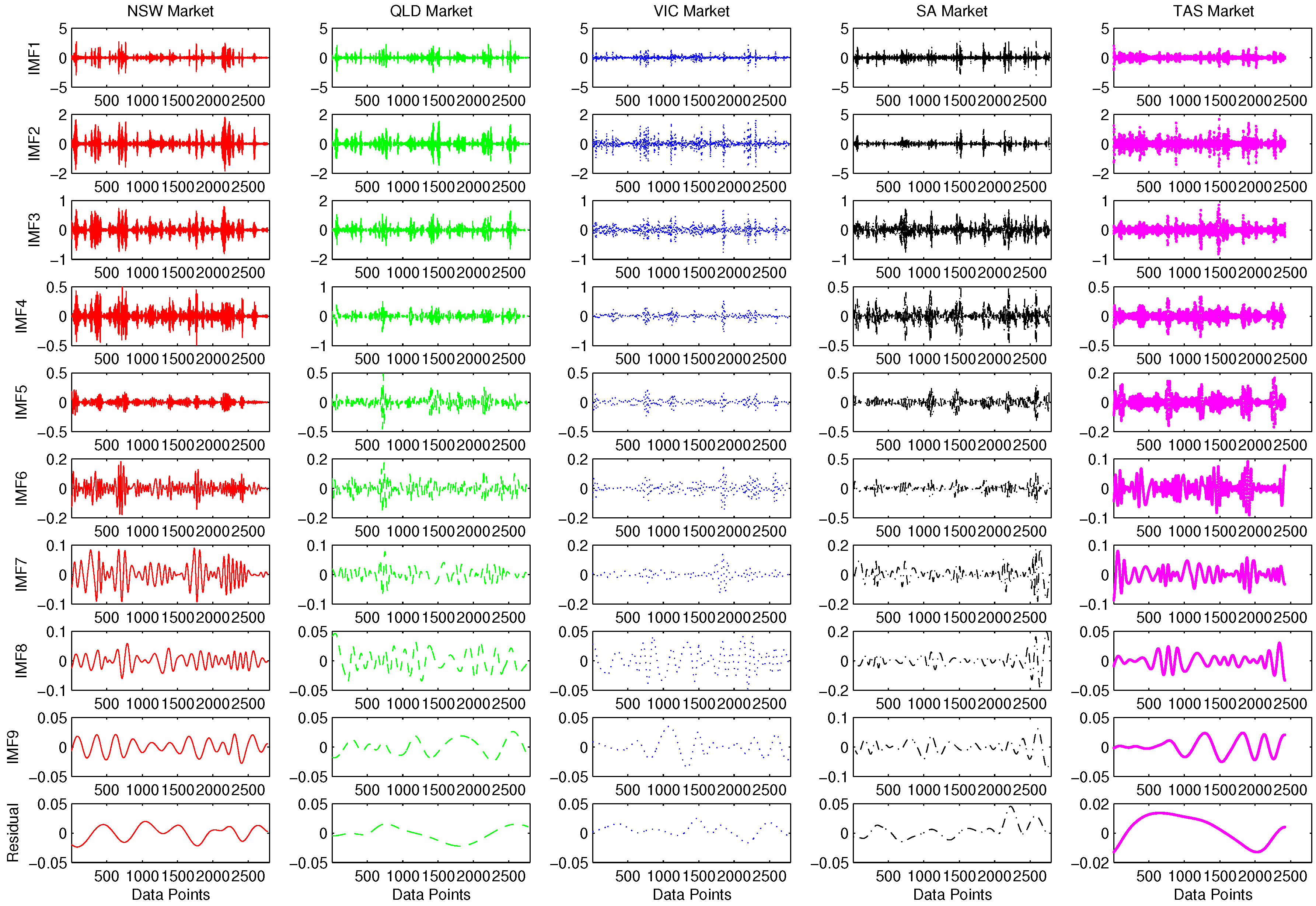
2.2. Empirical Mode Decomposition

Empirical Mode Decomposition (EMD) is a recent development in the signal processing field, besides the traditional Fourier and Wavelet analysis. Initially proposed for the physical disciplines such as biomedical engineering, structured health monitoring, image processing, etc., it has much potential and a wide range of applications in the economics and finance field as well [18,26]. Different from the Fourier analysis and wavelet analysis that use a fixed set of basis functions, the EMD model takes a data-driven non-parametric approach with the adaptive basis functions to decompose and analyze the time-varying data characteristics. This is particularly appealing when the model is applied to nonstationary and nonlinear data, where strict statistical data properties assumptions may not apply. The aim of the EMD model is to obtain the intrinsic mode functions (IMFs) as stable and stationary as possible. Thus, in practice, it offers more accurate representation of the data decomposition in the time scale domain, especially in the case of nonstationary data [13,27].

During the process when the empirical data are decomposed into different IMFs using Empirical Mode Decomposition (EMD), the following conditions are critical in defining the adaptively evolving basis, and serve as the stopping criteria for the optimization process for the model training.

• The number of extrema and zero-crossing should be the same, or differs at most by one;
• The functions are zero mean and symmetric, in terms of upper and lower envelope.

The algorithm for the EMD model is as follows:

• Given time series data $X\left(t\right)$, identify the locations for local maxima and minima of $X\left(t\right)$.
• Generate the upper envelope $u_{max}$ (lower envelope $u_{min}$) of the local maxima (minima) using local spline interpolation. Calculate the local mean $m\left(t\right)=(u_{max}+u_{min})/2$.
• Define the modulated oscillation $h\left(t\right)=X\left(t\right)-m\left(t\right)$ .
• If $h\left(t\right)$ satisfies (3), denote $h\left(t\right)$ as the ith IMF $c_i\left(t\right)$. Replace $X\left(t\right)$ with the residual $r\left(t\right)=X\left(t\right)-h\left(t\right)$. Otherwise, replace $X\left(t\right)$ with $h\left(t\right)$;

  $$\begin{array}{c}\hfill \mathrm{SD}=\sum _{t=0}^T\left[\frac{{\left|\left(h_{\left(k-1\right)}\left(t\right)-h_k\left(t\right)\right)\right|}^2}{h_{\left(k-1\right)}^2\left(t\right)}\right]\end{array}$$

  (3)
• Repeat the previous steps until the residual satisfies the stopping criteria. Then, the original electricity data is represented as two parts; i.e., the IMFs and the residue.

In Figure 1, using the sample return data in five Australian electricity markets, we provide a graphical illustration of the decomposed data structure and movements using the EMD model.

It can be seen from the illustration in Figure 1 that when the original data are projected into the multiscale domain, more micro-level data characteristics can be revealed. The frequency is monotonically decreasing with the increases in levels. For different IMFs across different scales, no markets seem to be more volatile than the others. The dominating forces for different markets are different at different scales.

2.3. Empirical Mode Decomposition (EMD)-Based Value at Risk Estimation

To apply the EMD model to the VaR estimation, we make two simplifying assumptions about the electricity market, as follows:

• Different investment strategies are stationary and mutually independent.
• Extreme or transient events would exhibit the biggest volatility.

The first assumption is consistent with the mainstream finance theory. For example, the normal demand is mainly long-term focused in their investment strategy. The peak demand is mainly short-term focused, looking for speculative opportunities. The behaviors of these two groups have lower levels of correlations.

As for the second assumption, we observe that extreme and transient events have significant and continuous influence on the electricity price fluctuation. The high level of fluctuation brought by these events has their unique frequency and scale characteristics.

With these two assumptions, the EMD-EWMA model is proposed, and consists of the following procedures:

Firstly, we use the EMD algorithm to decompose the in-sample return data into different IMFs.

Secondly, we take the simplified assumption that the IMF d with the biggest volatility is dominated with the extreme event. Thus, the IMF with the biggest volatility (i.e., standard deviation value in this paper) is identified and extracted. The remaining IMFs are identified as constituting the main factors behind the normal market behavior, suppressing the disruptive influence of the extreme events.

Thirdly, since IMFs are independent across different scales, the aggregated estimated volatility can be reconstructed from the summation of the estimated volatility of the retaining individual IMFs as in (4). We use the EWMA model to estimate the conditional standard deviation for the individual IMF.

$$\begin{array}{c}\hfill {\sigma }_{agg}\left(t\right)=\sqrt{\sum _{i=1}^{d-1}{\sigma }_{imf\left(i\right)}^2\left(t\right)+\sum _{i=d+1}^n{\sigma }_{imf\left(i\right)}^2\left(t\right)+{\sigma }_{Residual}^2\left(t\right)}\end{array}$$

(4)

where ${\sigma }_{agg}\left(t\right)$ is the aggregated volatility at time t. ${\sigma }_{imf\left(i\right)}\left(t\right)$ refers to the volatility of IMF at scale i at time t. ${\sigma }_{Residual}\left(t\right)$ refers to the volatility of the residual at time t.

Fourthly, the variance-covariance VaR model is used to forecast one day ahead VaR at time t, as in (5).

$$\begin{array}{c}\hfill VaR(\alpha ,t)=\left[\mu +{\sigma }_{agg}\left(t\right)Z_{\alpha ,w}\right]X\end{array}$$

(5)

where $Z_{\alpha ,w}$ refers to the quantile value, or the inverse Cumulative Density Function value, at the particular probability α of distribution w, w may refer to either normal distribution or Student’s t distribution. α takes the value of $1-cl$, $cl$ refers to the confidence level. In this paper we assume that the μ is zero.

Finally, we repeat steps 1–4 to make forecasts one step ahead.

3. Empirical Studies

In this paper, we use the extensive empirical data in the Australian electricity markets to conduct the experiments to evaluate the performance of the proposed model. The Australian electricity markets are chosen since it is one of the most deregulated markets in the world, representing some geographically diverse regions. The data sets are constructed using the daily observations from five sub-regions, including New South Wales (NSW), Queensland (QLD), South Australia (SA), Victoria (VIC), and Tasmania (TAS). The data is obtained from the website of the Australian National Energy Market (NEM). Except for NSW, negative and empty value are spotted in the other four markets due to potential recording errors. They are replaced with the smoothed values calculated using the interpolation method. The time period for the data set is from 1 January 2004 to 6 November 2014, except for the TAS market, which starts from 16 May 2005. The total number of observations is 3963, except for the TAS market, where the number of observations is 3462. The data set is divided based on a 70% ratio to be used for different purposes during the experiment. The daily price data have been transformed to scale free return data as in $y_t=ln\frac{p_t}{p_{t-1}}$. In this paper, VaR is estimated at daily frequency, and a one day holding period is assumed during VaR calculation.

To obtain the descriptive idea about the statistical characteristics of the data, we calculate the statistical moments and conduct the statistical tests. Four statistical moments include the mean, standard deviation, skewness, and kurtosis. The statistical tests include the Jarque-Bera test for normality and the Brock-Dechert-Scheinkman (BDS) test of independence [28,29,30].

Table 1. Descriptive statistics and statistical tests.

Markets	Mean	Standard Deviation	Skewness	Kurtosis	${\mathit{p}}_{\mathit{JB}}$	${\mathit{p}}_{\mathit{BDS}}$
$r_{NSW}$	0	0.3929	−0.4391	38.7708	0.001	0
$r_{QLD}$	0	0.4341	−0.1822	32.0143	0.001	0
$r_{SA}$	0	0.4824	0.4772	24.2047	0.001	0
$r_{TAS}$	0	0.3305	−0.5707	26.3124	0.001	0
$r_{VIC}$	0	0.3401	−0.1732	34.5017	0.001	0

Where mean, standard deviation, skewness, and kurtosis refer to the four moments describing the statistical distributions of the data. $p_{JB}$ and $p_{BDS}$ refer to the p value of the test statistics for Jarque-Bera (JB) test of normality and Brock-Dechert-Scheinkman (BDS) test of independence.

lists the descriptive statistics of returns for the five electricity markets.

From the results in Table 1, the electricity market returns deviate from the standard normal distribution, and there is significant risk exposure for investors in the market. There is significant standard deviation. The market returns lean towards loss on average, indicated by the negative skewness value. More importantly, we observe significantly large kurtosis value, deviating from the normal level, and indicating that the return changes significantly, partly because of an abnormal event. Besides, since both JB and BDS tests reject the null hypothesis, we can conclude that the market return distribution does not conform to a normal distribution and deviates from the independence.

In the meantime, different markets also exhibit their own unique characteristics. This is due to the limited physical transfer capability among different regions, as well as different degrees of market development from more deregulated NSWand QLD to the less deregulated SA market. Most notable is the positive skewness value for the SA market and the negative skewness value for other markets. The SA market had the highest level of standard deviation. This implies that among the five markets, the SA market is the most volatile and profitable, on average. This stylized fact is consistent with the unique characteristics of SA markets. The SA region is known for its very hot summer, with the peak electricity demand. The size of the market is relatively small, with limited coal and natural gas supply [31]. Thus, it behaves significantly differently from the other four markets. Meanwhile, the NSW market has the highest level of kurtosis. This implies that the degrees of extreme event influences vary among the five markets, where the impact of the extreme events is the most significant in NSW markets. It is the most deregulated and developed market, subject to external shocks and extreme events.

Then, we conducted empirical studies using the Australian electricity data set to evaluate the performance of the proposed model. To evaluate the model’s generalizability, we limit the models tested to EWMA model with elliptical distributions, including the normal and Student’s t distributions. Although different distributions exist in the literature, normal and Student’s t distributions are the most commonly used normal and non-normal distributions in the literature [32,33]. There have been research results reported on the use of non-normal distributions, such as skewed normal, skewed Student’s t distributions, etc. [34], but no consensus exists for their robustness and accuracy in capturing the empirical data distributions. In the meantime, the EWMA model is the most robust model, whose parameters optimization is less sensitive to the data set. Thus, the performance improvement with the proposed model can be attributed to the EMD model employed. The results and findings obtained can generalize to more complex risk measurement models such as the GARCH model with different underlying distributions. The performance improvements may vary, but are expected to be significant in different market circumstances.

In this paper, we use different kinds of forecasting measures to evaluate the model performance. These include the number of VaR exceedances, the p value for the Kupiec backtesting procedure, and the Mean Squared Error (MSE).The performance of different models under standard normal distribution are listed in

Table 2. Out-of-sample exceedances of different models under standard normal distribution.

Model	Market	${\mathit{Exc}}_{95\%}$	${\mathit{Exc}}_{97.5\%}$	${\mathit{Exc}}_{99\%}$	$\overline{\mathit{Exc}}$	${\mathit{P}}_{95\%}$	${\mathit{P}}_{97.5\%}$	${\mathit{P}}_{99\%}$	$\overline{\mathit{P}}$	${\mathit{MSE}}_{95\%}$	${\mathit{MSE}}_{97.5\%}$	${\mathit{MSE}}_{99\%}$	$\overline{\mathit{MSE}}$
	SA	28	14	8	16.6667	0	0.0011	0.227	0.0760	52.9937	59.4396	67.9623	60.1319
	TAS	33	20	12	21.6667	0.0039	0.2145	0.6264	0.2816	17.7443	20.0184	22.8756	20.2128
EWMA	VIC	33	16	9	19.3333	0.0001	0.0052	0.3773	0.1275	31.9751	34.9794	39.329	35.4278
	NSW	34	22	10	22.0000	0.0002	0.1316	0.5692	0.2337	13.6768	15.0194	16.8504	15.1822
	QLD	31	18	10	19.6667	0	0.0187	0.5692	0.1960	41.4191	47.1902	54.4574	47.6889
	SA	65	42	25	44.0000	0.4707	0.032	0.0009	0.1679	46.3525	49.41	53.8644	49.8756
	TAS	54	45	32	43.6667	0.7773	0.0006	0	0.2593	15.8873	17.4368	19.4366	17.5869
EMD-EWMA	VIC	79	42	21	47.3333	0.0133	0.032	0.0167	0.0207	32.5269	34.2162	36.7786	34.5072
	NSW	74	49	32	51.6667	0.0627	0.0011	0	0.0213	14.354	15.652	17.3934	15.7998
	QLD	58	39	24	40.3333	0.8412	0.1009	0.0019	0.3147	38.9737	43.9293	50.2608	44.3879

.

From results in Table 2, it can be seen that the exceedances of the proposed EMD-EWMA model under all the confidence levels are higher than that of the EWMA model. As far as p value is concerned, our proposed model achieved mixed performance under different confidence levels against the benchmark EWMA. It performs better at the $95\%$ confidence level, but it performs worse at the $99\%$ confidence level. Overall, the EMD-EWMA model does not show significant improvement in risk coverage. Results in Table 2 show that MSEs of the proposed EMD-EWMA model are lower than that of the EWMA model under all three confidence levels($95\%$, $97.5\%$, $99\%$). The predictive accuracy of the proposed EMD-EWMA model largely improves upon the traditional EWMA model.

To further improve the model performance, we noted that electricity market return distribution may not satisfy the normal distribution during the VaR estimation. Since the electricity market returns do not conform to standard normal distribution, we use the Student’s t distribution to estimate VaR and conduct the empirical studies, and we use $T_{\alpha }$ representing Student’s t distribution instead of $Z_{\alpha }$. The corresponding exceedances, p values, and MSEs are listed in

Table 3. Out-of-sample exceedances of different models under Student’s t distribution.

Model	Market	${\mathit{Exc}}_{95\%}$	${\mathit{Exc}}_{97.5\%}$	${\mathit{Exc}}_{99\%}$	$\overline{\mathit{Exc}}$	${\mathit{P}}_{95\%}$	${\mathit{P}}_{97.5\%}$	${\mathit{P}}_{99\%}$	$\overline{\mathit{P}}$	${\mathit{MSE}}_{95\%}$	${\mathit{MSE}}_{97.5\%}$	${\mathit{MSE}}_{99\%}$	$\overline{\mathit{MSE}}$
	SA	22	8	2	10.6667	0	0	0.0004	0.0001	56.3005	65.591	79.1048	66.9988
	TAS	26	14	4	14.6667	0	0.0091	0.0226	0.0106	18.9285	22.0918	26.4875	22.5026
EWMA	VIC	20	13	2	11.6667	0	0.0005	0.0004	0.0003	33.4747	38.0882	45.37	38.9776
	NSW	29	12	5	15.3333	0	0.0002	0.023	0.0077	14.3598	16.336	19.3053	16.6670
	QLD	23	11	6	13.3333	0	0.0001	0.0574	0.0192	44.4216	52.4633	63.643	53.5093
	SA	46	27	12	28.3333	0.0619	0.6041	0.9768	0.5476	48.0837	53.0234	61.0517	54.0529
	TAS	49	36	21	35.3333	0.6666	0.0603	0.0037	0.2435	16.7912	19.0735	22.3791	19.4146
EMD-EWMA	VIC	59	24	13	32.0000	0.9469	0.2695	0.7522	0.6562	33.4739	36.2884	41.0526	36.9383
	NSW	61	36	20	39.0000	0.8425	0.261	0.0315	0.3783	15.1041	17.0733	20.0307	17.4027
	QLD	46	27	12	28.3333	0.0619	0.6041	0.9768	0.5476	41.8694	49.1166	59.4536	50.1465

.

Results in Table 3 show that the performance of the proposed EMD-EWMA model using the Student’s t distribution improve significantly upon the benchmark models, in terms of both risk coverage and predictive accuracy.

Firstly, the exceedances of EMD-EWMA model using Student’s t distribution are higher than that of EWMA using Student’s t distribution. Secondly, traditional EWMA model tends to overestimate VaR, shown by the relatively lower Kupiec p values. On the contrary, most p values of the EMD-EWMA model are over 0.05, which shows great risk coverage. Moreover, except in TAS and NSW under the $99\%$ confidence level, all the other p values of the EMD-EWMA model are higher than that of EWMA. Thirdly, as for MSE, the EMD-EWMA model demonstrates the improved predictive accuracy by a large margin compared to the EWMA model. For SA, TAS, VIC, and QLD markets, the MSEs of the EMD-EWMA model are lower than that of the EWMA model. For the NSW market, the MSE is only slightly higher than that of the EWMA model. The proposed model performs competently in terms of predictive accuracy in the NSW market.

More importantly, the utilized EWMA model in the proposed EMD-EWMA model is widely recognized as the most robust and stable model, due to its simple form. It is nested within the proposed EMD-EWMA model. Thus, the performance improvement of the proposed model can be attributed to the introduction of the EMD model to analyze and model the additional data features refreshed in the multiscale data domain.

4. Conclusions

In this paper, we have proposed a new EMD-EWMA-based model to estimate VaR. Experiments using Australian electricity market data show that the introduced EMD model can be used to analyze and separate the underlying data components of distinct characteristics. We separate and remove the the data components influenced by the extreme and transient event, thus improving the model fit for the remaining data components. The incorporation of the EMD model in the traditional EWMA model has resulted in a significant performance improvement. We also find that switching from the normal distribution to Student’s t distribution improves the model performance.

Work in this paper has some further implications. Since the adopted EWMA model is simple and robust, and is nested with the proposed model, the performance improvement is attributed to the EMD model introduced. The statistically significantly higher reliability and accuracy achieved suggests that the multiscale-based methodology better characterizes the heterogeneous market structure with the improved forecasting performance. This shows that a diverse range of heterogeneous risk data features exist in the market and need to be incorporated in the model. Besides, different risk factors in the multiscale domain need to be identified and modeled. Depending on the risk preference and investment strategies adopted, model specifications and parameters for different risk factors across time scales can vary considerably.

References

1. Deng, S.; Oren, S. Electricity derivatives and risk management. Energy 2006, 31, 940–953. [Google Scholar] [CrossRef]
2. Liu, M.; Wu, F.F. Risk management in a competitive electricity market. Int. J. Electr. Power Energy Syst. 2007, 29, 690–697. [Google Scholar] [CrossRef]
3. Pineda, S.; Conejo, A.J. Managing the financial risks of electricity producers using options. Energy Econ. 2012, 34, 2216–2227. [Google Scholar] [CrossRef]
4. Shenoy, S.; Gorinevsky, D. Data-driven stochastic pricing and application to electricity market. IEEE J. Sel. Top. Signal Proces. 2016, 10, 1029–1039. [Google Scholar] [CrossRef]
5. Kaye, R.; Outhred, H.; Bannister, C.H. Forward contracts for the operation of an electricity industry under spot pricing. IEEE Trans. Power Syst. 1990, 5, 46–52. [Google Scholar] [CrossRef]
6. Tanlapco, E.; Lawarree, J.; Liu, C.C. Hedging with futures contracts in a deregulated electricity industry. IEEE Trans. Power Syst. 2002, 17, 577–582. [Google Scholar] [CrossRef]
7. Dahlgren, R.; Liu, C.C.; Lawarree, J. Risk assessment in energy trading. IEEE Trans. Power Syst. 2003, 18, 503–511. [Google Scholar] [CrossRef]
8. Walls, W.; Zhang, W. Using extreme value theory to model electricity price risk with an application to the alberta power market. Energy Explor. Exploit. 2005, 23, 375–403. [Google Scholar] [CrossRef]
9. Chan, F.; Gray, P. Using extreme value theory to measure value-at-risk for daily electricity spot prices. Int. J. Forecast. 2006, 22, 283–300. [Google Scholar] [CrossRef]
10. Peters, E.E. Chaos and Order in the Capital Markets: A New View of Cycles, Prices, and Market Volatility; John Wiley & Sons: New York, NY, USA, 1996; Volume 1. [Google Scholar]
11. Lux, T.; Marchesi, M. Scaling and criticality in a stochastic multi-agent model of a financial market. Nature 1999, 397, 498–500. [Google Scholar] [CrossRef]
12. Karandikar, R.G.; Deshpande, N.R.; Khaparde, S.A.; Kulkarni, S.V. Modelling volatility clustering in electricity price return series for forecasting value at risk. Eur. Trans. Electr. Power 2009, 19, 15–38. [Google Scholar] [CrossRef]
13. Huang, N.E.; Wu, M.L.; Qu, W.; Long, S.R.; Shen, S.S. Applications of Hilbert–Huang transform to non-stationary financial time series analysis. Appl. Stoch. Model. Bus. Ind. 2003, 19, 245–268. [Google Scholar] [CrossRef]
14. Yu, L.; Wang, S.; Lai, K.K. Forecasting crude oil price with an EMD-based neural network ensemble learning paradigm. Energy Econ. 2008, 30, 2623–2635. [Google Scholar] [CrossRef]
15. Premanode, B.; Toumazou, C. Improving prediction of exchange rates using differential EMD. Expert Syst. Appl. 2012, 40, 377–384. [Google Scholar] [CrossRef]
16. Premanode, B.; Vonprasert, J.; Toumazou, C. Prediction of exchange rates using averaging intrinsic mode function and multiclass support vector regression. Artif. Intell. Res. 2013, 2, 47. [Google Scholar] [CrossRef]
17. Wu, M.C. Phase correlation of foreign exchange time series. Phys. A Stat. Mech. Appl. 2007, 375, 633–642. [Google Scholar] [CrossRef]
18. Zhang, X.; Lai, K.; Wang, S.Y. A new approach for crude oil price analysis based on Empirical Mode Decomposition. Energy Econ. 2008, 30, 905–918. [Google Scholar] [CrossRef]
19. An, N.; Zhao, W.; Wang, J.; Shang, D.; Zhao, E. Using multi-output feedforward neural network with empirical mode decomposition based signal filtering for electricity demand forecasting. Energy 2012, 49, 279–288. [Google Scholar] [CrossRef]
20. Dong, Y.; Wang, J.; Jiang, H.; Wu, J. Short-term electricity price forecast based on the improved hybrid model. Energy Convers. Manag. 2011, 52, 2987–2995. [Google Scholar] [CrossRef]
21. Dowd, K. Measuring Market Risk, 2nd ed.; John Wiley & Sons: West Sussex, UK, 2005. [Google Scholar]
22. He, K.; Lai, K.K.; Xiang, G. Portfolio value at risk estimate for crude oil markets: A multivariate wavelet denoising approach. Energies 2012, 5, 1018–1043. [Google Scholar] [CrossRef]
23. He, K.; Xie, C.; Chen, S.; Lai, K.K. Estimating VaR in crude oil market: A novel multi-scale non-linear ensemble approach incorporating wavelet analysis and neural network. Neurocomputing 2009, 72, 3428–3438. [Google Scholar] [CrossRef]
24. He, K.; Lai, K.K.; Yen, J. Ensemble forecasting of value at risk via multi resolution analysis based methodology in metals markets. Expert Syst. Appl. 2012, 39, 4258–4267. [Google Scholar] [CrossRef]
25. He, K.; Lai, K.K.; Yen, J. Value-at-risk estimation of crude oil price using MCA based transient risk modeling approach. Energy Econ. 2011, 33, 903–911. [Google Scholar] [CrossRef]
26. Xu, G.; Wang, X.; Xu, X.; Zhou, L. Improved EMD for the analysis of FM signals. Mech. Syst. Signal Process. 2012, 33, 181–196. [Google Scholar]
27. Yu, L.; Wang, S.; Lai, K.K. Credit risk assessment with a multistage neural network ensemble learning approach. Expert Syst. Appl. 2008, 34, 1434–1444. [Google Scholar] [CrossRef]
28. Brooks, C. Introductory Econometrics for Finance, 2nd ed.; Cambridge University Press: Cambridge, UK, 2008. [Google Scholar]
29. Brock, W.A.; Hsieh, D.A.; LeBaron, B.D. Nonlinear Dynamics, Chaos, and Instability: Statistical Theory and Economic Evidence; MIT Press: Cambridge, MA, USA, 1991. [Google Scholar]
30. Panagiotidis, T. Testing the assumption of linearity. Econ. Bull. 2002, 3, 1–9. [Google Scholar]
31. Spoehr, J. Power Politics: The Electricity Crisis and You; Wakefield Press: Kent Town, Australia, 2003. [Google Scholar]
32. Lien, D.; Yang, X.B.; Ye, K.Y. Alternative approximations to value-at-risk: A comparison. Commun. Stat. Simul. Comput. 2014, 43, 2225–2240. [Google Scholar] [CrossRef]
33. Andriosopoulos, K.; Nomikos, N. Risk management in the energy markets and Value-at-Risk modelling: A hybrid approach. Eur. J. Financ. 2015, 21, 548–574. [Google Scholar] [CrossRef]
34. Gencer, H.G.; Demiralay, S. Volatility modeling and value-at-risk (var) forecasting of emerging stock markets in the presence of long memory, asymmetry, and skewed heavy tails. Emerg. Mark. Financ. Trade 2016, 52, 639–657. [Google Scholar] [CrossRef]
Figure 1. Decomposed Intrinsic Mode Functions (IMFs) using the Empirical Mode Decomposition (EMD) algorithm in Australian electricity markets. NSW: New South Wales; QLD: Queensland; SA: South Australia; VIC: Victoria; TAS: Tasmania.
Energies 09 00931 g001