
The Economic Viability of Renewable Portfolio Standard Support for Offshore Wind Farm Projects in Korea


Abstract
:1. Introduction
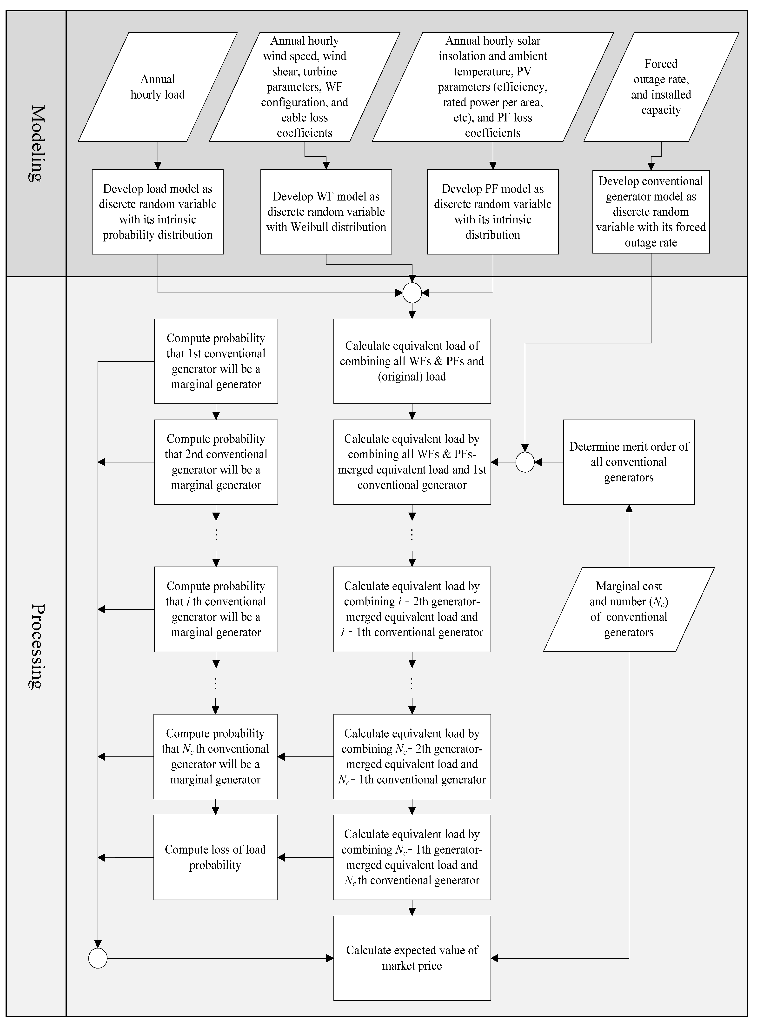
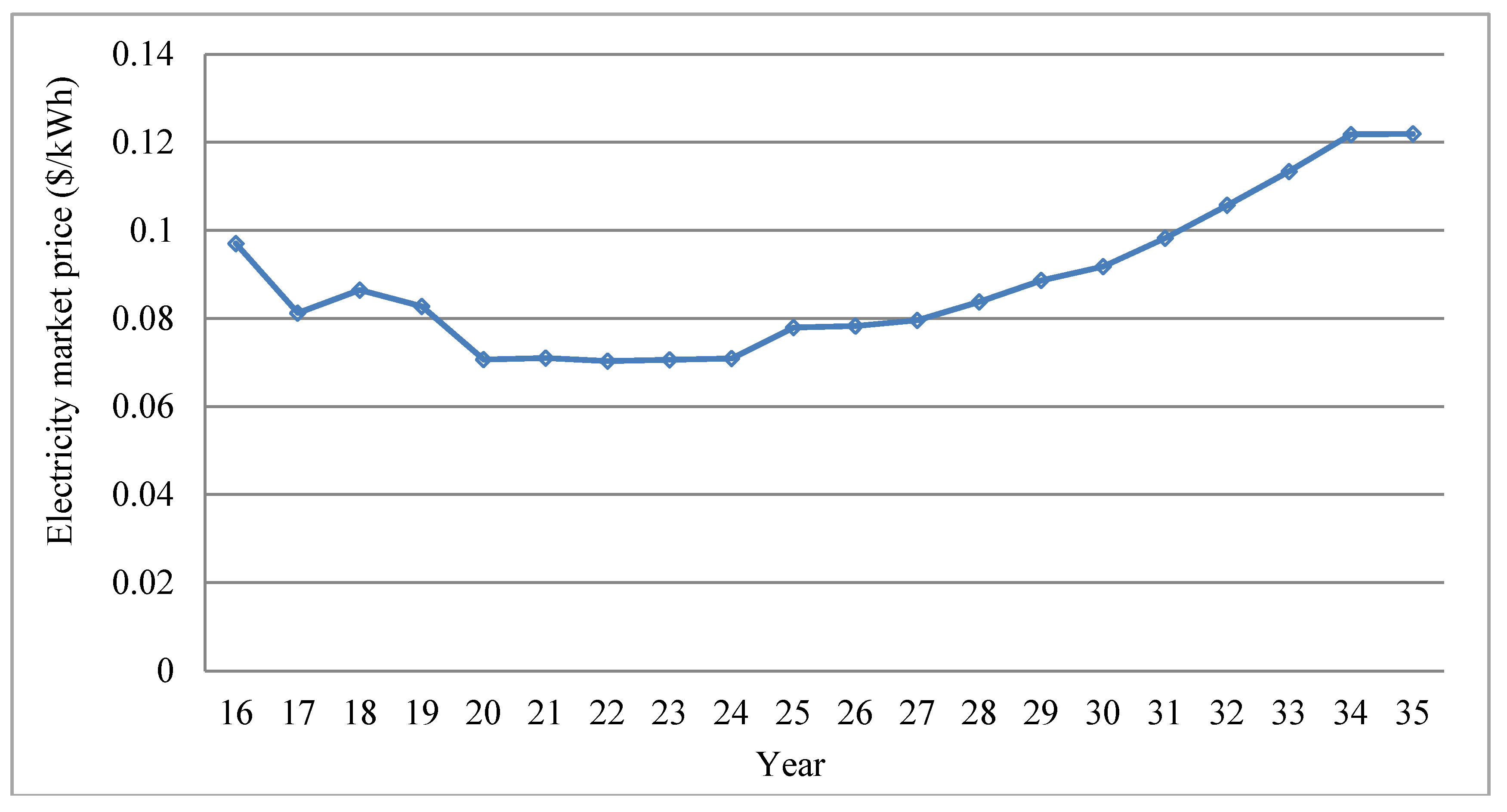
2. Predicting the Market Price of Electricity

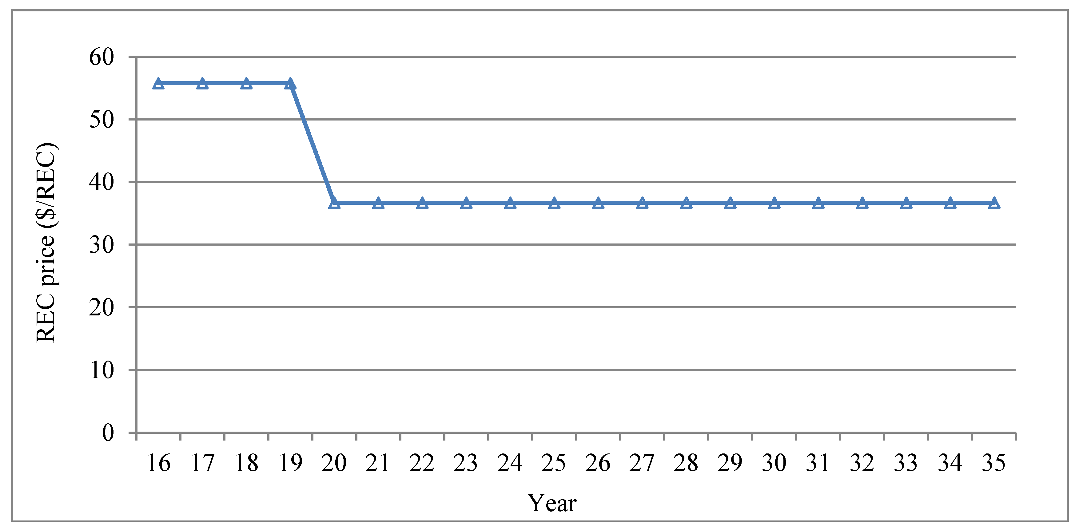
3. Predicting the REC (Renewable Energy Certificate) Price

| Year | 2015 | 2016 | 2017 | 2018 | 2019 | 2020 | 2021 | After 2021 |
|---|---|---|---|---|---|---|---|---|
| Fraction of renewable energy | 3.5% | 4% | 5% | 6% | 7% | 8% | 9% | 10% |
4. Assessment of Wind Energy Production
5. Revenue and Cost for Offshore Wind Farms
6. Metrics of Economic Evaluation
7. Case Study

| Fuel Type | Capacity (MW) | |
|---|---|---|
| Nuclear | 24,516 | |
| Coal | 28,294 | |
| Gas | 31,372 | |
| Oil | 3161 | |
| Renewable energy | Wind | 3286 |
| Solar | 1807 | |
| Other | 3610 | |
| Other sources | 11,073 | |
| Total installed capacity | 107,119 | |
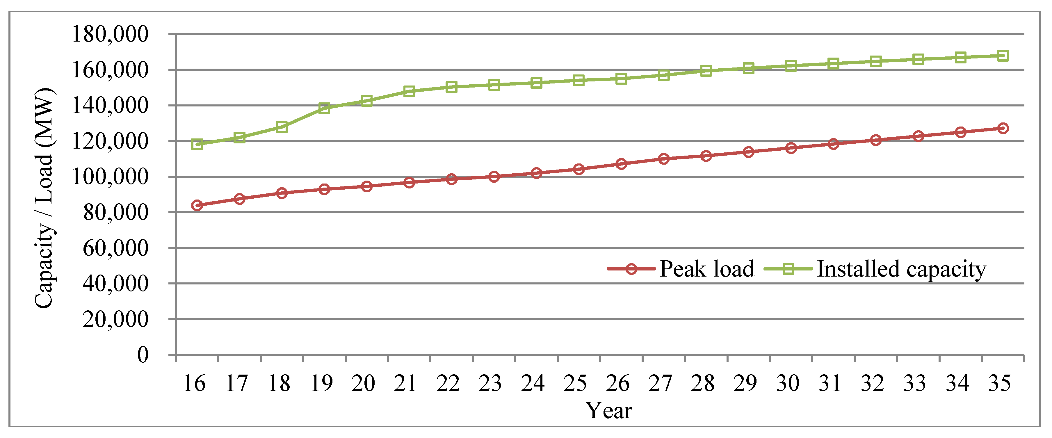
| Year | Nuclear (MW) | Coal (MW) | Gas (MW) | Oil (MW) | Renewable Energy | Other Sources (MW) | Total Installed Capacity (MW) | ||
|---|---|---|---|---|---|---|---|---|---|
| Wind (MW) | Solar (MW) | Other (MW) | |||||||
| 2016 | 0 | 7760 | 1752 | −809 | 1070 | 1 | 109 | 1127 | 118,129 |
| 2017 | 1400 | 600 | 950 | 812 | 485 | 4 | 334 | −810 | 121,904 |
| 2018 | 1400 | 2370 | −480 | 0 | 2430 | 0 | 200 | 1 | 127,825 |
| 2019 | 1400 | 5370 | 0 | 0 | 2246 | 32 | 743 | 744 | 138,360 |
| 2020 | 1400 | 0 | 0 | 0 | 1506 | 9 | 1256 | 3 | 142,534 |
| 2021 | 1400 | 1000 | 0 | 0 | 2700 | 0 | 206 | −3 | 147,837 |
| 2022 | 1400 | 0 | 0 | 0 | 1880 | 70 | 289 | −1200 | 150,276 |
| 2023 | 1500 | 0 | −1800 | −1200 | 450 | 795 | 238 | 1200 | 151,459 |
| 2024 | 1500 | 0 | 0 | 0 | 0 | 840 | 240 | −1400 | 152,639 |
| 2025 | 0 | 0 | 0 | 0 | 0 | 863 | 541 | 0 | 154,043 |
| 2026 | 0 | 0 | 0 | −1400 | 0 | 0 | 876 | 1400 | 154,919 |
| 2027 | 0 | 0 | 0 | 0 | 1222 | 993 | −255 | 0 | 156,879 |
| 2028 | 0 | 0 | 0 | 0 | 715 | 565 | 272 | 922 | 159,353 |
| 2029 | 0 | 0 | 0 | 0 | 699 | 521 | 284 | −50 | 160,806 |
| 2030 | 0 | 0 | 0 | 0 | 681 | 476 | 299 | −96 | 162,166 |
| 2031 | 0 | 0 | 0 | 0 | 661 | 432 | 315 | −130 | 163,443 |
| 2032 | 0 | 0 | 0 | 0 | 639 | 387 | 333 | −155 | 164,647 |
| 2033 | 0 | 0 | 0 | 0 | 615 | 343 | 353 | −172 | 165,786 |
| 2034 | 0 | 0 | 0 | 0 | 591 | 299 | 374 | −182 | 166,867 |
| 2035 | 0 | 0 | 0 | 0 | 565 | 254 | 396 | −187 | 167,895 |
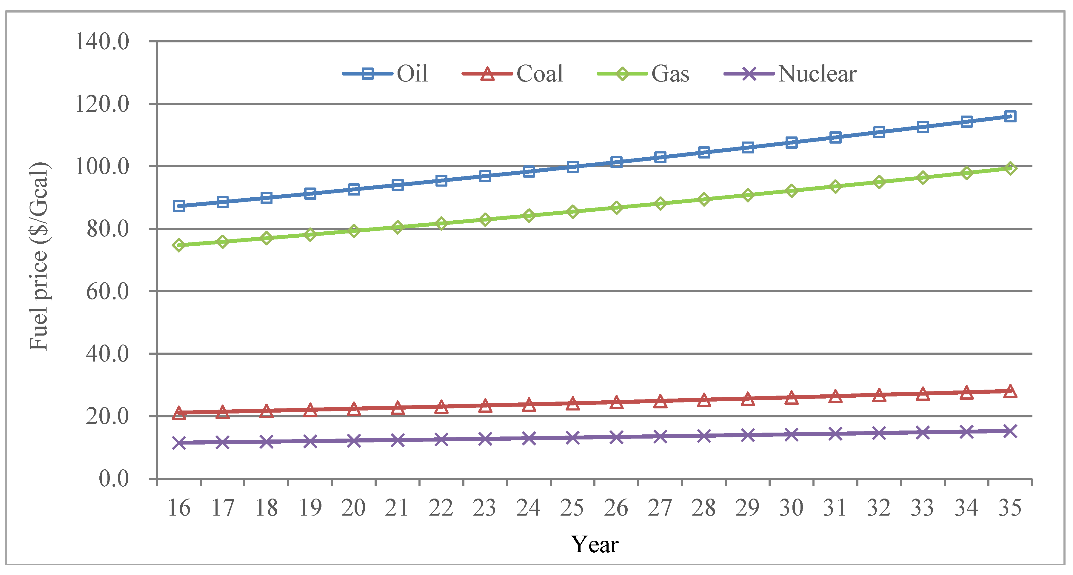
| Fuel Type | Marginal Cost ($/kWh) | FOR |
|---|---|---|
| Coal | 0.0289 | 0.048 |
| Gas | 0.1522 | 0.07 |
| Oil | 0.1160 | 0.05 |
| Other | 0.0058 | 0.015 |


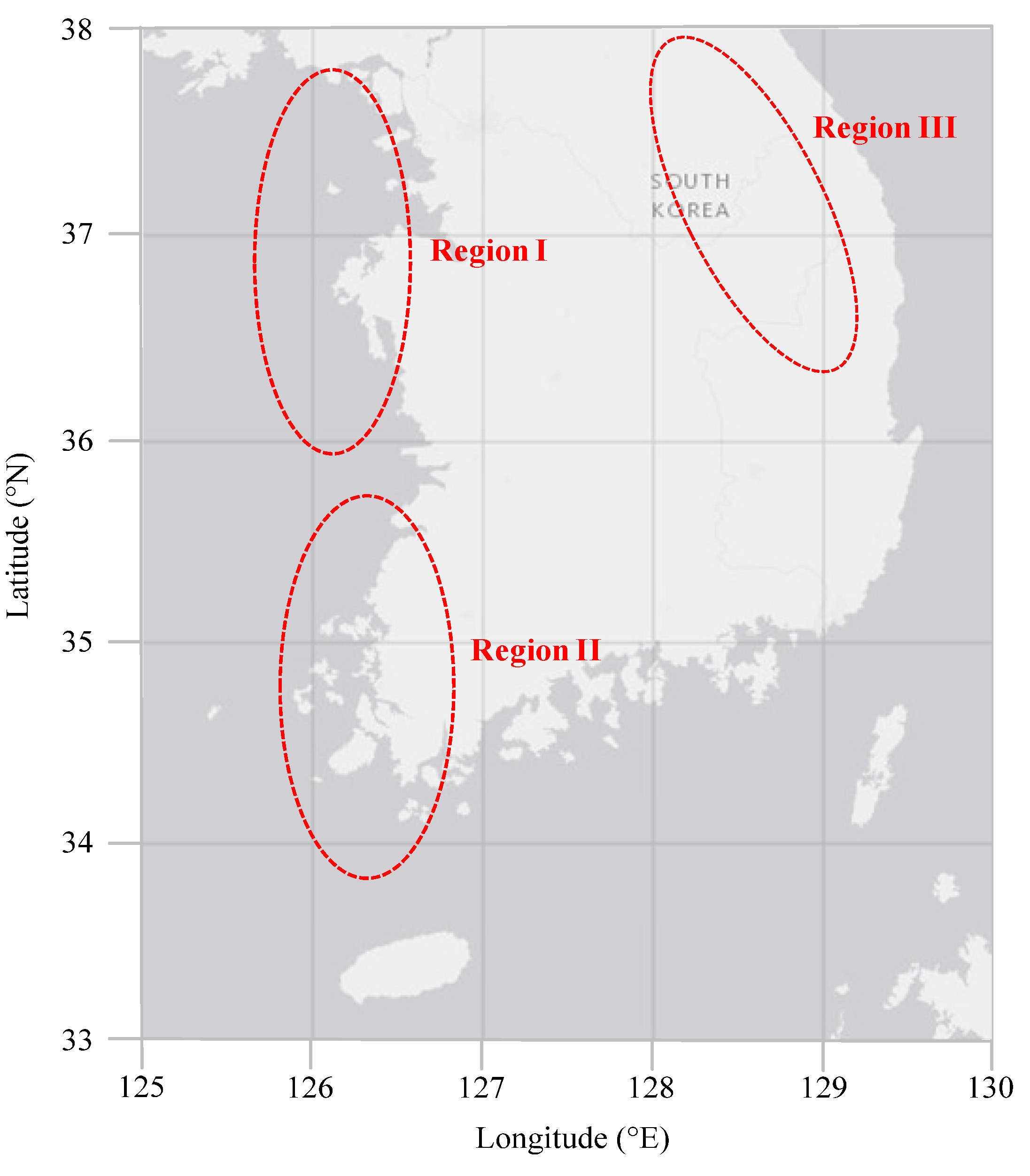
| Region | Average Wind Speed (m/s) | Shape Parameter | Capacity Factor |
|---|---|---|---|
| I | 5.925 | 1.8887 | 24.3% |
| II | 6.300 | 1.8091 | 27.8% |
| III | 7.073 | 1.3526 | 30.8% |
| Term | Description |
|---|---|
| Wind turbine | |
| Model | NREL 5-MW Baseline WT |
| Rated power (MW) | 5 |
| Cut-in wind speed (m/s) | 3 |
| Rated wind speed (m/s) | 11.4 |
| Cut-off wind speed (m/s) | 25 |
| Rotor diameter (m) | 127.5 |
| Hub height (m) | 90 |
| Maximum CP | 0.466 |
| Conversion loss coefficients | Quadratic = 0, Linear = 0.055, Constant = 0.02 |
| Monopile-type foundation | |
| Steel cost ($/kg) | 0.751 |
| Steel density (kg/m3) | 7870 |
| Monopile diameter (m) | 5.5695 |
| Monopile thickness (m) | 0.075 |
| Wind farm | |
| Size | 100 MW |
| Configuration | 2 WTs × 10 WTs |
| Spacing between WTs | 10 diameters ×10 diameters |
| Others | |
| Wind shear exponent | 0.143 |
| Air density (kg/m3) | 1.228 |
| Submarine cable loss coefficient | Internal = 0.025, External = 0.04 |
| Availability | 0.98 |
| Item | Figure |
|---|---|
| Inflation rate | 3% |
| Nominal discount rate | 7.12% |
| Corporate tax rate | 22% |
| Loan fraction | 65% |
| Loan interest rate | 4% |
| Amortization period (years) | 10 |
| Grace period (years) | 3 |
| Depreciation period (years) | 15 |
| Construction period (years) | 3 |
| Operations period (years) | 20 |

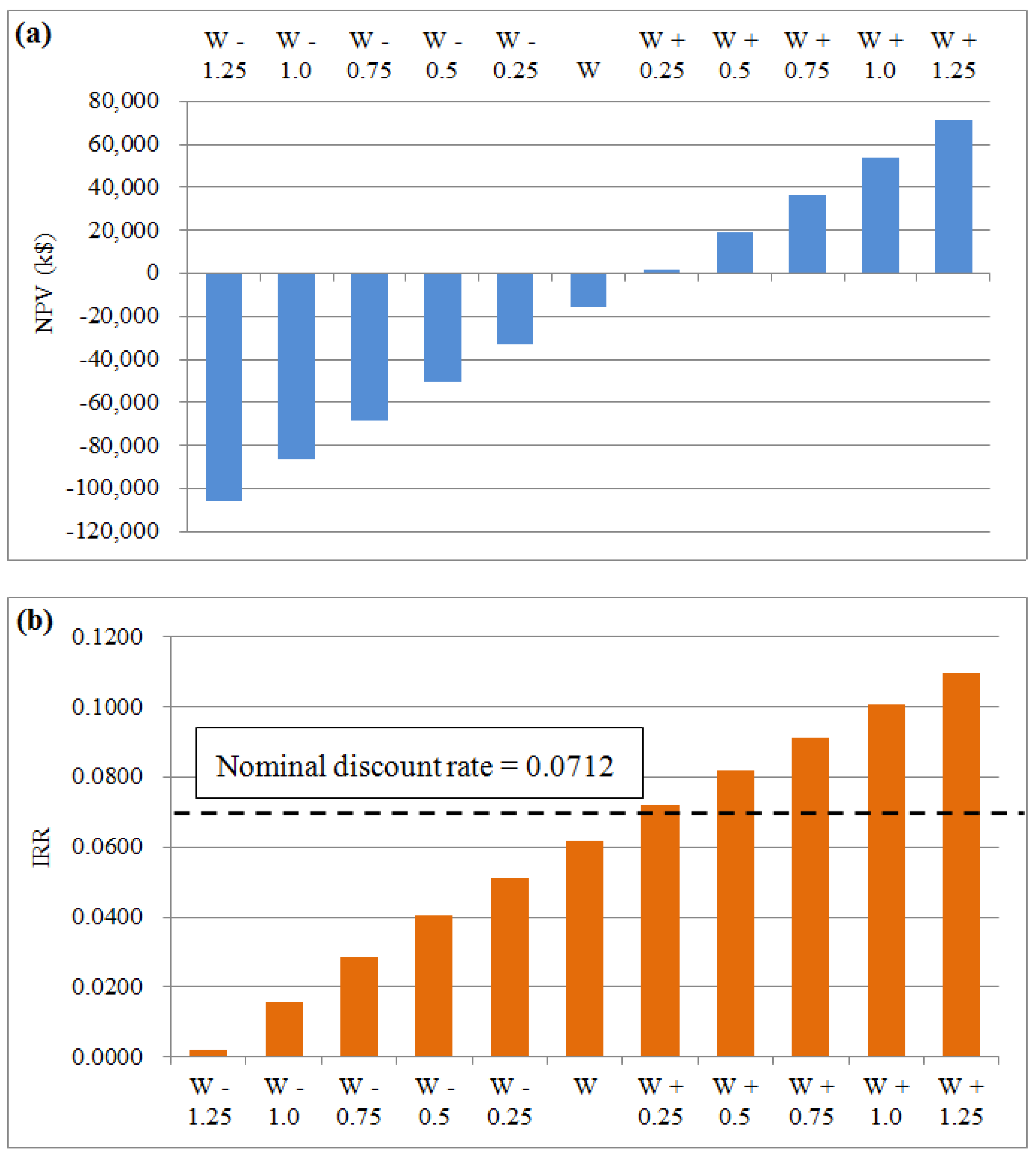
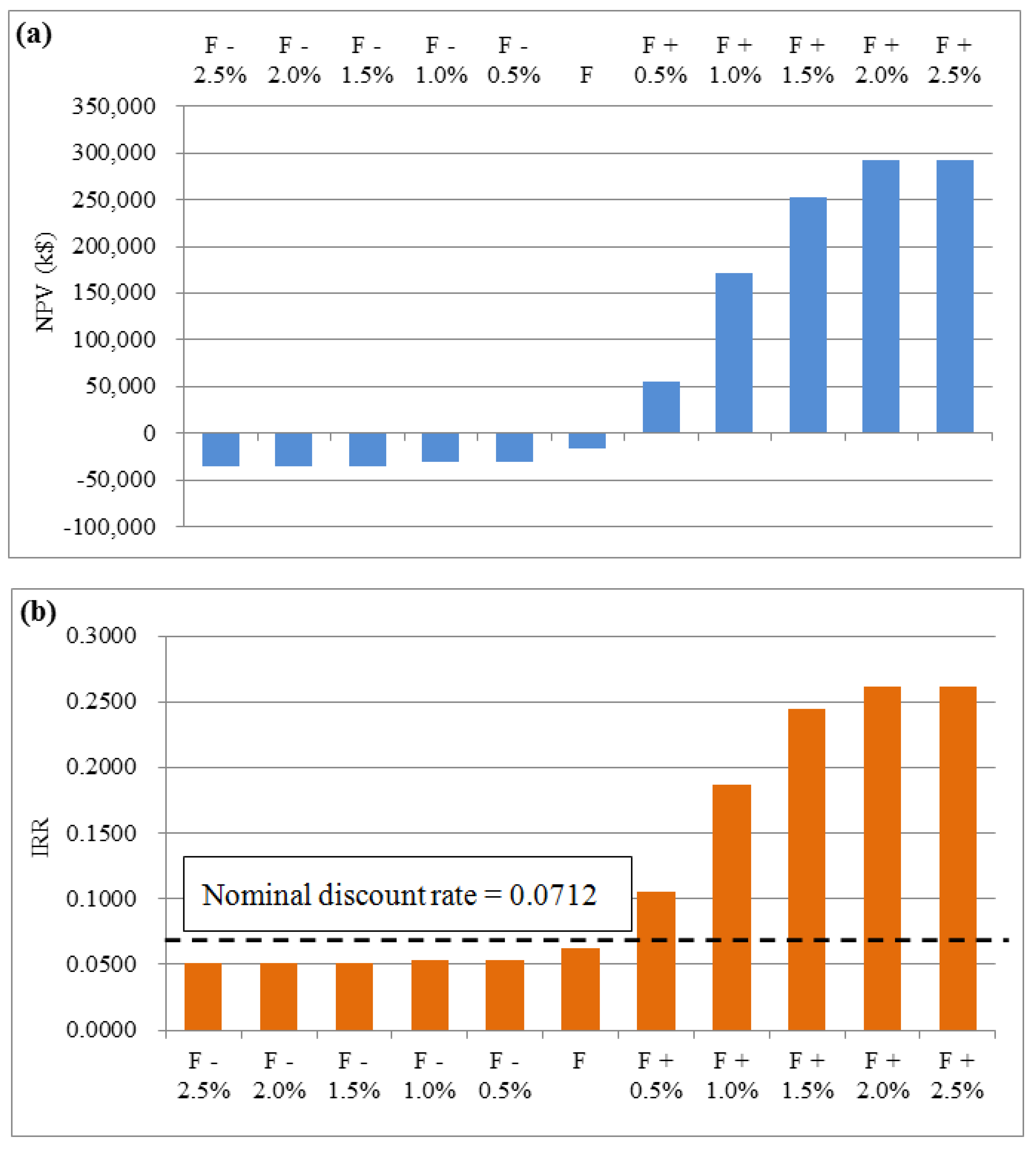
| Scenario 1: Adjustment for REC Weighting | Scenario 2: Adjustment for MMF |
|---|---|
| W − 1.25 | F − 2.5% |
| W − 1.0 | F − 2.0% |
| W − 0.75 | F − 1.5% |
| W − 0.5 | F − 1.0% |
| W − 0.25 | F − 0.5% |
| W | F |
| W + 0.25 | F + 0.5% |
| W + 0.5 | F + 1.0% |
| W + 0.75 | F + 1.5% |
| W + 1.0 | F + 2.0% |
| W + 1.25 | F + 2.5% |
8. Conclusions
Acknowledgments
Author Contributions
Conflicts of Interest
Nomenclature
| AWEP | Annual wind energy production |
| AWEPWF | AWEP of a WF |
| AWEPWT | AWEP of a WT |
| Ci | Cumulative sum of installed capacities of all conventional generators up to the ith conventional generator |
| dL | Infinitesimal increment in load |
| EPP | Electric power producer |
| fC,i | PDF of unavailable capacity of ith conventional generator |
| fi | PDF of equivalent load of ith conventional generator |
| FIT | Feed-in tariff |
| fL | PDF of original load |
| FOR | Forced outage rate |
| FORi | FOR of ith conventional generator |
| fP,# | PDF of output of PF # multiplied by −1 |
| fW,# | PDF of output of WF # multiplied by −1 |
| fWP | PDF of equivalent load incorporating M WFs and N PFs |
| I | Index of conventional generator |
| IRR | Internal rate of return |
| K | Index for type of renewable energy resource |
| LCOE | Levelized cost of energy |
| M | Number of WFs |
| MMF | Mandatory minimum fraction |
| N | Number of PFs |
| Nc | Number of conventional generators |
| NPV | Net present value |
Probability density function | |
| PF | PV farm |
| PPC | Probabilistic production cost |
| PV | Photovoltaic |
| REC | Renewable energy certificate |
| RPS | Renewable portfolio standard |
| T | Year of operation of WF |
| WF | Wind farm |
| WT | Wind turbine |
References
- The Ministry of Knowledge Economy. The 6th Basic Plan on Electricity Demand and Supply; The Ministry of Knowledge Economy: Sejong City, Korea, 2013. [Google Scholar]
- Yu, J.-H. Special issues on wind-roadmap for promoting offshore wind power. J. Electr. World 2010, 408, 56–59. [Google Scholar]
- Lee, S.-M.; Han, H.-S. Benefit-cost analysis of biodiesel production in Korea. J. Rural Dev. 2008, 31, 49–65. [Google Scholar]
- Chen, W.-M.; Kim, H.; Yamaguchi, H. Renewable energy in Eastern Asia: Renewable energy policy review and comparative SWOT analysis for promoting renewable energy in Japan, South Korea, and Taiwan. Energy Policy 2014, 74, 319–329. [Google Scholar] [CrossRef]
- Hwang, S.; Kwon, J.; Ahn, J.; Woo, P.-S.; Kim, B.H. A study on the rec price for the RPS. In Proceedings of the 43th the KIEE Summer Annual Conference, Gangwon-do, Korea, 18–20 July 2012; pp. 352–354.
- Korea Power Exchange (KPX). Annual Market Operation Data; KPX: Seoul, Korea, 2013. [Google Scholar]
- Cutler, N.J.; Boerema, N.D.; MacGill, I.F.; Outhred, H.R. High penetration wind generation impacts on spot prices in the australian national electricity market. Energy Policy 2011, 39, 5939–5949. [Google Scholar] [CrossRef]
- Morales, J.M.; Conejo, A.J.; Perez-Ruiz, J. Simulating the impact of wind production on locational marginal prices. IEEE Trans. Power Syst. 2011, 26, 820–828. [Google Scholar] [CrossRef]
- Rahimiyan, M. A statistical cognitive model to assess impact of spatially correlated wind production on market behaviors. Appl. Energy 2014, 122, 62–72. [Google Scholar] [CrossRef]
- Vilim, M.; Botterud, A. Wind power bidding in electricity markets with high wind penetration. Appl. Energy 2014, 118, 141–155. [Google Scholar] [CrossRef]
- Pereira, A.J.; Saraiva, J.T. Long term impact of wind power generation in the Iberian day-ahead electricity market price. Energy 2013, 55, 1159–1171. [Google Scholar] [CrossRef]
- Rubin, O.D.; Babcock, B.A. The impact of expansion of wind power capacity and pricing methods on the efficiency of deregulated electricity markets. Energy 2013, 59, 676–688. [Google Scholar] [CrossRef]
- Lind, A.; Rosenberg, E.; Seljom, P.; Espegren, K.; Fidje, A.; Lindberg, K. Analysis of the EU renewable energy directive by a techno-economic optimisation model. Energy Policy 2013, 60, 364–377. [Google Scholar] [CrossRef]
- Sawhney, R.; Thakur, K.; Venkatesan, B.; Ji, S.; Upreti, G.; Sanseverino, J. Empirical analysis of the solar incentive policy for Tennessee solar value chain. Appl. Energy 2014, 131, 368–376. [Google Scholar] [CrossRef]
- Wiser, R.; Barbose, G.; Holt, E. Supporting solar power in renewables portfolio standards: Experience from the United States. Energy Policy 2011, 39, 3894–3905. [Google Scholar] [CrossRef]
- Menz, F.C.; Vachon, S. The effectiveness of different policy regimes for promoting wind power: Experiences from the states. Energy Policy 2006, 34, 1786–1796. [Google Scholar] [CrossRef]
- Kim, J.-H. A New Investment Game Modeling for Competitive Electricity Market Anaysis; Seoul National University: Seoul, Korea, 2001. [Google Scholar]
- New & Renewable Energy Center. The Rules of Issue and Trading Market Operation of Renewable Energy Certificate (REC); New & Renewable Energy Center: Gyeonggi-do, Korea, 2012. [Google Scholar]
- Aggarwal, S.K.; Saini, L.M.; Kumar, A. Electricity price forecasting in deregulated markets: A review and evaluation. Int. J. Electr. Power Energy Syst. 2009, 31, 13–22. [Google Scholar] [CrossRef]
- Ercan, P.; Soto, J. A Model for Long Term Electricity Price Forecasting for France; KTH Royal Institute of Technology: Stockholm, Sweden, 2012. [Google Scholar]
- Wang, H.; Liu, X.; Wang, C. Probabilistic production simulation of a power system with wind power penetration based on improved UGF techniques. J. Mod. Power Syst. Clean Energy 2013, 1, 186–194. [Google Scholar] [CrossRef]
- Lin, M.; Breipohl, A.; Lee, F. Comparison of probabilistic production cost simulation methods. IEEE Trans. Power Syst. 1989, 4, 1326–1334. [Google Scholar] [CrossRef]
- New & Renewable Energy Center. Renewable Portfolio Standard. Available online: http://www.knrec.or.kr/knrec/12/KNREC120700_02.asp (accessed on 20 May 2015).
- Fingersh, L.J.; Hand, M.M.; Laxson, A.S. Wind Turbine Design Cost and Scaling Model; National Renewable Energy Laboratory: Golden, CO, USA, 2006. [Google Scholar]
- Min, C.G.; Hur, D.; Park, J.K. Economic Evaluation of Offshore Wind Farm in Korea. J. Electr. Eng. Technol. 2014, 63, 1192–1198. [Google Scholar] [CrossRef]
- Cost Estimation Committee. Technical Data of Dispatchable Generators; KPX: Seoul, Korea, 2008. [Google Scholar]
- Park, S.M.; Choi, K.R.; Park, Y.G. A study on the change of power generation mix and CO2 reduction cost by the difference of IGCC efficiency and nuclear power generation. In Proceedings of the Korea Energy and Climate Change Conference, Seoul, Korea, 4–5 December 2009; pp. 147–152.
- Kim, S.-S.; Park, J.-B.; Jung, H.-S.; Lee, W.-N. A Study on Estimation Method for Standard Capacity Price and Regional Capacity Factor; The Ministry of Knowledge Economy: Sejong City, Korea, 2009. [Google Scholar]
- Korea Meteorological Administration. National climate data service system. Available online: http://sts.kma.go.kr/jsp/home/contents/climateData/obs/obsValSearch.do?MNU=MNU (accessed on 20 May 2015).
- Green, M.A.; Emery, K.; Hishikawa, Y.; Warta, W.; Dunlop, E.D. Solar cell efficiency tables (version 39). Prog. Photovolt. Res. Appl. 2012, 20, 12–20. [Google Scholar] [CrossRef]
- Notton, G.; Lazarov, V.; Stoyanov, L. Optimal sizing of a grid-connected PV system for various PV module technologies and inclinations, inverter efficiency characteristics and locations. Renew. Energy 2010, 35, 541–554. [Google Scholar] [CrossRef]
- Skoplaki, E.; Palyvos, J. Operating temperature of photovoltaic modules: A survey of pertinent correlations. Renew. Energy 2009, 34, 23–29. [Google Scholar] [CrossRef]
- Kim, H.-G.; Kang, Y.-H. 2010 wind resource map of the Korean peninsula. J. Wind Eng. Inst. Korea 2012, 16, 167–172. [Google Scholar]
- Jonkman, J.M.; Butterfield, S.; Musial, W.; Scott, G. Definition of a 5-mw Reference Wind Turbine for Offshore System Development; National Renewable Energy Laboratory: Golden, CO, USA, 2009. [Google Scholar]
- Vestas. V110-2.0 mw™ at a glance. Available online: http://www.vestas.com/en/products_and_services/turbines/v110–2_0_mw#!technical-specifications (accessed on 20 May 2015).
- Korea Meteorological Administration. Wind resource map. Available online: http://www.kma.go.kr/weather/climate/wind_map.jsp (accessed on 20 May 2015).
- National Geographic Information Institute. National land and territory map. Available online: http://www.land.go.kr/portal/subMain/mainContentsPage/nationMap/bookContents/book2.do?idx=02 (accessed on 20 May 2015).
- Korea Electric Power Company (KEPCO). Trends and Prospects of Offshore Wind Farm in Korea; KEPCO: Seoul, Korea, 2011. [Google Scholar]
- Kikuchi, Y.; Ishihara, T. An assessment of offshore wind energy potential considering economic feasibility in Kanto region, Japan. In Proceedings of the European Wind Energy Conference, Copenhagen, Denmark, 16–19 April 2012.
- Kim, J.-Y.; Oh, K.-Y.; Kang, K.-S.; Lee, J.-S. Site selection of offshore wind farms around the Korean peninsula through economic evaluation. Renew. Energy 2013, 54, 189–195. [Google Scholar] [CrossRef]
- Korea Power Exchange (KPX). Electricity Market Trends & Analysis 2013, Annual Report; KPX: Seoul, Korea, 2014. [Google Scholar]
© 2015 by the authors; licensee MDPI, Basel, Switzerland. This article is an open access article distributed under the terms and conditions of the Creative Commons Attribution license (http://creativecommons.org/licenses/by/4.0/).
Share and Cite
Min, C.-G.; Park, J.K.; Hur, D.; Kim, M.-K. The Economic Viability of Renewable Portfolio Standard Support for Offshore Wind Farm Projects in Korea. Energies 2015, 8, 9731-9750. https://doi.org/10.3390/en8099731
Min C-G, Park JK, Hur D, Kim M-K. The Economic Viability of Renewable Portfolio Standard Support for Offshore Wind Farm Projects in Korea. Energies. 2015; 8(9):9731-9750. https://doi.org/10.3390/en8099731
Chicago/Turabian StyleMin, Chang-Gi, Jong Keun Park, Don Hur, and Mun-Kyeom Kim. 2015. "The Economic Viability of Renewable Portfolio Standard Support for Offshore Wind Farm Projects in Korea" Energies 8, no. 9: 9731-9750. https://doi.org/10.3390/en8099731