Novel Method for Measuring the Heat Collection Rate and Heat Loss Coefficient of Water-in-Glass Evacuated Tube Solar Water Heaters Based on Artificial Neural Networks and Support Vector Machine

Abstract

The determinations of heat collection rate and heat loss coefficient are crucial for the evaluation of in service water-in-glass evacuated tube solar water heaters. However, the direct determination requires complex detection devices and a series of standard experiments, which also wastes too much time and manpower. To address this problem, we propose machine learning models including artificial neural networks (ANNs) and support vector machines (SVM) to predict the heat collection rate and heat loss coefficient without a direct determination. Parameters that can be easily obtained by “portable test instruments” were set as independent variables, including tube length, number of tubes, tube center distance, heat water mass in tank, collector area, final temperature and angle between tubes and ground, while the heat collection rate and heat loss coefficient determined by the detection device were set as dependent variables respectively. Nine hundred fifteen samples from in-service water-in-glass evacuated tube solar water heaters were used for training and testing the models. Results show that the multilayer feed-forward neural network (MLFN) with 3 nodes is the best model for the prediction of heat collection rate and the general regression neural network (GRNN) is the best model for the prediction of heat loss coefficient due to their low root mean square (RMS) errors, short training times, and high prediction accuracies (under the tolerances of 30%, 20%, and 10%, respectively).

1. Introduction

Solar water heaters (SWHs) are the most popular way to make use of solar energy, a consequence of their technological feasibility and the economic benefits they afford. Typically, the system uses solar collectors and concentrators to gather, store, and use solar radiation to heat air or water in domestic, commercial, or industrial plants [1]. Of the three types of stationary collector [2], evacuated tube solar collectors have substantially lower heat loss coefficient and cost than standard flat plate collectors [3]. In China, all-glass evacuated tubular solar water heaters are widely used due to their excellent thermal performance, convenient installation, and easy transportability [4,5]. A preliminary investigation showed that all-glass evacuated tube solar collectors took an 88% share of the market in 2003 and 95% in 2009 [6]. The annual production of evacuated solar tubes in China, expanding at an annual average growth of 30% in recent years [7], was estimated to be more than 20 million tubes in 2001 and 350 million tubes in 2009 [8].

Many researchers have undertaken significant studies investigating and evaluating the thermal performance of water-in-glass evacuated tube solar water heaters both experimentally and theoretically [9,10,11,12]. Tang et al. [13] developed a detailed mathematical procedure to estimate the daily collectible radiation from a single tube of all-glass evacuated tube solar collectors based on solar geometry and knowledge of two-dimensional radiation transfer, and the results showed that the annual collectible radiation on a tube is affected by many factors such as collector type, central distance between tubes, size of solar tubes, tilt and azimuth angles, and use of a diffuse flat reflector. Wang et al. [14] performed an experiment and simulation study on a new type of all-glass evacuated tubular solar air heater with simplified compound parabolic concentrator (CPC), and the results showed the whole system had an outstanding high-temperature collecting performance and the new simplified simulation model can meet the general requirements of engineering calculations. Çomaklı et al. [11] optimized the size of solar collectors and storage tanks to design more economic and efficient solar water heating systems, according to Turkish conditions and relevant Turkish standards, with experiments and simulations. Porras-Prieto et al. [15] discussed the influence of required tank water temperature on the energy performance and water withdrawal potential of a solar water heating system equipped with a heat pipe evacuated tube collector, and the results indicated that, as the required tank water temperature increases, the net energy that can be stored by the system falls, with differences of over 1000 Wh/m²/day between required tank water temperature of 40 and 80 °C at a solar radiation input of 8000 Wh/m²/day (system efficiency range 56%–73%). Zhang et al. [16] investigated the higher coefficient of thermal performance for water-in-glass evacuated tube solar water heaters by experiment testing and determined the optimum ratio of tank volume to collector area for solar water heater is 57 to 72 L/m².

Artificial neural networks (ANNs) have been used in many renewable energy systems in the last two decades, especially for solar thermal energy systems and solar radiation. In one work by Kalogirou et al. [17], the objective was to train an ANN to predict the useful energy extracted from solar domestic hot water systems and the temperature rise of the stored water with minimal input data. In another study by Kalogirou et al. [18], different ANNs were used to predict the collector parameters describing the instantaneous efficiency, the incidence angle modifier coefficients at longitudinal and transverse directions, the collector time constant, the collector stagnation temperature, and the collector heat capacity. Kalogirou et al. also used ANNs to predict the performance of large solar systems. The ANN method was used to predict the expected daily energy output for typical operating conditions, as well as the temperature level that storage tank can reach by the end of the daily operation cycle [19]. In addition, Kalogirou et al. used the neural network method in the long-term performance of thermosiphon domestic solar water heating systems [20] and to model the starting-up of a solar steam generator [21]. An application of ANNs to predict the in situ daily performance of solar air collectors was also presented by Lecoeuche et al. In this study, the output of the ANN was the outlet temperature of the collector, and inputs to the network were the solar radiation and the thermal heat loss coefficients [22].

However, the most important coefficients of thermal performance (CTP), the heat collection rate and heat loss coefficient, are very difficult to determine because the test conditions to assess the thermal performance of SWHs should follow GB/T 19141-2011 [23]:

(i) The test period is 8 h, including 4 h before solar noon and 4 h after;

(ii) The daily solar irradiation shall be higher than 16 MJ/m²;

(iii) The daily average surrounding temperature shall be between 8 and 39 °C;

(iv) The daily average surrounding air speed shall be less than 4 m/s;

(v) The initial temperature in the storage tank shall be 20 ± 1 °C.

According to the conditions for testing above, the least time required to obtain the heat collection rate of a new solar water heater in Beijing, China is 15 days, which is time-consuming and strenuous [24]. Generally, the detection device is used for the determination. In addition, these 915 water-in-glass evacuated tube solar water heaters come from one company. Due to the high cost of detection, the company entrusted us to develop this model to predict the operation performance, which could be employed to predict the performance.

The “portable test instruments” (Table 1), which we employed here, are highly convenient and effective to determine the relevant parameters of water heaters, but not available for the determination of heat collection rate and heat loss coefficient directly. To address these problems, here, we propose a series of machine learning models based on experimental data to predict the heat collection rate and heat loss coefficient of solar water heaters. We used the “portable test instruments” to measure the some independent variables, including tube length, number of tubes, tube center distance, heat water mass in tank, collector area, final temperature and angle between tubes and ground. Then we input these independent variables into ANNs and obtain the predicted heat loss coefficient and the heat collection rate. The heat loss coefficient and the heat collection rate in field measurement were determined by a “PDT2013-1” detection device (as shown in Figure 1), developed by the China Academy of Building Research, one organization cooperating with this paper. Parameters that can be precisely obtained from “portable test instruments” were set as independent variables, which are all relevant to the values of heat collection rate and heat loss coefficient, including tube length, number of tubes, tube center distance, heat water mass in tank, collector area, final temperature and angle between tubes and ground. The final temperature could be defined as the stable final temperature in the tank after the heat loss test. The temperature could be measured by digital thermoelectric thermometer with thermocouple. The sampling point was placed at the outlet of SWH, while the heat collection rate and heat loss coefficient obtained from the “PDT2013-1” and relevant equations were set as dependent variables. The solar irradiation and the ambient temperature are different under different climatic conditions. Meanwhile, the final temperature could be determined by the solar irradiation and the ambient temperature to a great extent. Therefore, different climatic conditions could result in different final temperatures, and furthermore the heat collection rate will be different. This is why we just chose the final temperature as the independent variable, without taking into account the solar irradiation and the ambient temperature in our model. ANNs and support vector machine (SVM) were developed to “learn” the experimental data and give predictions of the two dependent variables. Comparisons among different models were made in order to find out the most suitable model for the prediction of heat collection rate and heat loss coefficient.

Figure 1. Schematic diagram of detection device of the determination for water-in-glass evacuated tube solar water heaters.

Figure 1. Schematic diagram of detection device of the determination for water-in-glass evacuated tube solar water heaters.

2. Materials and Methods

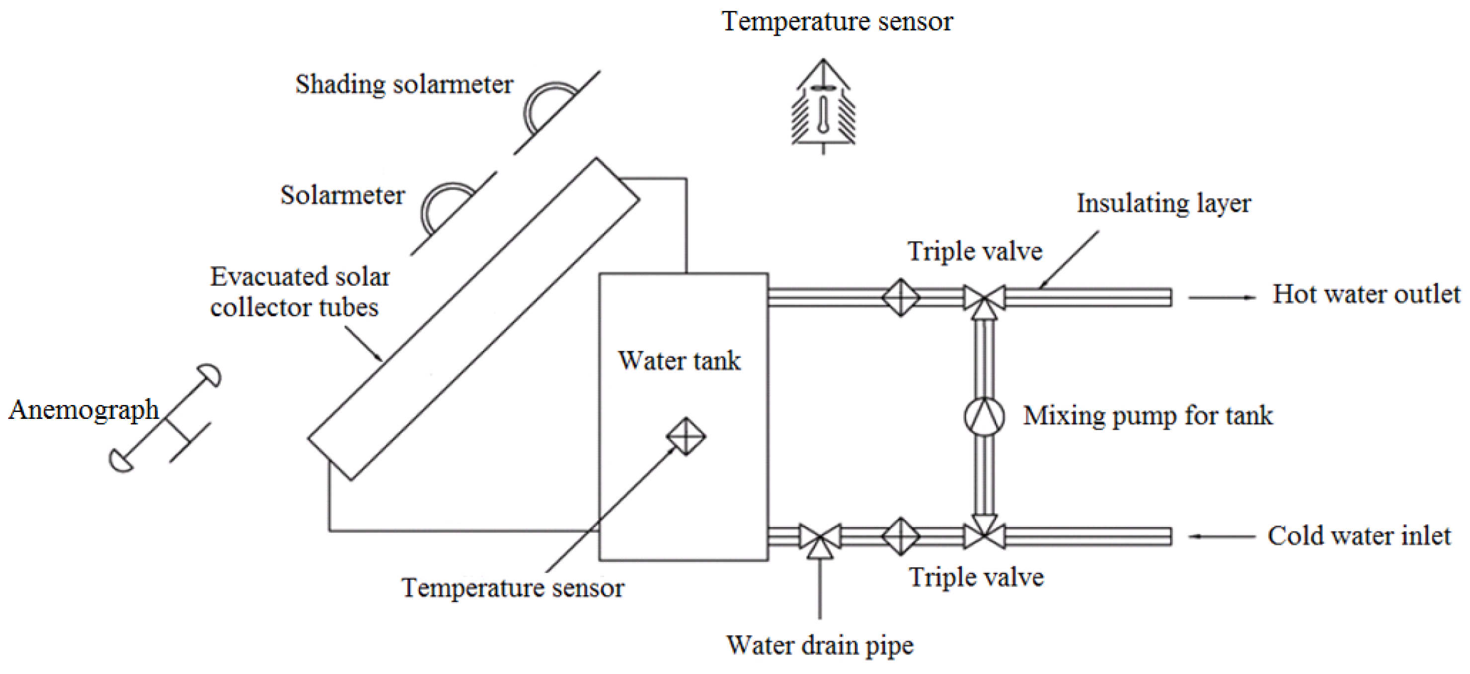
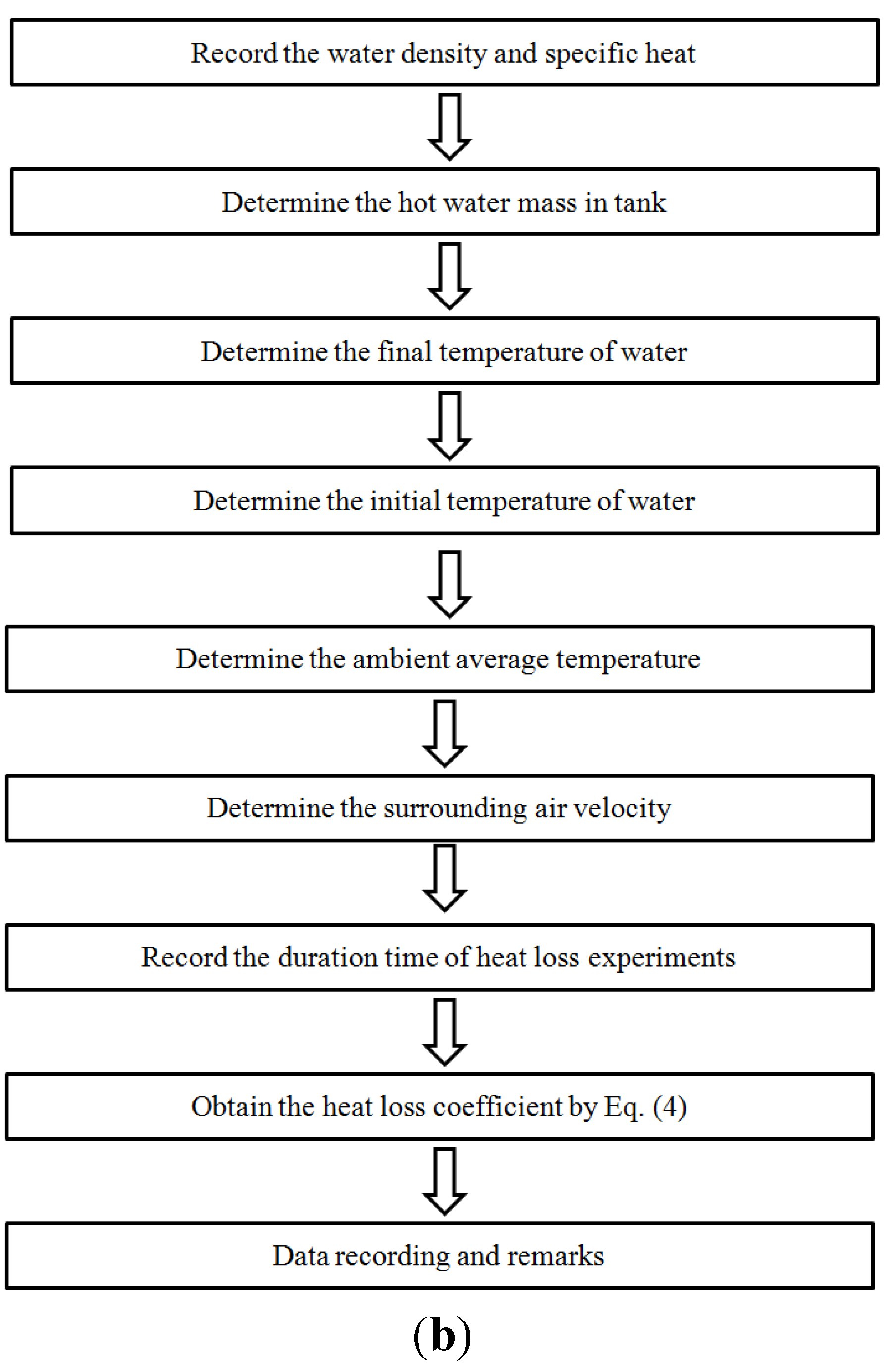
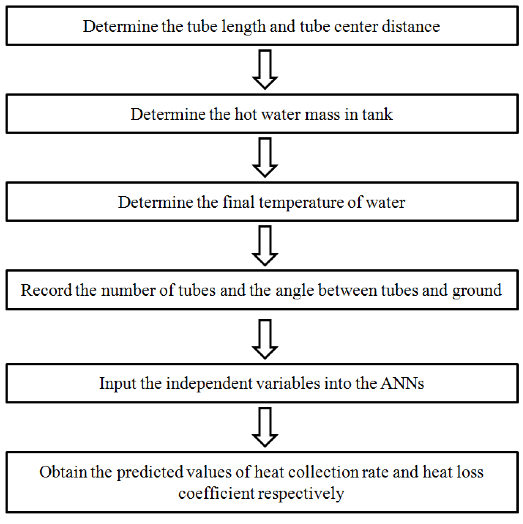
2.1. Experimental

According to the determination methods of independent and dependent variables in this research, 915 water-in-glass evacuated tube solar water heaters (in service for one year) were precisely determined by the “portable test instruments” and the PDT2013-1 (China Academy of Building Research, Beijing, China) detection device developed by the national center for quality supervision and testing of solar heating systems. Forty-eight PDT2013-1 detection devices were employed to measure the heat collection rate and heat loss coefficient (U_SL) simultaneously. Table 2 shows the statistical results of the experimental data.

Table 1. “Portable test instruments” for the determination of parameters of water-in-glass evacuated tube solar water heaters.

Parameters	Portable Test instruments	Accuracy	Picture
Final temperate of water	Digital thermoelectric thermometer	±0.5%
Hot water mass in tank	Electric platform scale	±1.0%
Diameter, tube center distance, tube length, collector area	Taper ZSH-3	±0.5%

Table 1. “Portable test instruments” for the determination of parameters of water-in-glass evacuated tube solar water heaters.

Parameters	Portable Test instruments	Accuracy	Picture
Final temperate of water	Digital thermoelectric thermometer	±0.5%
Hot water mass in tank	Electric platform scale	±1.0%
Diameter, tube center distance, tube length, collector area	Taper ZSH-3	±0.5%

Table 2. Descriptive statistic of the variables for 915 samples of in service water-in-glass evacuated tube solar water heaters.

Item	Tube Length (mm)	Number of Tubes	TCD (mm)	Tank Volume (kg)	Collector Area (m2)	Angle (°)	Final Temp. (°C)	HCR (MJ/m2)	HLC (W/(m3K))
Maximum	2200	64	151	403	8.24	85	62	11.3	13
Minimum	1600	5	60	70	1.27	30	46	6.7	8
Range	600	59	91	333	6.97	55	16	4.6	5
Average	1811	21	76.2	172	2.69	46	53	8.9	10
Standard deviation	87.8	5.8	5.11	47.0	0.73	3.89	2.0	0.48	0.77

Notes: Tube Center Distance (TCD), Temperature (Temp.), Heat Collection Rate (HCR), Heat Loss Coefficient (HLC).

Table 2. Descriptive statistic of the variables for 915 samples of in service water-in-glass evacuated tube solar water heaters.

Item	Tube Length (mm)	Number of Tubes	TCD (mm)	Tank Volume (kg)	Collector Area (m2)	Angle (°)	Final Temp. (°C)	HCR (MJ/m2)	HLC (W/(m3K))
Maximum	2200	64	151	403	8.24	85	62	11.3	13
Minimum	1600	5	60	70	1.27	30	46	6.7	8
Range	600	59	91	333	6.97	55	16	4.6	5
Average	1811	21	76.2	172	2.69	46	53	8.9	10
Standard deviation	87.8	5.8	5.11	47.0	0.73	3.89	2.0	0.48	0.77

Notes: Tube Center Distance (TCD), Temperature (Temp.), Heat Collection Rate (HCR), Heat Loss Coefficient (HLC).

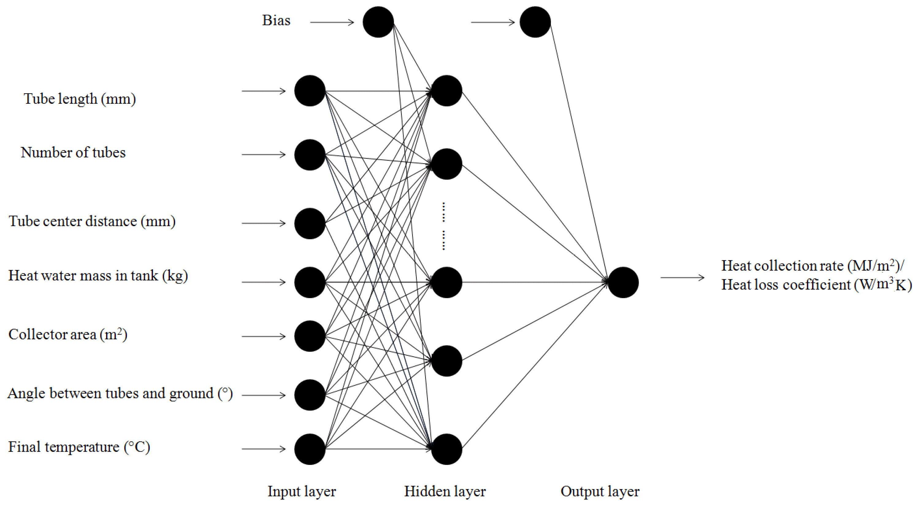
2.2. Artificial Neural Networks (ANNs)

ANNs [25,26,27] are strong machine learning approaches with functions of estimation and approximation based on input values. Interconnected neural networks are usually made up of neurons that can calculate values from inputs and adapt to different situations. Therefore, ANNs are widely used in numerical predictions and pattern recognitions. Currently, ANNs have become very popular in inferring a function from observation, especially when objects of study are too complex to be dealt with human brains. In our studies, two kinds of ANNs were used for model developments, multilayer feed-forward neural networks (MLFNs) and general regression neural network (GRNN).

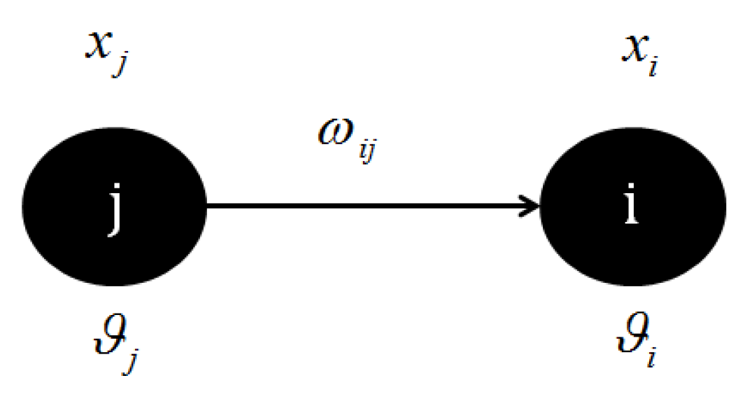
2.2.1. Multilayer Feed-Forward Neural Networks (MLFNs)

MLFN, trained with a back-propagation (BP) learning algorithm, is one of the most popular ANNs in scientific research [28,29,30]. Figure 2 is the schematic structure of an MLFN, with input, hidden, and output layers. Each single neuron interconnects with all neurons in the contiguous layer and each pair of connected neurons is connected via adaptable synaptic weights (Figure 3). As shown in Figure 3, the connection between the $i$th and $j$th neuron is characterized by the weight coefficient ${\omega }_{ij}$ and the threshold coefficients ${\vartheta }_i$ and ${\vartheta }_j$ [28]. The weight coefficient reflects the degree of importance of the given connection in the neural network. $x_i$ and $x_j$ are the output values of the $i$th and $j$th neurons, respectively. Knowledge is mainly stored as a set of connection weights, corresponding to synapse efficacy in human brain [31,32]. The process of training is the modification of connection weights until it satisfies users’ needs. During the training process, weights are adjusted in order to acquire the desired output [33].

Figure 2. Structure of the multilayer feed-forward neural network (MLFN).

Figure 2. Structure of the multilayer feed-forward neural network (MLFN).

Figure 3. Connection between neurons $i$ and $j$.

Figure 3. Connection between neurons $i$ and $j$.

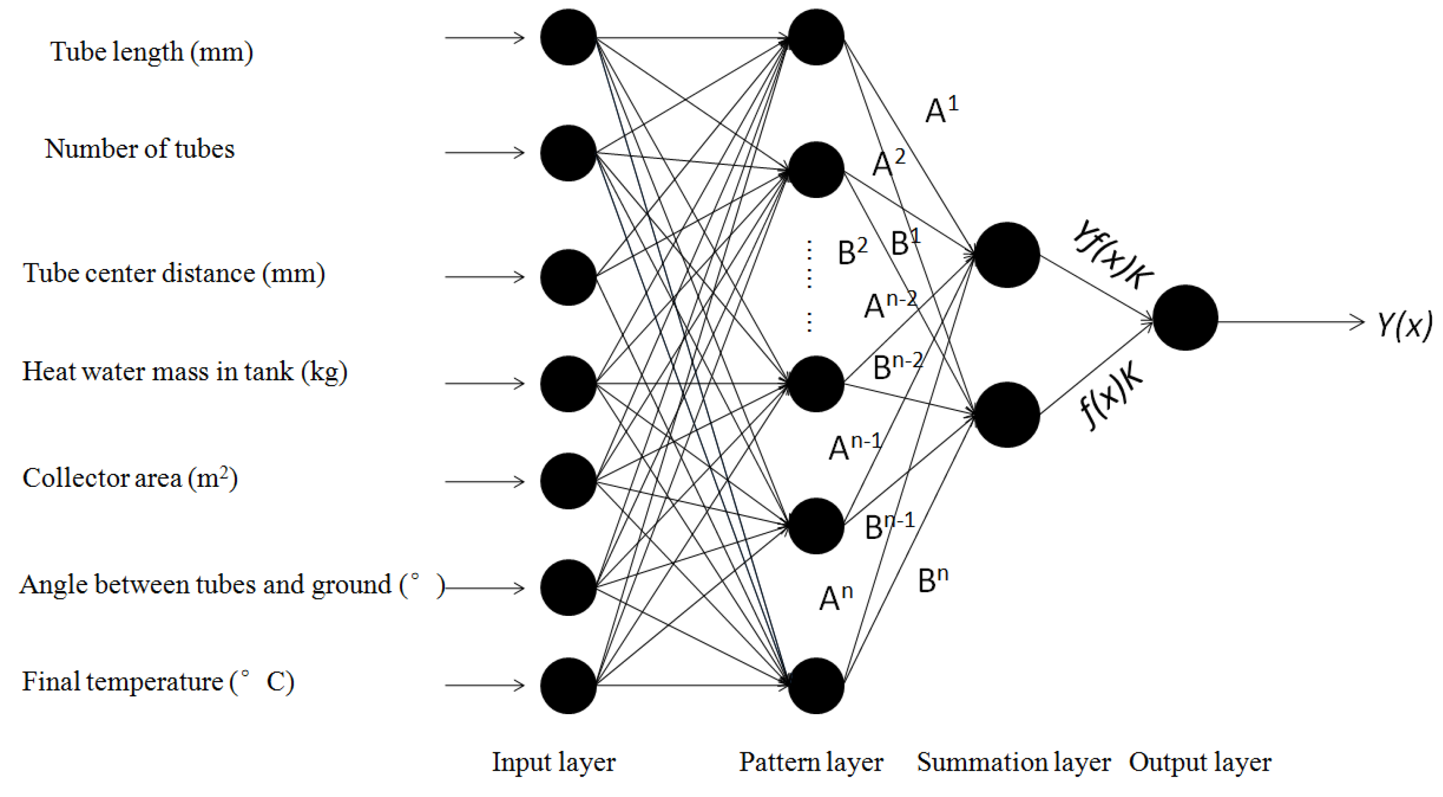
2.2.2. General Regression Neural Network (GRNN)

GRNN was firstly designed by Specht [34]. It has strong prediction capacity in prediction and pattern recognition [35]. The features of the GRNN are fast learning, consistency, and optimal regression with large number of samples [35]. Being similar to MLFN, GRNN consists of a series of interconnected neurons and layers. A typical GRNN has four layers: input, pattern, summation, and output, which are shown in Figure 4 [35]. The input layer keeps corresponding inputs and transfers input vector x to the pattern layer. The pattern layer consists of neurons for each training datum. Any test input applied to the network is first subtracted from the pattern layer neuron values. Either squares or absolute values of subtracts applied to exponential activation function will be summed. Results are transferred to the summation layer. Dot product of the pattern layer outputs and weights are added by summation layer neurons. As can be seen in Figure 4, weights are shown by A and B, and f(x)K denotes the weighted outputs of the pattern layer, where K is a Parzen window associated constant [26]. Yf(x)K denotes multiplication of pattern layer outputs and training data output Y values. At the output layer, f(x)K is divided by Yf(x)K to estimate the desired Y.

Figure 4. Structure of the general regression neural network (GRNN).

Figure 4. Structure of the general regression neural network (GRNN).

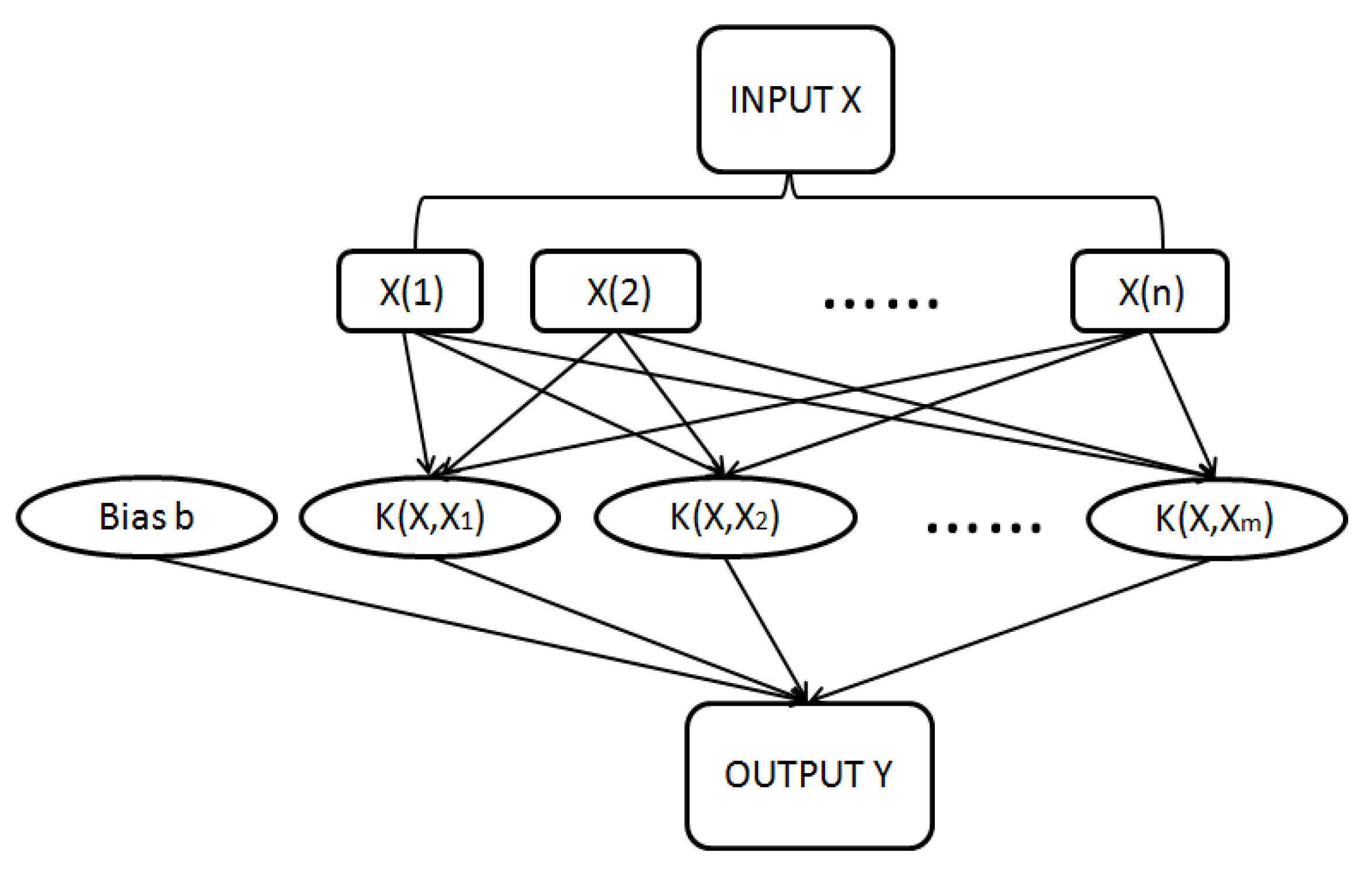
2.3. Support Vector Machine (SVM)

A support vector machine (SVM) is a novel machine learning algorithm based on statistical learning theory [36,37], which mainly uses the central concept called “kernel” for learning tasks. Kernel machines provide a modular framework that can be adapted to various tasks and domains with the use of different kernel functions (i.e., linear, polynomial, radial basis, or sigmoid) and the base algorithm [38]. Due to its principles, SVM has good performance in solving both prediction and classification problems. Figure 5 shows the main structure of SVM. The letter “K” represents kernels [39]. As can be seen from Figure 5, small subsets extracted from the training data by relevant algorithm consists of the SVM. For prediction and classification, choosing suitable kernel functions and appropriate parameters is important to get good prediction accuracy. With the development of computer science, there are currently many software packages that are helpful for us in developing the SVM [40,41].

Figure 5. Main structure of the support vector machine.

Figure 5. Main structure of the support vector machine.

3. Results and Discussion

3.1. Model Development

According to the determination capacity of “portable test instruments”, for an in service water-in-glass evacuated tube solar water heater, precise values of tube length, number of tubes, tube center distance, heat water mass in tank, collector area, final temperature and angle between tubes and ground can be easily obtained outdoors, while the heat collection rate and heat loss coefficient can only be determined by the detection device after being dismantled. To avoid complex disassembly and obtain the heat collection rate and heat loss coefficient in real time, here we aim at using machine learning techniques including ANNs and SVM to develop a series of prediction models for the heat collection rate and heat loss coefficient. Due to the large scale of data groups we acquired from experiments, the number of data groups in the testing set was large enough to help us evaluate the performance of the models. Also, if the number of data groups in the training set was not large enough (compared to that of the testing set), the training processes of models may had the risk of over-fitting. One of the empirical proportion settings for the testing set is lower than 20%, and we found that the setting of 15% proportion for the testing set to the total samples can ensure that a large number of experimental data groups (778 in total) were trained, and meanwhile, there was still a large number of data groups (137 in total) were tested. Therefore, 85% data groups, including the independent variables (tube length, number of tubes, tube center distance, heat water mass in tank, collector area, final temperature and angle between tubes and ground) and dependent variables (heat collection rate and heat loss coefficient) measured from 915 samples of in service water-in-glass evacuated tube solar water heater were set as the training set, while the remaining 15% were set as the testing set. The SVM model was developed by Matlab software. The ANN prediction models were constructed by the NeuralTools^® software (trial version, Palisade Corporation, New York, NY, USA) [42,43,44]. The GRNN and MLFN were chosen as the learning algorithms of ANNs.

Root mean square (RMS) error, required training time, and prediction accuracy (under the tolerances of 30%, 20%, and 10%, respectively) are used as indicators to measure the performances of the SVM and ANNs. Training times representing the required time for developing a complete learning machine were recorded during the training process of a model. The RMS errors were calculated from Equation (1) and the prediction accuracies were calculated from Equation (2):

$$\text{RMS error}=\sqrt{\frac{{\displaystyle {\sum }_{i=1}^n{(Z_i-O_i)}^2}}{n_{tot}}}$$

(1)

$$\text{Prediction accuracy}=\frac{n_{good}}{n_{tot}}\times 100\%,$$

(2)

where $Z_i$ is the predicted value, $O_i$ is the actual value, and $n_{tot}$ is the number of tested samples. $n_{good}$ is the number of tested samples with good predicted results under a certain tolerance.

The nodes of MLFN models were set from 2 to 39, from which we could find out the change regulation of the MLFN models when dealing with the development processes. Each model was trained for 20 times using different components of training and testing sets, then the mean RMS errors in testing, mean training times, and mean prediction accuracies were acquired. Table 3 and Table 4 show the development results for the prediction of heat collection rate and heat loss coefficient, respectively, using the mean RMS error in testing, mean training time, and mean prediction accuracy as the indicators for showing the performances of the models.

Table 3 shows that the mean RMS errors of the presented models are very close. The lowest mean RMS error exists in the MLFN with 12 nodes (0.14) and the second lowest mean RMS error exists in the MLFN with 3, 4, 7, 9, 10, 11, and 14 nodes respectively, which are all 0.15. The mean RMS errors of the SVM and GRNN are obviously higher than those of the MLFNs presented in Table 3 (0.29 and 0.33, respectively). In terms of the prediction accuracies, the mean prediction accuracies of the models are all 100% under the tolerance of 30%. Under the tolerance of 20%, most of the mean prediction accuracies of models are higher than 99.8%. When the tolerance is decreased to 10%, the MLFN with 3 and 12 nodes has the highest mean prediction accuracies among all models (98.33% and 98.57%, respectively). However, considering the mean training time of the models, the MLFN with 3 nodes has a significantly shorter mean training time. Comprehensively, the MLFN with 3 nodes (MLFN-3) can be considered as the best model for the prediction of heat collection rate due to its low RMS error, short training time, and high prediction accuracies under different tolerances.

Table 3. Results of prediction models for heat collection rate.

Model Type	Mean RMS Error in Testing	Mean Training Time	Mean Prediction Accuracy (30% tolerance)	Mean Prediction Accuracy (20% tolerance)	Mean Prediction Accuracy (10% tolerance)
SVM	0.29	0:00:10	100%	99.85%	95.11%
GRNN	0.33	0:00:14	100%	99.82%	94.42%
MLFN (2 Nodes)	0.17	0:05:57	100%	99.96%	97.08%
MLFN (3 Nodes)	0.15	0:07:12	100%	100%	98.33%
MLFN (4 Nodes)	0.15	0:08:35	100%	100%	97.21%
MLFN (5 Nodes)	0.17	0:10:03	100%	99.96%	97.03%
MLFN (6 Nodes)	0.17	0:11:23	100%	99.96%	96.89%
MLFN (7 Nodes)	0.15	0:13:39	100%	100%	97.31%
MLFN (8 Nodes)	0.19	0:14:35	100%	99.89%	96.54%
MLFN (9 Nodes)	0.15	0:15:45	100%	100%	97.18%
MLFN (10 Nodes)	0.15	0:17:56	100%	100%	97.62%
MLFN (11 Nodes)	0.15	0:19:10	100%	100%	97.19%
MLFN (12 Nodes)	0.14	0:20:47	100%	100%	98.57%
MLFN (13 Nodes)	0.16	0:21:51	100%	99.96%	97.01%
MLFN (14 Nodes)	0.15	0:23:12	100%	100%	97.31%
MLFN (15 Nodes)	0.17	0:24:19	100%	99.96%	96.92%
MLFN (16 Nodes)	0.19	0:26:05	100%	99.89%	96.43%
MLFN (17 Nodes)	0.16	0:29:05	100%	100%	95.72%
MLFN (18 Nodes)	0.23	0:28:50	100%	99.82%	96.33%
MLFN (19 Nodes)	0.19	0:30:20	100%	99.89%	96.57%
MLFN (20 Nodes)	0.2	0:32:26	100%	99.89%	95.92%
...	...	...	...	...	...
MLFN (39 Nodes)	0.22	1:07:44	100%	99.85%	95.41%

Table 3. Results of prediction models for heat collection rate.

Model Type	Mean RMS Error in Testing	Mean Training Time	Mean Prediction Accuracy (30% tolerance)	Mean Prediction Accuracy (20% tolerance)	Mean Prediction Accuracy (10% tolerance)
SVM	0.29	0:00:10	100%	99.85%	95.11%
GRNN	0.33	0:00:14	100%	99.82%	94.42%
MLFN (2 Nodes)	0.17	0:05:57	100%	99.96%	97.08%
MLFN (3 Nodes)	0.15	0:07:12	100%	100%	98.33%
MLFN (4 Nodes)	0.15	0:08:35	100%	100%	97.21%
MLFN (5 Nodes)	0.17	0:10:03	100%	99.96%	97.03%
MLFN (6 Nodes)	0.17	0:11:23	100%	99.96%	96.89%
MLFN (7 Nodes)	0.15	0:13:39	100%	100%	97.31%
MLFN (8 Nodes)	0.19	0:14:35	100%	99.89%	96.54%
MLFN (9 Nodes)	0.15	0:15:45	100%	100%	97.18%
MLFN (10 Nodes)	0.15	0:17:56	100%	100%	97.62%
MLFN (11 Nodes)	0.15	0:19:10	100%	100%	97.19%
MLFN (12 Nodes)	0.14	0:20:47	100%	100%	98.57%
MLFN (13 Nodes)	0.16	0:21:51	100%	99.96%	97.01%
MLFN (14 Nodes)	0.15	0:23:12	100%	100%	97.31%
MLFN (15 Nodes)	0.17	0:24:19	100%	99.96%	96.92%
MLFN (16 Nodes)	0.19	0:26:05	100%	99.89%	96.43%
MLFN (17 Nodes)	0.16	0:29:05	100%	100%	95.72%
MLFN (18 Nodes)	0.23	0:28:50	100%	99.82%	96.33%
MLFN (19 Nodes)	0.19	0:30:20	100%	99.89%	96.57%
MLFN (20 Nodes)	0.2	0:32:26	100%	99.89%	95.92%
...	...	...	...	...	...
MLFN (39 Nodes)	0.22	1:07:44	100%	99.85%	95.41%

Likewise, in terms of the prediction of heat loss coefficient, mean RMS errors are also similar among different models (Table 4). This shows that although the prediction accuracies of all the models presented in Table 4 are 100% under the tolerance of 30%, the GRNN has the highest prediction accuracies under the tolerances of 20% and 10%, respectively, and also has the significant advantage of comparatively low mean RMS error (0.71) and short mean training time (8 s). During our experiments, considering the RMS error, training time, and prediction accuracies under different tolerances, GRNN is regarded as the best prediction model for heat loss coefficient.

Table 4. Results of prediction models for heat loss coefficient.

Model Type	Mean RMS Error in Testing	Mean Training Time	Mean Prediction Accuracy (30% tolerance)	Mean Prediction Accuracy (20% tolerance)	Mean Prediction Accuracy (10% tolerance)
SVM	0.73	0:00:10	100%	98.81%	82.31%
GRNN	0.71	0:00:08	100%	99.38%	83.14%
MLFN (2 Nodes)	0.75	0:05:47	100%	98.44%	81.43%
MLFN (3 Nodes)	0.74	0:06:46	100%	98.51%	81.97%
MLFN (4 Nodes)	0.78	0:08:22	100%	98.17%	80.69%
MLFN (5 Nodes)	0.74	0:09:44	100%	98.61%	82.54%
MLFN (6 Nodes)	0.73	0:10:56	100%	98.76%	82.63%
MLFN (7 Nodes)	0.77	0:12:30	100%	98.13%	81.03%
MLFN (8 Nodes)	0.76	0:14:07	100%	98.44%	81.64%
MLFN (9 Nodes)	0.75	0:15:33	100%	98.65%	81.86%
MLFN (10 Nodes)	0.76	0:17:02	100%	98.43%	81.55%
MLFN (11 Nodes)	0.79	0:18:21	100%	97.97%	80.74%
MLFN (12 Nodes)	0.9	0:19:37	100%	93.32%	75.14%
MLFN (13 Nodes)	0.75	0:21:05	100%	98.66%	81.43%
MLFN (14 Nodes)	0.78	0:22:38	100%	98.04%	81.03%
MLFN (15 Nodes)	0.8	0:24:27	100%	97.36%	80.78%
MLFN (16 Nodes)	0.73	0:25:31	100%	98.35%	82.22%
MLFN (17 Nodes)	0.88	0:26:59	100%	93.93%	76.23%
MLFN (18 Nodes)	0.8	0:28:30	100%	96.41%	80.67%
MLFN (19 Nodes)	0.79	0:30:06	100%	97.43%	80.93%
MLFN (20 Nodes)	0.88	0:31:25	100%	93.86%	76.61%
...	...	...	...	...	...
MLFN (39 Nodes)	1.05	1:04:57	100%	89.61%	71.52%

Table 4. Results of prediction models for heat loss coefficient.

Model Type	Mean RMS Error in Testing	Mean Training Time	Mean Prediction Accuracy (30% tolerance)	Mean Prediction Accuracy (20% tolerance)	Mean Prediction Accuracy (10% tolerance)
SVM	0.73	0:00:10	100%	98.81%	82.31%
GRNN	0.71	0:00:08	100%	99.38%	83.14%
MLFN (2 Nodes)	0.75	0:05:47	100%	98.44%	81.43%
MLFN (3 Nodes)	0.74	0:06:46	100%	98.51%	81.97%
MLFN (4 Nodes)	0.78	0:08:22	100%	98.17%	80.69%
MLFN (5 Nodes)	0.74	0:09:44	100%	98.61%	82.54%
MLFN (6 Nodes)	0.73	0:10:56	100%	98.76%	82.63%
MLFN (7 Nodes)	0.77	0:12:30	100%	98.13%	81.03%
MLFN (8 Nodes)	0.76	0:14:07	100%	98.44%	81.64%
MLFN (9 Nodes)	0.75	0:15:33	100%	98.65%	81.86%
MLFN (10 Nodes)	0.76	0:17:02	100%	98.43%	81.55%
MLFN (11 Nodes)	0.79	0:18:21	100%	97.97%	80.74%
MLFN (12 Nodes)	0.9	0:19:37	100%	93.32%	75.14%
MLFN (13 Nodes)	0.75	0:21:05	100%	98.66%	81.43%
MLFN (14 Nodes)	0.78	0:22:38	100%	98.04%	81.03%
MLFN (15 Nodes)	0.8	0:24:27	100%	97.36%	80.78%
MLFN (16 Nodes)	0.73	0:25:31	100%	98.35%	82.22%
MLFN (17 Nodes)	0.88	0:26:59	100%	93.93%	76.23%
MLFN (18 Nodes)	0.8	0:28:30	100%	96.41%	80.67%
MLFN (19 Nodes)	0.79	0:30:06	100%	97.43%	80.93%
MLFN (20 Nodes)	0.88	0:31:25	100%	93.86%	76.61%
...	...	...	...	...	...
MLFN (39 Nodes)	1.05	1:04:57	100%	89.61%	71.52%

3.2. Model Analysis

To analyze the results of the best models for heat collection rate and heat loss coefficient, we should firstly divide the model development process of an ANN into two parts, the training and testing processes. The training process reveals the fitting results of an ANN, showing whether the training set was fitted properly and, at the same time, the capacity for recall of the model, which acts like the memory function of a human brain; the testing process reveals the prediction results of an ANN after training, showing whether the model can be applied to practical applications. Therefore, both training and testing results cannot be neglected when evaluating the precision and robustness of an ANN model.

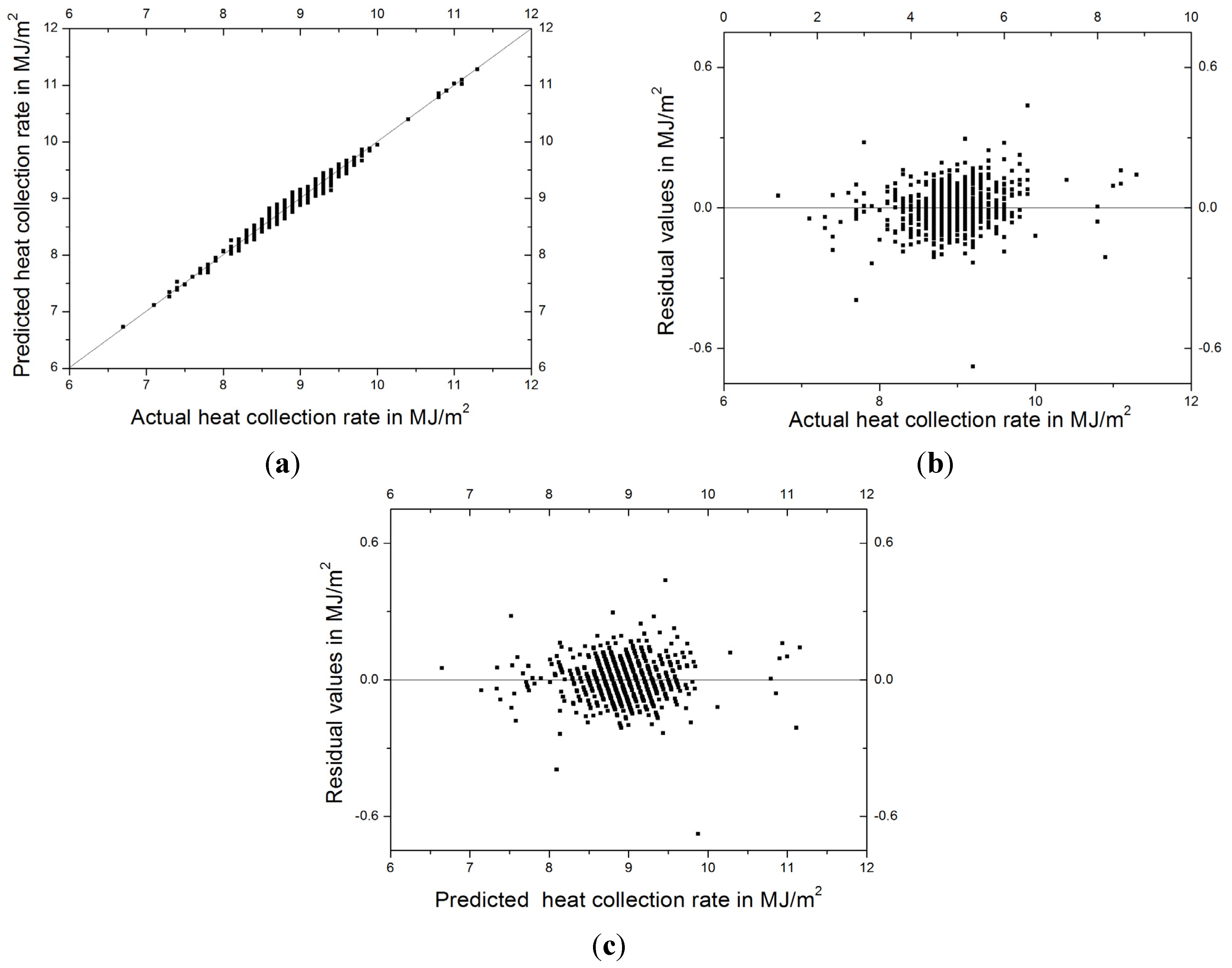
3.2.1. The MLFN-3 for Heat Collection Rate

Typical training results (Figure 6) and testing results (Figure 7) of the MLFN-3 for the prediction of heat collection rate are illustrated to show the robustness and precision of the model. It is significant that after the training process, the predicted values are close to the actual values (Figure 6a), which indicates that the MLFN-3 has a comparatively strong capacity for recalling the data in a training set. Residual values (Figure 6b,c) are also highly concentrated to zero, showing that the non-linear fitting results of the model are reliable.

In terms of the testing results, predicted values are also close to the actual values in the testing set (Figure 7a), indicating that the MLFN-3 has a very strong prediction capacity for heat collection rate. Residual values are also generally close to zero (Figure 7b,c). All these testing results prove that the MLFN-3 is a powerful tool to predict the heat collection rate based on the input of independent variables.

Figure 6. Training results of 778 samples using the MLFN-3 for the prediction of heat collection rate. (a) Predicted values versus actual values; (b) residual values versus actual values; (c) residual values versus predicted values.

Figure 6. Training results of 778 samples using the MLFN-3 for the prediction of heat collection rate. (a) Predicted values versus actual values; (b) residual values versus actual values; (c) residual values versus predicted values.

Figure 7. Testing results of 137 samples using the MLFN-3 for the prediction of heat collection rate. (a) Predicted values versus actual values; (b) residual values versus actual values; (c) residual values versus predicted values.

Figure 7. Testing results of 137 samples using the MLFN-3 for the prediction of heat collection rate. (a) Predicted values versus actual values; (b) residual values versus actual values; (c) residual values versus predicted values.

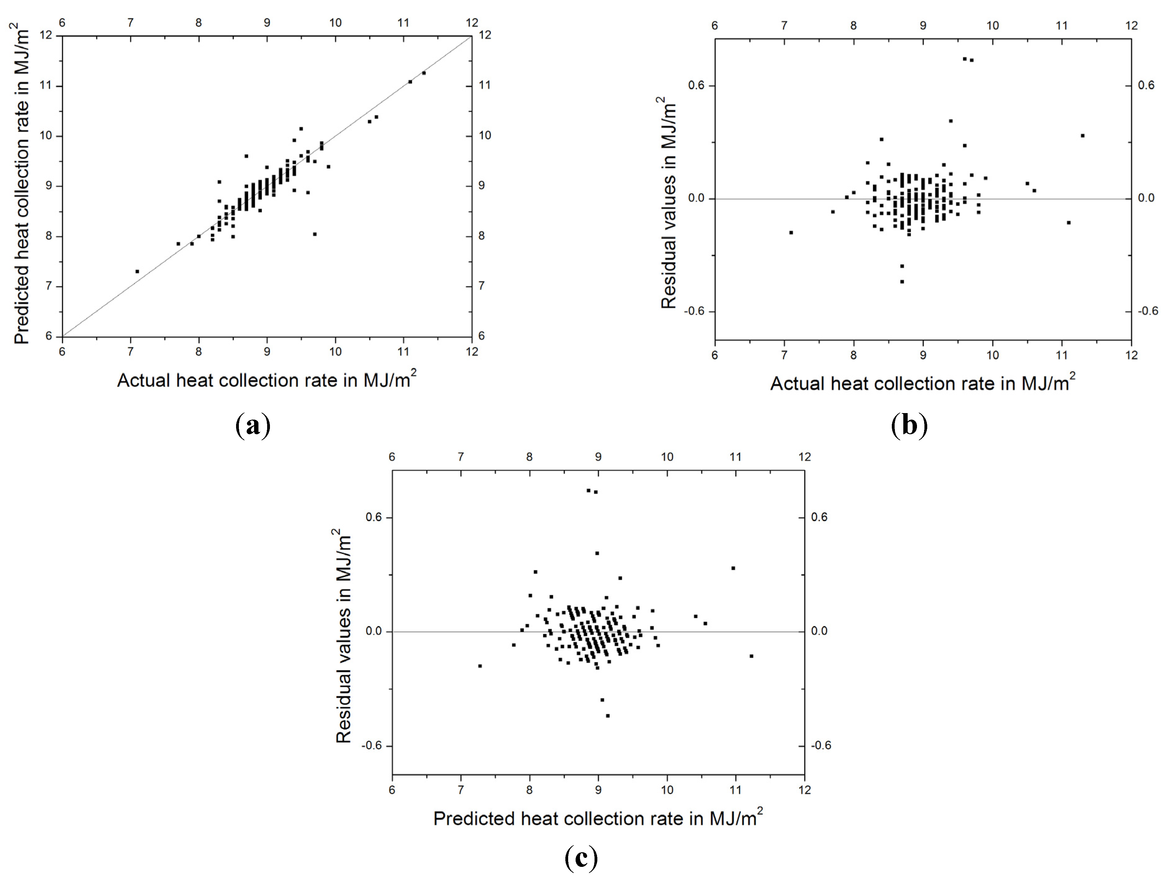
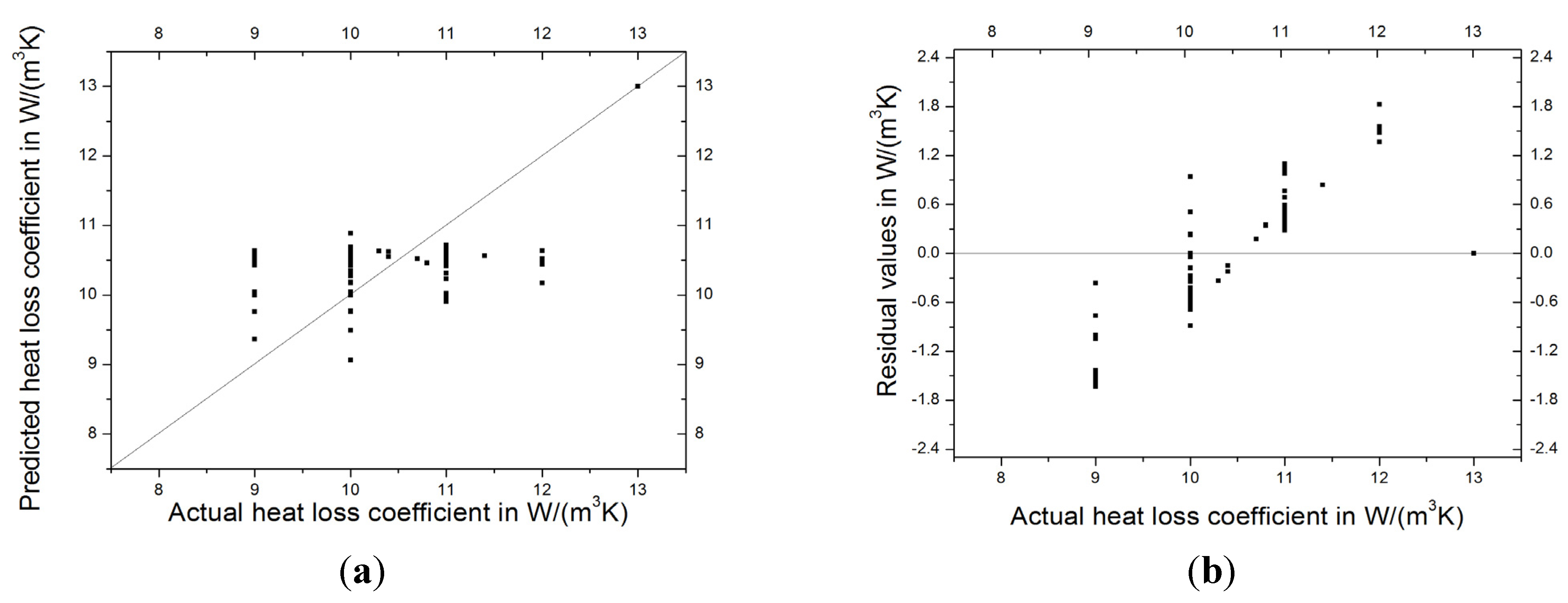
3.2.2. The GRNN for Heat Loss Coefficient

For the prediction of heat loss coefficient, the training results (Figure 8) and testing results (Figure 9) are illustrated to show the robustness and precision of the GRNN. It can be seen that after the training process, though there are some deviations, the predicted values generally correspond to the actual values in the training set (Figure 8a). The predicted values of heat loss coefficient are close to the actual values in the range between 10 and 11. The residual values (Figure 8b,c) also prove that more than one third of the residual values are very close to zero. In addition, although the rest of the predicted values (approximately two thirds of the values in the training set) have some deviation from their actual values, the deviations are all in a controllable range, with their residual values only ranging from −1.8 to 2.4. Therefore, the GRNN is also considered as a good model in a certain range of heat loss coefficient values.

In terms of the testing results, in the testing set, the predicted values (Figure 9a) are very close to the actual values when the values are in the range between 10 and 11. Above or below this range there may be some deviations when predicting. However, residual values (Figure 9b,c) show that the deviations are acceptable since all residual values are approximately ranging from −1.5 to 2.0. Also, in practical situations, most of the heat loss coefficient of water-in-glass evacuated tube solar water heater is in the exact range between 10 and 11 and the average of the values is 10 (as Table 2 shows). The RMS error (0.71) and prediction accuracy (100%) of the GRNN also show that the GRNN is a good predictor for heat loss coefficient. Therefore, in spite of the partial deviation phenomenon in the testing results, the GRNN is still acceptable and can be considered as the best model for the prediction of the heat loss coefficient.

Figure 8. Training results of 778 samples using the GRNN for the prediction of heat loss coefficient. (a) Predicted values versus actual values; (b) residual values versus actual values; (c) residual values versus predicted values.

Figure 8. Training results of 778 samples using the GRNN for the prediction of heat loss coefficient. (a) Predicted values versus actual values; (b) residual values versus actual values; (c) residual values versus predicted values.

Figure 9. Testing results of 137 samples using the GRNN for the prediction of heat loss coefficient. (a) Predicted values versus actual values; (b) Residual values versus actual values; (c) Residual values versus predicted values.

Figure 9. Testing results of 137 samples using the GRNN for the prediction of heat loss coefficient. (a) Predicted values versus actual values; (b) Residual values versus actual values; (c) Residual values versus predicted values.

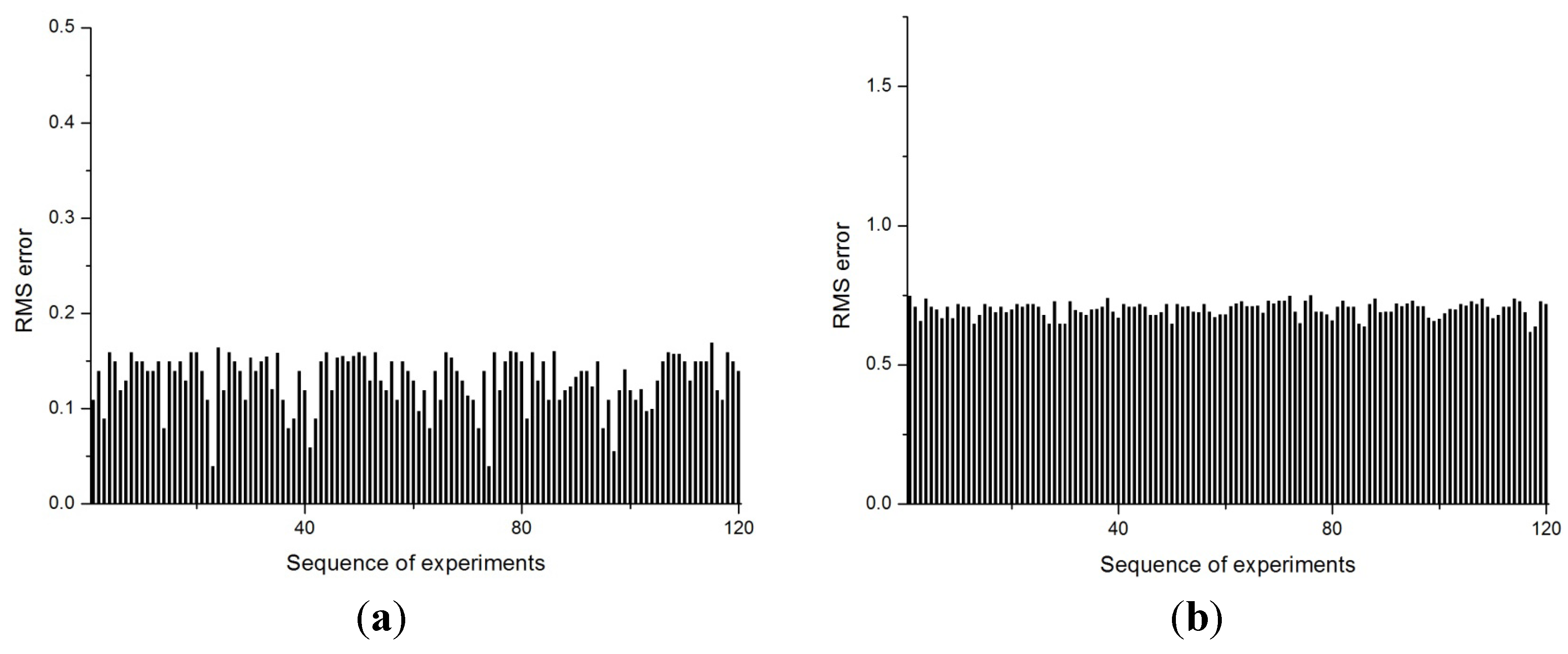
3.3. Robustness Analysis

According to the principles of the ANN algorithm, the initial values created in the “hidden box” are chosen at random. Therefore, the reproducibility of an ANN cannot be neglected. Since confirming the reproducibility of an ANN requires a large number of repeated experiments, here we test the reproducibility MLFN-3 and GRNN for the prediction of heat collection rate and heat loss coefficient via repeating the same experiments. One hundred twenty repeated experiments were done in order to see the fluctuations of the ANNs. Repeated experiments of the MLFN-3 for the prediction of heat collection rate (Figure 10a) show that although fluctuation exists in the change of RMS errors, there is no “sudden jump” during the 120 repeated experiments. All RMS errors of the model are below 0.18. Results show that the MLFN-3 is robust for the prediction of heat collection rate. Repeated experiments of the GRNN for the prediction of heat loss coefficient (Figure 10b) show that the GRNN is highly robust during repeated experiments, with only tiny fluctuations. Results show that the GRNN for the prediction of heat loss coefficient has an excellent reproducibility.

Figure 10. Repeated experiments of (a) the MLFN-3 for the prediction of heat collection rate and (b) the GRNN for the prediction of heat loss coefficient.

Figure 10. Repeated experiments of (a) the MLFN-3 for the prediction of heat collection rate and (b) the GRNN for the prediction of heat loss coefficient.

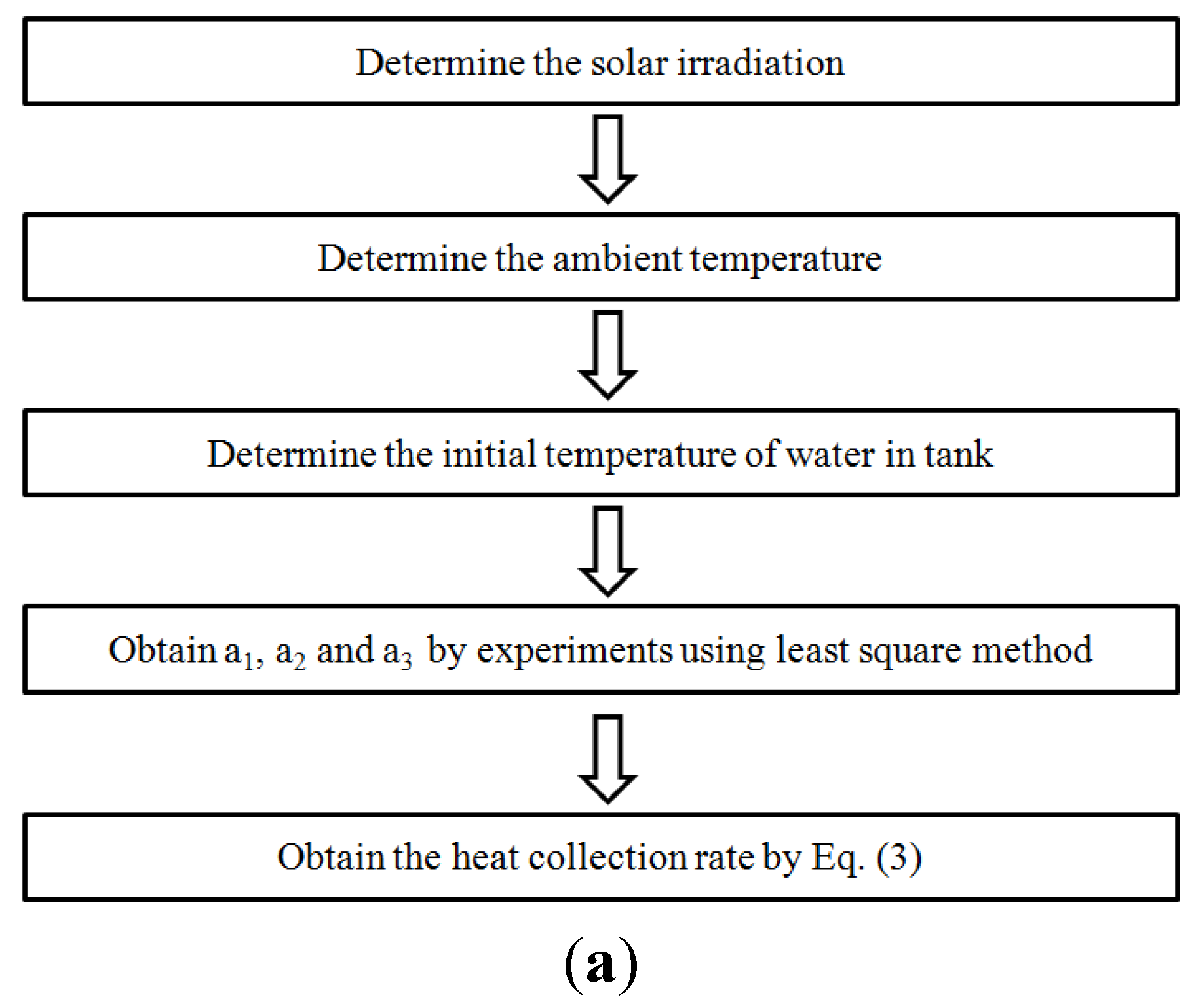
3.4. Comparison with Conventional Methods

According to conventional methods for the determination of heat collection rate and heat loss coefficient, technicians should accomplish a series of steps using the detection devices (Figure 11). The water-in-glass evacuated tube solar water heaters should be dismantled at first. However, for the determination for the in service heaters, the disassembly of the heater is highly inconvenient and will cause damage to instruments. What is worse, a completed conventional determination process requires at least 15 days. After a series of complicated determination processes, the heat collection rate and heat loss coefficient should be obtained by Equations (3) and (4), respectively:

$$q_s=\frac{a_{1}H+a_2(t_a-t_i)+a_3}{S}$$

(3)

$$U_s=\frac{{\rho }_w{C}_{p,w}{V}_s}{V\mathrm{\Delta }\tau }\ln \left[\frac{t_{is}-t_{as(av)}}{t_{fs}-t_{as(av)}}\right]$$

(4)

where q_s is the heat collection rate; H is the amount of solar radiation; t_a is the ambient temperature; t_i is the initial temperature of water in tank; S is the area of tubes and a₁, a₂ and a₃ are the coefficients; U_s is the heat loss coefficient according to the ISO 9459-2 [45]; ρ_w is the water density; C_p,w is the specific heat of water; V_s is the heat water mass in the tank; t_is is the initial temperature of water; t_fs is the final temperature of water; t_as(av) is the ambient average temperature; V is the volume of water; and ∆τ is the duration time of heat loss coefficient experiments.

To revolutionize the determination method, the novel method we propose here can avoid the disassembly to the heaters and meanwhile save time. The determination process using our novel method is presented in Figure 12, showing that the independent variables in our study can be inputted into the ANNs after being obtained by “portable test instruments”. The precise predicted results of heat collection rate and heat loss coefficient can be obtained precisely from the output of the ANNs. The use of “portable test instruments” in combination with ANNs can save time and give highly precise predicted results. However, this new method was only suitable for water-in-glass evacuated tube solar water heaters from one Chinese company. The model here could be employed for the prediction of the heat collection rate under the conditions of the Chinese standard GB/T 19141 [23].

Figure 11. Flow chart of the conventional method for determining (a) heat collection and (b) heat loss coefficient.

Figure 11. Flow chart of the conventional method for determining (a) heat collection and (b) heat loss coefficient.

Figure 12. Flow chart of the novel method using “portable test instruments” combined with ANNs for determining heat collection rate and heat loss coefficient.

Figure 12. Flow chart of the novel method using “portable test instruments” combined with ANNs for determining heat collection rate and heat loss coefficient.

4. Conclusions

Here, the best prediction models for heat collection rate and heat loss coefficient of water-in-glass evacuated tube solar water heaters are proposed after detailed model development and analysis. Results show that the MLFN-3 has the best prediction results for heat collection rate and the GRNN has the best prediction for heat loss coefficient due to their low RMS errors, short training times, and high prediction accuracies. In practical applications, the determination of heat collection rate and heat loss coefficient can be undertaken outdoors using “portable test instruments”. Data of independent variables obtained by “portable test instruments” can be inputted into the ANNs and the precise predicted values of heat collection rate and heat loss coefficient can be obtained rapidly in the output of the models. Therefore, using our novel determination techniques with the combination of “portable test instruments” and ANNs can acquire the heat collection rate and heat loss coefficient easily and quickly. However, ANNs are developed totally based on the training of experimental data, which may neglect the inner principles and theories between the independent and dependent variables, which is what we call the “black box.” Although it is a major advantage of ANNs, it leads to difficulties in studying the exact causalities between the independent and dependent variables, which may also be hard for us to remove unnecessary noise when training. Future studies may find it difficult to optimize the design of assembly conditions of water-in-glass evacuated tube solar water heaters using ANN methods. Fortunately, with a large-scale experimental data like the large sample size in this study, noise can be eliminated with a proper training process, ensuring good predicted results. With the help of this study, the determinations of heat collection rate and heat loss coefficient no longer need to be undertaken in a laboratory after dismantling the solar water heater, which can avoid probable damage to related instruments and at the same time enormously reduce manpower, experimental time, and unnecessary operations. Further studies will be aimed at two explorations: (i) developing a robust software in both personal computer (PC) and mobile phone platforms, in order to assist the practical measurements using the novel method; and (ii) optimizing the assembly conditions of water-in-glass evacuated tube solar water heaters with higher heat collection rates and lower heat loss coefficients, using high-throughput screening based on ANNs. However, the developed models were only suitable for water-in-glass evacuated tube solar water heaters from one Chinese company. The model here cannot be used for the prediction of the heat collection rate under other conditions than the ones stated within Chinese standard GB/T 19141.

References

1. Mekhilef, S.; Saidur, R.; Safari, A. A review on solar energy use in industries. Renew. Sustain. Energy Rev. 2011, 15, 1777–1790. [Google Scholar] [CrossRef]
2. Kalogirou, S. The potential of solar industrial process heat applications. Appl. Energy 2003, 76, 337–361. [Google Scholar] [CrossRef]
3. Morrison, G.L.; Tran, N.H.; McKenzie, D.R.; Onley, I.C.; Harding, G.L.; Collins, R.E. Long term performance of evacuated tubular solar water heaters in Sydney, Australia. Sol. Energy 1984, 32, 785–791. [Google Scholar] [CrossRef]
4. Shah, L.J.; Furbo, S. Theoretical flow investigations of an all glass evacuated tubular collector. Sol. Energy 2007, 81, 822–888. [Google Scholar] [CrossRef]
5. Liu, Z.H.; Hu, R.L.; Lu, L.; Zhao, F.; Xiao, H.S. Thermal performance of an open thermosyphon using nanofluid for evacuated tubular high temperature air solar collector. Energy Convers. Manag. 2013, 73, 135–143. [Google Scholar] [CrossRef]
6. Tang, R.S.; Li, Z.M.; Xia, C.F.; Lan, Q. Assessment of uncertainty in heat loss coefficient of all glass evacuated solar tubes testing. Energy Convers. Manag. 2006, 47, 60–67. [Google Scholar] [CrossRef]
7. Liu, Y.M.; Chung, K.M.; Chang, K.C.; Lee, T.S. Performance of thermosyphon solar water heaters in series. Energies 2012, 5, 3266–3278. [Google Scholar] [CrossRef]
8. Morrison, G.L.; Budihardjo, I.; Behnia, M. Water-in-glass evacuated tube solar water heaters. Sol. Energy 2014, 76, 135–140. [Google Scholar] [CrossRef]
9. Pei, G.; Li, G.; Zhou, X.; Ji, J.; Su, Y. Comparative experimental analysis of the thermal performance of evacuated tube solar water heater systems with and without a mini-compound parabolic concentrating (CPC) reflector (C < 1). Energies 2012, 5, 911–924. [Google Scholar]
10. Lin, W.M.; Chang, K.C.; Liu, Y.M.; Chung, K.M. Field surveys of non-residential solar water heating systems in Taiwan. Energies 2012, 5, 258–269. [Google Scholar] [CrossRef]
11. Çomaklı, K.; Çakır, U.; Kaya, M.; Bakirci, K. The relation of collector and storage tank size in solar heating systems. Energy Convers. Manag. 2012, 63, 112–117. [Google Scholar] [CrossRef]
12. Govind, N.K.; Shireesh, B.K.; Satanu, B. Optimization of solar water heating system through water replenishment. Energy Convers. Manag. 2009, 50, 837–846. [Google Scholar]
13. Tang, R.; Gao, W.; Yu, Y.; Chen, H. Optimal tilt-angles of all-glass evacuated tube solar collectors. Energy 2009, 34, 1387–1395. [Google Scholar] [CrossRef]
14. Wang, P.Y.; Guan, H.Y.; Liu, Z.H.; Wang, G.S.; Zhao, F.; Xiao, H.S. High temperature collecting performance of a new all-glass evacuated tubular solar air heater with U-shaped tube heat exchanger. Energy Convers. Manag. 2014, 77, 315–323. [Google Scholar] [CrossRef]
15. Porras-Prieto, C.J.; Mazarrón, F.R.; DelosMozos, V.; García, J.L. Influence of required tank water temperature on the energy performance and water withdrawal potential of a solar water heating system equipped with a heat pipe evacuated tube collector. Sol. Energy 2014, 110, 365–677. [Google Scholar] [CrossRef]
16. Zhang, X.; You, S.; Xu, W.; Wang, M.; He, T.; Zheng, X. Experimental investigation of the higher coefficient of thermal performance for water-in-glass evacuated tube solar water heaters in China. Energy Convers. Manag. 2014, 78, 386–392. [Google Scholar] [CrossRef]
17. Kalogirou, S.A.; Panteliou, S.; Dentsoras, A. Modelling of solar domestic water-heating systems using artificial neural-networks. Sol. Energy 1999, 65, 335–342. [Google Scholar] [CrossRef]
18. Kalogirou, S.A. Prediction of flat-plate collector performance parameters using artificial neural network. Sol. Energy 2006, 80, 248–259. [Google Scholar] [CrossRef]
19. Kalogirou, S.A.; Mathioulakis, E.; Belessiotis, V. Artificial neural networks for the performance prediction of large solar systems. Renew. Energy 2014, 63, 90–97. [Google Scholar] [CrossRef]
20. Kalogirou, S.A.; Panteliou, S. Thermosiphon solar domestic water heating systems long-term performance prediction using artificial neural networks. Sol. Energy 2000, 69, 163–174. [Google Scholar] [CrossRef]
21. Kalogirou, S.A.; Neocleous, C.; Schizas, C. Artificial neural networks for modelling the starting-up of a solar steam generator. Appl. Energy 1998, 60, 89–100. [Google Scholar] [CrossRef]
22. Lecoeuche, S.; Lalot, S. Prediction of the daily performance of solar collectors. Int. Commun. Heat Mass Transf. 2005, 32, 603–611. [Google Scholar] [CrossRef]
23. Specification of Domestic Solar Water Heating Systems; GB/T 19141; Standard Press: Beijing, China, 2011. (In Chinese)
24. Hugo, A.; Zmeureanu, R. Residential solar-based seasonal thermal storage systems in cold climates: Building envelope and thermal storage. Energies 2012, 5, 3972–3985. [Google Scholar] [CrossRef]
25. Wang, F.; Mi, Z.; Su, S.; Zhao, H. Short-term solar irradiance forecasting model based on artificial neural network using statistical feature parameters. Energies 2012, 5, 1355–1370. [Google Scholar] [CrossRef]
26. Kandananond, K. Forecasting electricity demand in Thailand with an artificial neural network approach. Energies 2011, 4, 1246–1257. [Google Scholar] [CrossRef]
27. Rashidi, M.M.; Ali, M.; Freidoonimehr, N.; Nazari, F. Parametric analysis and optimization of entropy generation in unsteady MHD flow over a stretching rotating disk using artificial neural network and particle swarm optimization algorithm. Energy 2013, 55, 497–510. [Google Scholar] [CrossRef]
28. Svozil, D.; Kvasnicka, V.; Pospichal, J. Introduction to multi-layer feed-forward neural networks. Chemom. Intell. Lab. Syst. 1997, 39, 43–62. [Google Scholar] [CrossRef]
29. Johansson, E.M.; Dowla, F.U.; Goodman, D.M. Backpropagation learning for multilayer feed-forward neural networks using the conjugate gradient method. Int. J. Neural Syst. 1991, 2, 291–301. [Google Scholar] [CrossRef]
30. Guo, Z.; Zhao, W.; Lu, H.; Wang, J. Multi-step forecasting for wind speed using a modified EMD-based artificial neural network model. Renew. Energy 2012, 37, 241–249. [Google Scholar] [CrossRef]
31. Kalogirou, S.A. Applications of artificial neural-networks for energy systems. Appl. Energy 2000, 67, 17–35. [Google Scholar] [CrossRef]
32. Kalogirou, S.A. Artificial neural networks in renewable energy systems applications: A review. Renew. Sustain. Energy Rev. 2001, 5, 373–401. [Google Scholar] [CrossRef]
33. Kalogirou, S.A.; Sencan, A. Artificial Intelligence Techniques in Solar Energy Applications. Available online: http://www.intechopen.com/articles/show/title/artificial-intelligence-techniques-in-solar-energy-applications (accessed on 17 August 2015).
34. Specht, D.F. A general regression neural network. IEEE. Trans. Neural. Netw. 1991, 2, 568–576. [Google Scholar] [CrossRef] [PubMed]
35. Kandirmaz, H.M.; Kaba, K.; Avci, M. Estimation of monthly sunshine duration in Turkey using artificial neural networks. Int. J. Photoenergy 2014, 14, 9–10. [Google Scholar] [CrossRef]
36. Deng, N.; Tian, Y.; Zhang, C. Support Vector Machines: Optimization Based Theory, Algorithms, and Extensions, 2nd ed.; Chapman & Hall/CRC: Boca Raton, FL, USA, 2012; pp. 154–162. [Google Scholar]
37. Zhong, X.; Li, J.; Dou, H.; Deng, S.; Wang, G.; Jiang, Y.; Yan, F. Fuzzy nonlinear proximal support vector machine for land extraction based on remote sensing image. PLoS ONE 2013, 8, 694–698. [Google Scholar] [CrossRef]
38. Jian, L.; Weikang, K.; Jiangbo, S.; Ke, W.; Weikui, W.; Weipu, Z.; Zhoumo, Z. Determination of corrosion types from electrochemical noise by artificial neural networks. Int. J. Electrochem. Sci. 2013, 8, 2365–2377. [Google Scholar]
39. Kim, D.W.; Lee, K.; Lee, D.; Lee, K.H. A kernel-based subtractive clustering method. Pattern Recognit. Lett. 2005, 26, 879–891. [Google Scholar] [CrossRef]
40. Fan, R.E.; Chang, K.W.; Hsieh, C.J.; Wang, X.R.; Lin, C.J. LIBLINEAR: A library for large linear classification. J. Mach. Learn. Res. 2008, 9, 1871–1874. [Google Scholar]
41. Guo, Q.; Liu, Y. ModEco: An integrated software package for ecological niche modeling. Ecography 2010, 33, 637–642. [Google Scholar] [CrossRef]
42. Vouk, D.; Malus, D.; Halkijevic, I. Neural networks in economic analyses of wastewater systems. Expert Syst. Appl. 2011, 38, 10031–10035. [Google Scholar] [CrossRef]
43. Saadah, L.M.; Chedid, F.D.; Sohail, M.R.; Nazzal, Y.M.; Al-Kaabi, M.R.; Rahmani, A.Y. Palivizumab prophylaxis during nosocomial outbreaks of respiratory syncytial virus in a neonatal intensive care unit: Predicting effectiveness with an artificial neural network model. Pharmacother. J. Hum. Pharmacol. Drug Ther. 2014, 34, 251–259. [Google Scholar] [CrossRef] [PubMed]
44. Goh, Y.M.; Binte Sa’adon, N.F. Cognitive Factors Influencing Safety Behavior at Height: A Multimethod Exploratory Study. J. Constr. Eng. Manag. 2015, 9, 107–112. [Google Scholar] [CrossRef]
45. Solar Heating—Domestic Water Heating Systems—Part 2: Outdoor Test Methods for System Performance Characterization and Yearly Performance Prediction of Solar-Only Systems; ISO 9459-2; ISO: Geneva, Switzerland, 1995.