Linearization and Input-Output Decoupling for Nonlinear Control of Proton Exchange Membrane Fuel Cells

Abstract

This paper presents a nonlinear control strategy utilizing the linearization and input-output decoupling approach for a nonlinear dynamic model of proton exchange membrane fuel cells (PEMFCs). The multiple-input single-output (MISO) nonlinear model of the PEMFC is derived first. The dynamic model is then transformed into a multiple-input multiple-output (MIMO) square system by adding additional states and outputs so that the linearization and input-output decoupling approach can be directly applied. A PI tracking control is also introduced to the state feedback control law in order to reduce the steady-state errors due to parameter uncertainty. This paper also proposes an adaptive genetic algorithm (AGA) for the multi-objective optimization design of the tracking controller. The comprehensive results of simulation demonstrate that the PEMFC with nonlinear control has better transient and steady-state performance compared to conventional linear techniques.

1. Introduction

Nowadays, the popular renewable energy sources include wind power, solar power generation and fuel cells. However, wind power and solar power are usually affected by external environmental factors, which cause the instability of the power generator output. In contrast to wind and solar power, fuel cells generate electricity stably and are less susceptible to external environment factors [1,2]. The fuel cell is similar to a traditional battery transforming the chemical energy of an active substance into electrical energy. It is not a rechargeable battery, that it has to recharge to continuously function, but rather by adding a fuel and oxidizer it produces an electrochemical reaction that directly transforms chemical into electrical energy. Therefore, it has many desirable features such as a high power conversion efficiency (40%–60%), low noise (no operating machinery), low pollution (the byproduct is water), extensive choice of feeds (hydrogen, methanol, natural gas, etc.), and multipurpose applications (electric vehicles, power plants, etc.) [3–5].

A PEMFC is a nonlinear and strongly coupled dynamic system. As the driven load changes, the output current changes and the electrochemical reaction is simultaneously accelerated. If the inlet flow rate of oxygen in the cathode is too low, the output power of PEMFC system would be decreased because of a lack of oxygen, which is known as starvation. In order to generate a reliable and efficient power response and prevent detrimental degradation of the stack voltage, it is very important to design an effective control strategy to achieve optimal oxygen and hydrogen inlet flow rates control.

Many control strategies been adopted nowadays for controlling PEMFC systems. Golbert [6] used predictive control to satisfy the power needs based on fuel cell model linearization. According to the experimental data, Almeda [7] proposed an artificial neural network control method to control fuel cell output voltage and optimize the system parameters. Schumacher [8] proposed a method for PEMFC water management using fuzzy control. Pukrushpan [9,10] used feed-forward and feedback strategies to control the flow rate of the compressor in the air supply system of a PEMFC. However, the existing control approaches were based on linear models which were linearized at a specific operating point. When they encounter a large range of disturbances such linear control approaches have difficulties in achieving satisfactory performance, therefore, an accurate nonlinear dynamic model for PEMFC and an advanced controller design approach considering the nonlinearity and uncertainty are urgently needed.

State feedback linearization and input-output decoupling for nonlinear dynamic models have been widely used to enhance transient performance [11–13]. The approach of using feedback linearization to obtain a linear model is valid for a broader operating range, and under certain circumstances this linearization is even valid for the whole operating range. Moreover, the input-output decoupling technique is utilized such that each of the outputs is independently controlled by one and only one of the newly defined inputs. In this paper, a MIMO dynamic nonlinear model of a PEMFC that is appropriate for developing a nonlinear controller based on the linearization and input-output decoupling approach is presented. The state feedback exact linearization [12,13] is applied to design the control law, based directly on the nonlinear dynamic PEMFC model. The control law obtained from the state feedback exact linearization is expected to enhance the transient performance in the presence of large disturbances.

2. PEMFC Dynamic Model

The working process of a PEMFC is accompanied with liquid/vapor/gas mixed flow transportation, heat conduction and electrochemical reactions. In order to simplify the analysis, several assumptions are made as listed below:

(1)

The governing equation is the Nernst equation.

(2)

The entire PEMFC is at the same operating temperature.

(3)

The entire gas is the ideal gas at a relative humidity of 100%.

(4)

The electrolyte membrane is of a high proton conductivity.

(5)

The gases are completely pure hydrogen and oxygen.

The nonlinear dynamic model developed in this paper is based on the FC models presented in [14–17].

2.1. Output Voltage Model

The output voltage of a single fuel cell, according to the Nernst equation, is formulated as:

$$V_{\text{FC}}=E_{\text{nernst}}-V_{\text{act}}-V_{\text{ohmic}}-V_{\text{con}}$$

(1)

In the above equation E_Nernst denotes the thermodynamic potential, that is the reversible voltage of the cell, represented by:

$$E_{\text{Nernst}}=\frac{\mathrm{\Delta }G}{2\text{F}}+\frac{\mathrm{\Delta }S}{2\text{F}}(T-T_0)+\frac{R_{0}T}{2\text{F}}\left[ln(P_{{\text{H}}_2})+\frac{1}{2}ln(P_{{\text{O}}_2})\right]$$

(2)

where ΔG (J/mol) denotes Gibb's free energy change, F the Faraday's constant (96,487 C/mol), ΔS (J/mol) the standard mole entropy change, R₀ the universal gas constant (8.315 J/mol K), P_H2 and P_O2 are the partial pressures of hydrogen and oxygen respectively, T and T₀ are the cell's operating temperature and reference temperature respectively.

V_act represents the activation voltage drop, which is the polarization arising from the cathode and anode, given as:

$$V_{\text{act}}=-[{\xi }_1+{\xi }_2\cdot T+{\xi }_3\cdot T\cdot ln(c_{{\text{O}}_2})+{\xi }_4\cdot T\cdot ln(i)]$$

(3)

where i represents the cell's operation current, and ξ_j the semi-empirical coefficients, defined as:

$${\xi }_1=-0.948$$

(4)

$${\xi }_2=286\times {10}^{-5}+20\times {10}^{-5}\times lnA+4.3\times {10}^{-5}\times ln{c}_{{\text{H}}_2}={\xi }_{\mathrm{2\_1}}+{\xi }_{\mathrm{2\_2}}lnA+{\xi }_{\mathrm{2\_3}}ln{c}_{{\text{H}}_2}$$

(5)

$${\xi }_3=7.6\times {10}^{-5}$$

(6)

$${\xi }_4=-1.93\times {10}^{-4}$$

(7)

According to Henry's law, the concentrations of both the hydrogen and oxygen on the catalyst surfaces of anode and cathode are given as:

$$c_{{\text{H}}_2}=\frac{P_{{\text{H}}_2}}{1.09\times {10}^6\times e^{(77/T)}}$$

(8)

$$c_{{\text{O}}_2}=\frac{P_{{\text{O}}_2}}{5.08\times {10}^6\times e^{(-408/T)}}$$

(9)

V_ohmic represents the voltage drop across (R_M, R_C), that is, the equivalent resistance of the proton exchange membrane and an external circuit respectively, expressed as:

$$V_{\text{ohmic}}=i\cdot (R_{\text{M}}+R_{\text{C}})$$

(10)

It is not an easy task to estimate in advance the value of R_C over the range of PEMFC working temperatures, so it is treated as a constant in most cases. V_con represents the concentration polarization voltage drop caused by mass transfer of reactant gas, which can be used to indicate the fuel cell voltage loss resulted from the high-current operating, written as:

$$V_{\text{con}}=-b\cdot ln\left(1-\frac{J}{J_{max}}\right)$$

(11)

where b (V) represents a variable coefficient subject to the cell's operating conditions, J (A/cm²) the cell current density, J_max is the maximum current density ranging between 500 and 1500 mA/cm².

Substituting Equations (2) to (11) into Equation (1) gives:

$$\begin{array}{l}{V}_{\text{FC}}=\frac{\mathrm{\Delta }G}{2\text{F}}+\frac{\mathrm{\Delta }S}{2\text{F}}(T-T_0)+\frac{RT}{2\text{F}}\left[ln(P_{{\text{H}}_2})+\frac{1}{2}ln(P_{{\text{O}}_2})\right]+[{\xi }_1+[{\xi }_{\mathrm{2\_1}}+{\xi }_{\mathrm{2\_2}}lnA+{\xi }_{\mathrm{2\_3}}ln(\frac{P_{{\text{H}}_2}}{1.09\times {10}^6\times e^{(77/T)}})]\cdot T\\ +{\xi }_3\cdot T\cdot ln(\frac{P_{{\text{O}}_2}}{5.08\times {10}^6\times e^{(-408/T)}})+{\xi }_4\cdot T\cdot ln(i)]-i\cdot (R_{\text{M}}+R_{\text{C}})+b\cdot ln\left(1-\frac{J}{J_{max}}\right)\end{array}$$

(12)

2.2. Pressure on the Anode and Cathode Model

Inasmuch as the reformer outputs the fuel rate, rather than the gas pressure required in the simulation model, there is a need to convert this flow rate into the gas pressure. As put forward in [18], the amounts of gases consumed in the cathode/anode depend on the fuel supply, input flow rate, the cell output current and the electrode volumes. Given the input and output flow rates, the anode and cathode gas pressures are derived respectively as:

$$\frac{d{P}_{{\text{H}}_2}}{dt}=\frac{R_{0}T}{V_a}[{\upsilon }_{{\text{H}}_2\_\text{in}}-{({\rho }_{{\text{H}}_2}UA)}_{\text{out}}-\frac{i}{2\text{F}}]$$

(13)

$$\frac{d{P}_{{\text{O}}_2}}{dt}=\frac{R_{0}T}{V_c}[{\upsilon }_{{\text{O}}_2\_\text{in}}-{({\rho }_{{\text{O}}_2}UA)}_{\text{out}}-\frac{i}{4\text{F}}]$$

(14)

where υ denotes the inlet mole flow rate, V_a and V_c the anode and cathode volumes respectively, ρ the mole density, U the fuel rate and A the flow area. The amounts of hydrogen and oxygen consumed in the cathode/anode are subject to the fuel input/output flow rates and the cell current.

By using of the ideal gas law, Equations (13) and (14) are rewritten as:

$$\frac{d{P}_{{\text{H}}_2}}{dt}=\frac{R_{0}T}{V_a}[{\upsilon }_{{\text{H}}_2\_\text{in}}-{(\frac{P_{{\text{H}}_2}}{R_{0}T}UA)}_{\text{out}}-\frac{i}{2\text{F}}]$$

(15)

$$\frac{d{P}_{{\text{O}}_2}}{dt}=\frac{R_{0}T}{V_c}[{\upsilon }_{{\text{O}}_2\_\text{in}}-{(\frac{P_{{\text{O}}_2}}{R_{0}T}UA)}_{\text{out}}-\frac{i}{4\text{F}}]$$

(16)

2.3. MIMO Nonlinear Dynamic Modeling of a PEMFC

Firstly, consider the following MIMO affined nonlinear system:

$$\begin{array}{cc}\hfill \mathit{ẋ}& =\mathit{f}(\mathit{x})+\text{∑}_{i=1}^m{\mathit{g}}_i(\mathit{x}){\mathit{u}}_i\hfill \\ \hfill \mathit{y}& =\mathit{h}(\mathit{x})\hfill \end{array}$$

(17)

where x is a n-dimensional state vector, u is a m-dimensional input or control vector, and y is a p-dimensional output vector. Equations (12), (15), and (16) imply the following PEMFC nonlinear dynamic system model:

$$\left[\begin{array}{c}{\dot{x}}_1\\ {\dot{x}}_2\end{array}\right]=-\left[\begin{array}{c}{x}_1\frac{UA}{V_a}\\ x_2\frac{UA}{V_c}\end{array}\right]+\left[\begin{array}{c}\frac{R_{0}T}{V_a}\\ 0\end{array}\right]u_1+\left[\begin{array}{c}0\\ \frac{R_{0}T}{V_c}\end{array}\right]u_2-\left[\begin{array}{c}\frac{R_{0}T}{V_a}\times \frac{1}{2\text{F}}\\ \frac{R_{0}T}{V_c}\times \frac{1}{4\text{F}}\end{array}\right]u_3$$

(18)

$$\begin{array}{l}y=\frac{\mathrm{\Delta }G}{2\text{F}}+\frac{\mathrm{\Delta }S}{2\text{F}}(T-T_0)+\frac{RT}{2\text{F}}\left[ln(x_1)+\frac{1}{2}ln(x_2)\right]+[{\xi }_1+({\xi }_{\mathrm{2\_1}}+{\xi }_{\mathrm{2\_2}}lnA+{\xi }_{\mathrm{2\_3}}ln(\frac{x_1}{1.09\times {10}^6\times e^{(77/T)}}))\cdot T+{\xi }_3\cdot T\cdot ln(\frac{x_2}{5.08\times {10}^6\times e^{(-408/T)}})+{\xi }_4\cdot T\cdot ln(i)]-i\cdot (R_{\text{M}}+R_{\text{C}})+b\cdot ln\left(1-\frac{J}{J_{max}}\right)\end{array}$$

(19)

where:

$$\mathit{x}={[\begin{array}{cc}{P}_{{\text{H}}_2}& P_{{\text{O}}_2}\end{array}]}^T$$

$$\mathit{u}={[\begin{array}{ccc}{\upsilon }_{{\text{H}}_2\_\text{in}}& {\upsilon }_{{\text{O}}_2\_\text{in}}& i\end{array}]}^T$$

$$\mathit{y}=V_{\text{FC}}$$

Since the number of outputs is less than that of inputs in the above nonlinear model, the decoupling matrix in the feedback linearization is not a square matrix, i.e., MIMO feedback linearization cannot be applied directly. The problem of a nonsquare matrix can be solved by utilizing an extended system [12,13], an approach that introduces extra states and outputs such that the nonsquare matrix is converted into a square one.

The addition of two extra states x₃ and x₄ and two extra outputs y₂ and y₃ converts the MISO nonlinear system, Equation (18), into a MIMO system with a non-singular decoupling matrix. Such system is extended as:

$$\left[\begin{array}{l}{\dot{x}}_1\\ {\dot{x}}_2\\ {\dot{x}}_3\\ {\dot{x}}_4\end{array}\right]=-\left[\begin{array}{c}{x}_1\frac{UA}{V_a}\\ \begin{array}{c}{x}_2\frac{UA}{V_c}\\ \begin{array}{c}0\\ 0\end{array}\end{array}\end{array}\right]+\left[\begin{array}{c}\frac{RT}{V_a}\\ 0\\ 0\\ 0\end{array}\right]u_1+\left[\begin{array}{c}0\\ \frac{RT}{V_c}\\ 1\\ 0\end{array}\right]u_2-\left[\begin{array}{c}\frac{RT}{V_a}\times \frac{1}{2\text{F}}\\ \frac{RT}{V_c}\times \frac{1}{4\text{F}}\\ 0\\ 1\end{array}\right]u_3$$

(20)

$$\left[\begin{array}{c}{y}_1\\ y_2\\ y_3\end{array}\right]=\left[\begin{array}{c}{V}_{\text{FC}}\\ x_3\\ x_4\end{array}\right]=\left[\begin{array}{c}{h}_1(x)\\ h_2(x)\\ h_3(x)\end{array}\right]$$

(21)

3. Input/Output State Feedback Linearization

The objective of state feedback exact linearization is to create a linear differential relation between the output y and a newly defined input v. An important property of a nonlinear system is its relative degree. The output needs to be differentiated for r times until it is directly related to the input u. The number r is called the relative degree of the system.

The approach in obtaining the exact linearization of the MIMO systems is to differentiate the output y_j of Equation (21) until the input reveals [12,13]. By differentiating Equation (21), we have:

$${ẏ}_j=L_f{h}_j+\text{∑}_{i=1}^m(L_{gi}{h}_j)u_i$$

(22)

where L_fh_j represents Lie derivatives of the smooth scalar function of h_j(x) with respect to f(x), which is defined as:

$$L_f{h}_j=\frac{\partial h_j(x)}{\partial x}f(x)$$

(23)

Similarly, in the case of another vector field g_i(x):

$$L_{g_i}{h}_j=\frac{\partial h_j(x)}{\partial x}{g}_i(x)$$

(24)

Assuming that r_j is the smallest integer for which at least one of the inputs appears in $y_j^{(r_j)}$, then:

$$y_j^{(r_j)}=L_f^{r_j}{h}_j+\text{∑}_{i=1}^m(L_{g_i}{L}_f^{r_j-1}{h}_j)u_i$$

(25)

where $L_{g_i}{L}_f^{r_j-1}{h}_j\ne 0$ for at least one i. An expansion of Equation (25) gives an mth order equation, represented in matrix form as:

$$\left[\begin{array}{c}{y}_1^{\left(r_1\right)}\\ ⋮\\ y_m^{\left(r_m\right)}\end{array}\right]=\left[\begin{array}{c}{L}_f^{r_1}{h}_1(x)\\ ⋮\\ L_f^{r_m}{h}_m(x)\end{array}\right]+E(x)\left[\begin{array}{c}{u}_1\\ ⋮\\ u_m\end{array}\right]$$

(26)

where the m × m matrix E(x) is called the decoupling matrix for the MIMO system and defined as:

$$E(x)=\left[\begin{array}{ccc}{L}_{g_1}{L}_f^{r_1-1}{h}_1& \cdots & L_{g_m}{L}_f^{r_1-1}{h}_1\\ ⋮& \ddots & ⋮\\ L_{g_1}{L}_f^{r_1-1}{h}_m& \cdots & L_{g_m}{L}_f^{r_1-1}{h}_m\end{array}\right]$$

(27)

A substitution of Equation (21) into Equation (27) gives:

$$\begin{array}{l}E(x)=[\begin{array}{cc}\begin{array}{c}\left(\frac{RT}{2\text{F}}+{\xi }_{\mathrm{2\_3}}\times T\right)\times \frac{R_{0}T}{V_a{x}_1}\\ \begin{array}{c}0\\ 0\end{array}\end{array}& \begin{array}{c}\left(\frac{RT}{4\text{F}}+{\xi }_3\times T\right)\times \frac{R_{0}T}{V_c{x}_2}\\ \begin{array}{c}1\\ 0\end{array}\end{array}\end{array}\begin{array}{c}-\left(\frac{RT}{2\text{F}}+{\xi }_{\mathrm{2\_3}}\times T\right)\times \frac{R_{0}T}{2\text{F}{V}_a{x}_1}-\left(\frac{RT}{4\text{F}}+{\xi }_3\times T\right)\times \frac{R_{0}T}{4\text{F}{V}_c{x}_2}\\ \begin{array}{c}0\\ 1\end{array}\end{array}]\end{array}$$

(28)

In case E(x) is found non-singular, then a feedback control law of a linear state is derived as:

$$U=\left[\begin{array}{c}{u}_1\\ ⋮\\ u_m\end{array}\right]=-E^{-1}(x)\left[\begin{array}{c}{L}_f^{r_1}{h}_1(x)\\ ⋮\\ L_f^{r_m}{h}_m(x)\end{array}\right]+E^{-1}(x)\left[\begin{array}{c}{\nu }_1\\ ⋮\\ {\nu }_m\end{array}\right]$$

(29)

For convenience, assuming that:

$$E(x)=\left[\begin{array}{ccc}a& b& c\\ 0& 1& 0\\ 0& 0& 1\end{array}\right]$$

(30)

The inverse of E(x) is given as:

$$E^{-1}(x)=\left[\begin{array}{ccc}\frac{1}{a}& -\frac{b}{a}& -\frac{c}{a}\\ 0& 1& 0\\ 0& 0& 1\end{array}\right]$$

(31)

In the end, a substitution of Equation (31) back into Equation (29) gives a control law:

$$\left[\begin{array}{c}{u}_1\\ u_2\\ u_3\end{array}\right]=-\left[\begin{array}{c}\frac{Z}{a}\\ 0\\ 0\end{array}\right]+\left[\begin{array}{c}\frac{1}{a}{\nu }_1-\frac{b}{a}{\nu }_2-\frac{c}{a}{\nu }_3\\ {\nu }_2\\ {\nu }_3\end{array}\right]$$

(32)

Substituting Equation (32) into Equation (26) gives the relation between the output y and the newly defined input v, expressed as:

$$\left[\begin{array}{c}{ẏ}_1\\ {ẏ}_2\\ {ẏ}_3\end{array}\right]=\left[\begin{array}{c}{\nu }_1\\ {\nu }_2\\ {\nu }_3\end{array}\right]$$

(33)

This is a linear and input-output decoupling system. Comparing Equation (33) with Equation (32), it is found that newly defined inputs v₂ and v₃ are the same as u₂ and u₃. Accordingly, v₁ is the only quantity which can be used for tracking control. In this form of the nonlinear control, a tracking error may exist due to parameter uncertainty. To obtain a more robust control, a PI controller is applied as in [19]:

$${\nu }_1={ẏ}_1+K_{up}{e}_1+K_{ui}\mathit{\int }{e}_{1}dt$$

(34)

where the tracking error e₁ = y₁ − y_1ref. The parameters of the PI tracking controller are determined by the Ziegler-Nichols rule. The parameters obtained are K_up = 3.02 and K_ui = 1.97. Finally, substituting Equations (28) and (31) into Equation (32), the control law for u₁ is represented as:

$$u_1=-\left[\left(\frac{UA{x}_1}{R_{0}T}\right)\left(1+\frac{V_a(R+4{\text{F}\xi }_3)}{V_c(2R+4{\text{F}\xi }_{\mathrm{2\_3}})}\right)\right]+\left[\frac{2\text{F}{V}_a{x}_1}{R_{0}T(RT+2\text{F}T{\xi }_{\mathrm{2\_3}})}\right]{\nu }_1-\left[\left(\frac{V_a{x}_1}{V_c{x}_2}\right)\left(\frac{R+4{\text{F}\xi }_3}{2R+4{\text{F}\xi }_{\mathrm{2\_3}}}\right)\right]{\nu }_2+\left[\frac{1}{2\text{F}}+\left(\frac{V_a{x}_1}{V_c{x}_2}\right)\left(\frac{R+4{\text{F}\xi }_3}{8RT+16{\text{F}}^2{\xi }_{\mathrm{2\_3}}}\right)\right]{\nu }_3$$

(35)

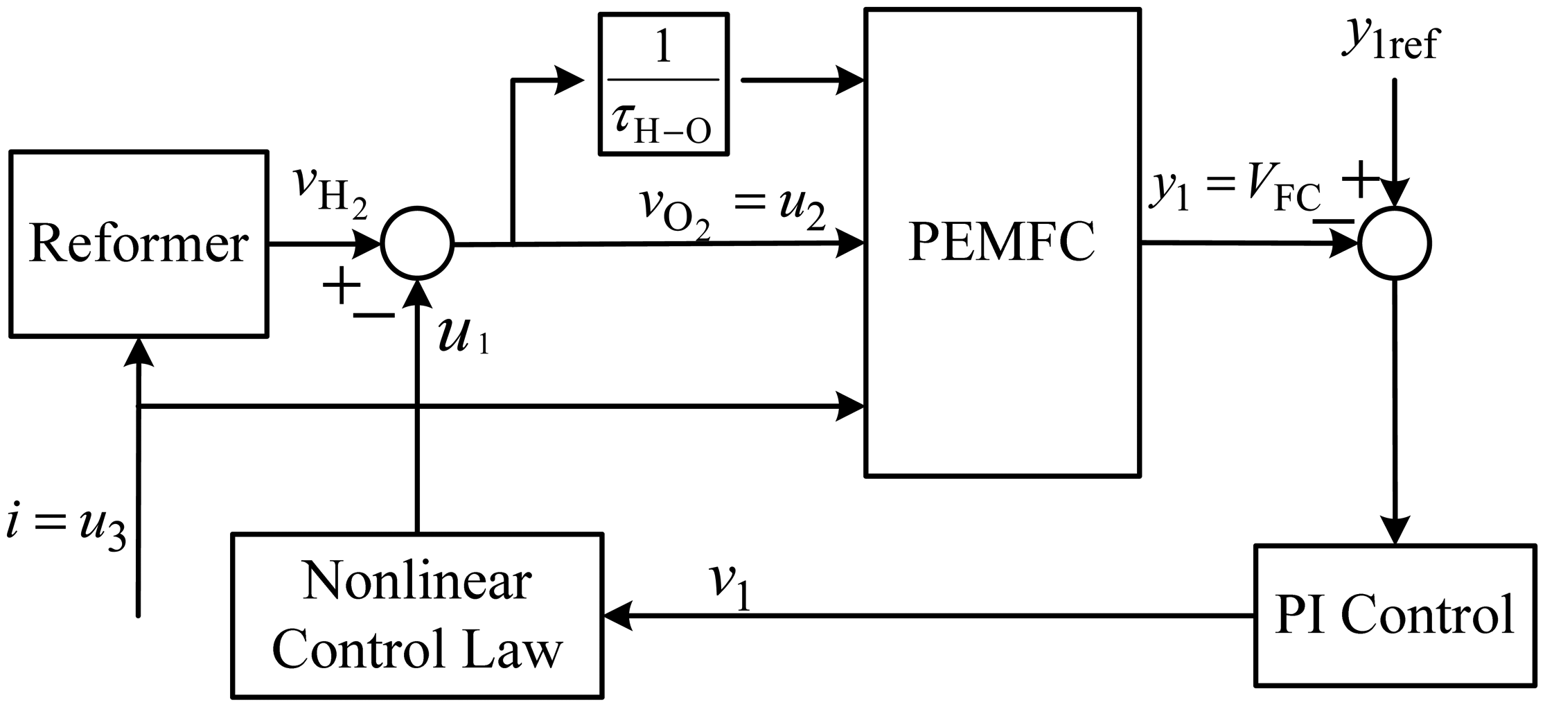
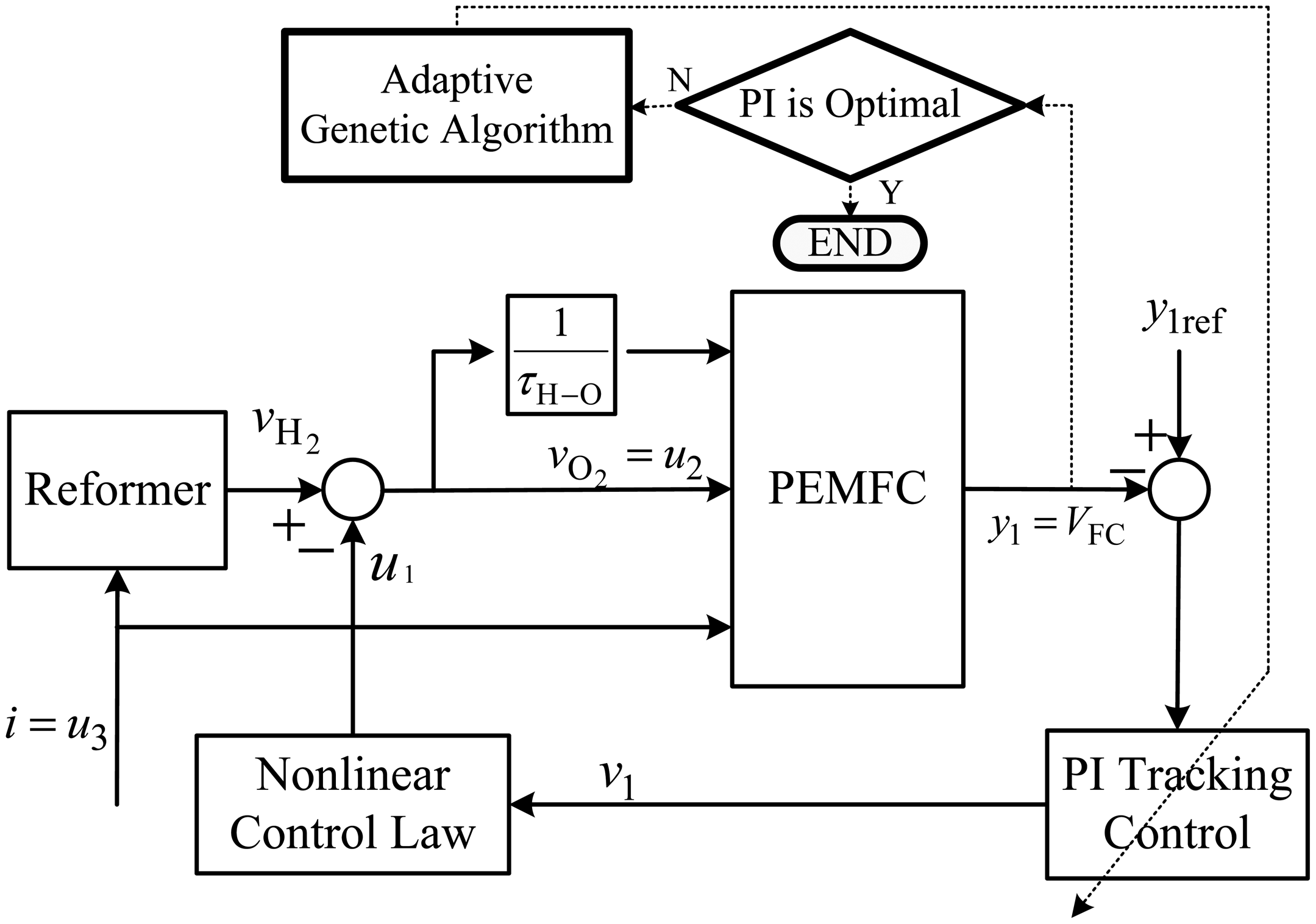
As derived in the preceding section, an original nonlinear system is converted into a linear and input-output decoupling system. Besides, the control performance can be improved by the addition of a PI controller into a feedback control law u₁. The control law u₁ mostly adjusts the inlet flow rate of hydrogen from the reformer, while the oxygen flow rate is dependent on the flow ratio τ_H–O between hydrogen and oxygen [20]. Figure 1 is a block diagram of the proposed PEMFC nonlinear control with linearization and input-output decoupling. Appropriate amounts of the hydrogen and oxygen at the cell inlets are supplied to a PEMFC according to the load changes.

4. Optimal PI Tracking Control Design Using an Adaptive Genetic Algorithm

Proven more efficient than conventional algorithms, genetic algorithms were developed as a random search approach to locate the global optimum. However, in consideration of the distinct nature of search problems, a simple GA is not expected to find the global optimum as intended [21]. In an effort to handle a local convergence problem, an adaptive genetic algorithm (AGA), a prior work described in [22], is adopted to design the parameters of PI tracking control. The brief block diagram of AGA used to the search of the optimal parameters for the PI tracking control of the input-output decoupling linearization controller is illustrated in Figure 2.

5. Simulation Results and Discussion

To demonstrate the performance of the proposed nonlinear control law, a Matlab/Simulink is used to build the PEMFC system dynamic model with nonlinear controller. In this work, the simulation parameters adopted are those of a single Ballard Mark V PEMFC. Hydrogen is employed as the fuel, oxygen is the oxidant, and a Nafion 117 PEM (Walther Grot of DuPont, Wilmington, DE, USA) is employed as well. All the cell parameters are tabulated in

Table 1. Parameters of the Ballard Mark V fuel cell.

Symbol	Parameters	Symbol	Parameters
T	343.15 K	ξ1	−0.948
A	50.6 cm2	ξ2	(286 + 20 ln A + 4.3 ln cH2) × 10−5
λ	178 μm	ξ3	7.6 × 10−5
PH2	1 atm	ξ4	−1.93 × 10−4
PO2	1 atm	Ψ	23
B	0.016 V	Jmax	150 mA/cm2
RC	0.0003 Ω	Jn	1.2 mA/cm2

[14].

To compare the efficiency of the proposed nonlinear controller, the conventional PID controller is also implemented for the PEMFC system. All the PID control parameters had been determined ahead of the simulation. Employing the Ziegler-Nichols rule to tune such parameters, as the first step, setting K_i = K_d = 0, increase K_p until an oscillation is produced. Then as the second step, the value of K_p is now multiplied by 0.6 to get the final K_p. In the end, all the final parameters are found as K_p = 3, K_i = 1.2 and K_d = 0.1.

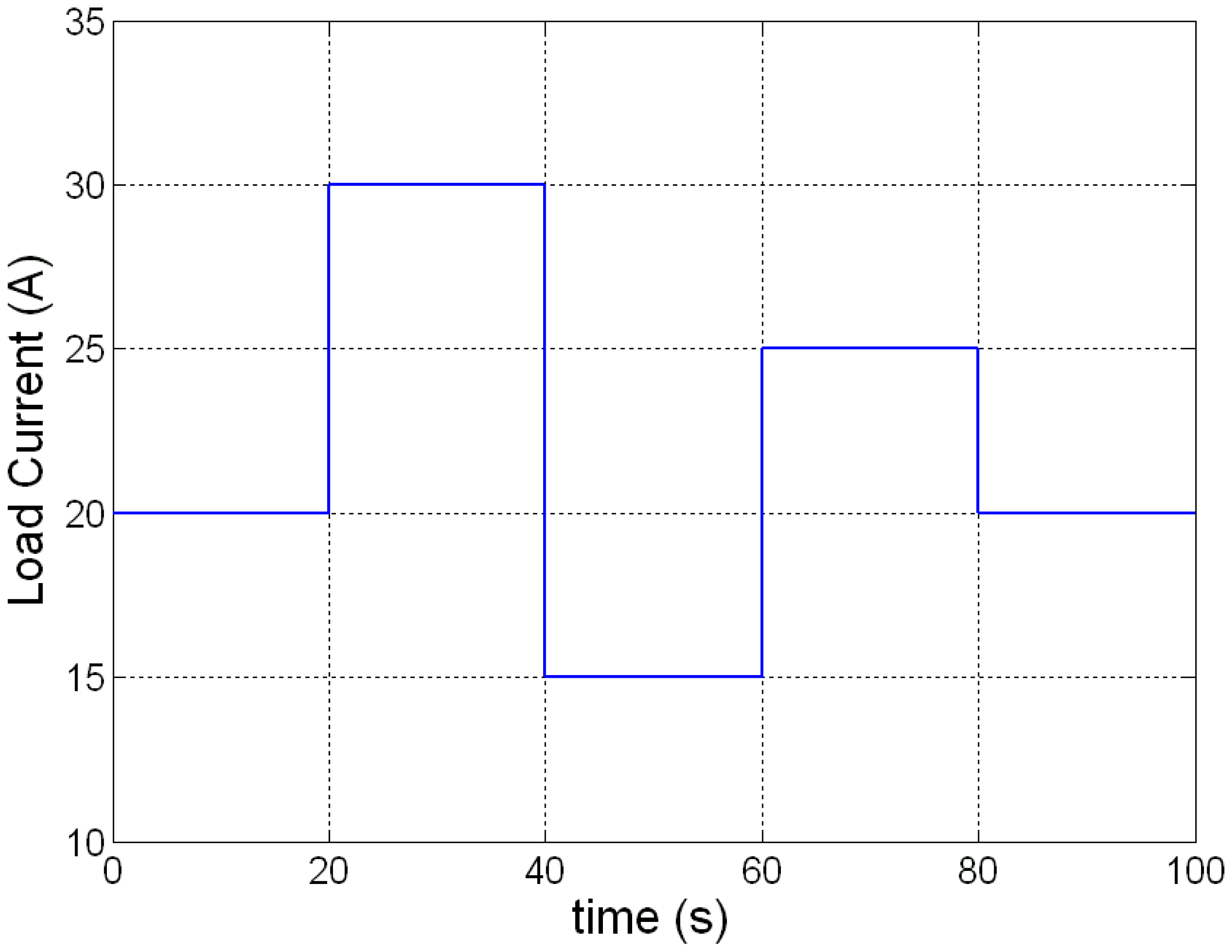
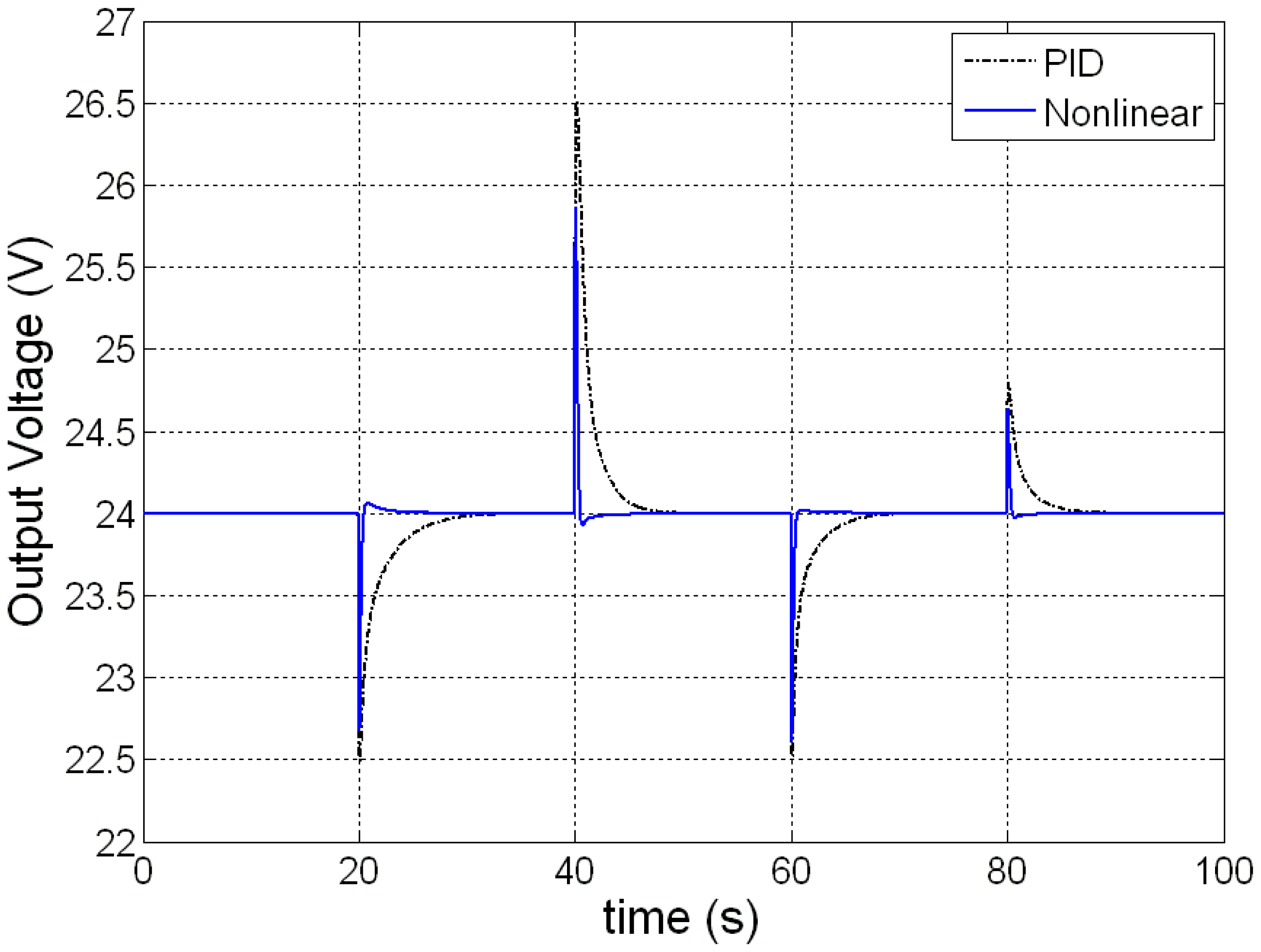
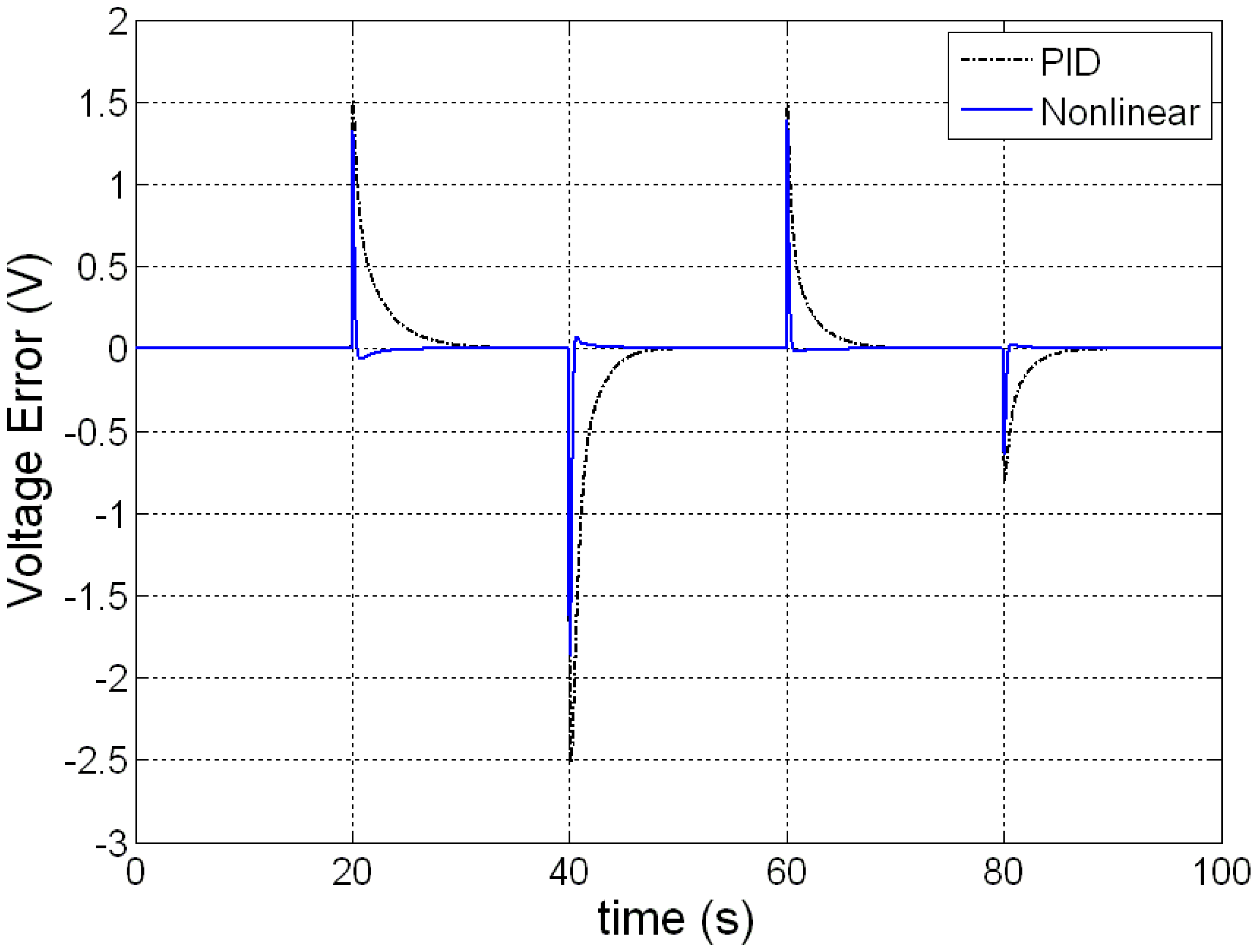
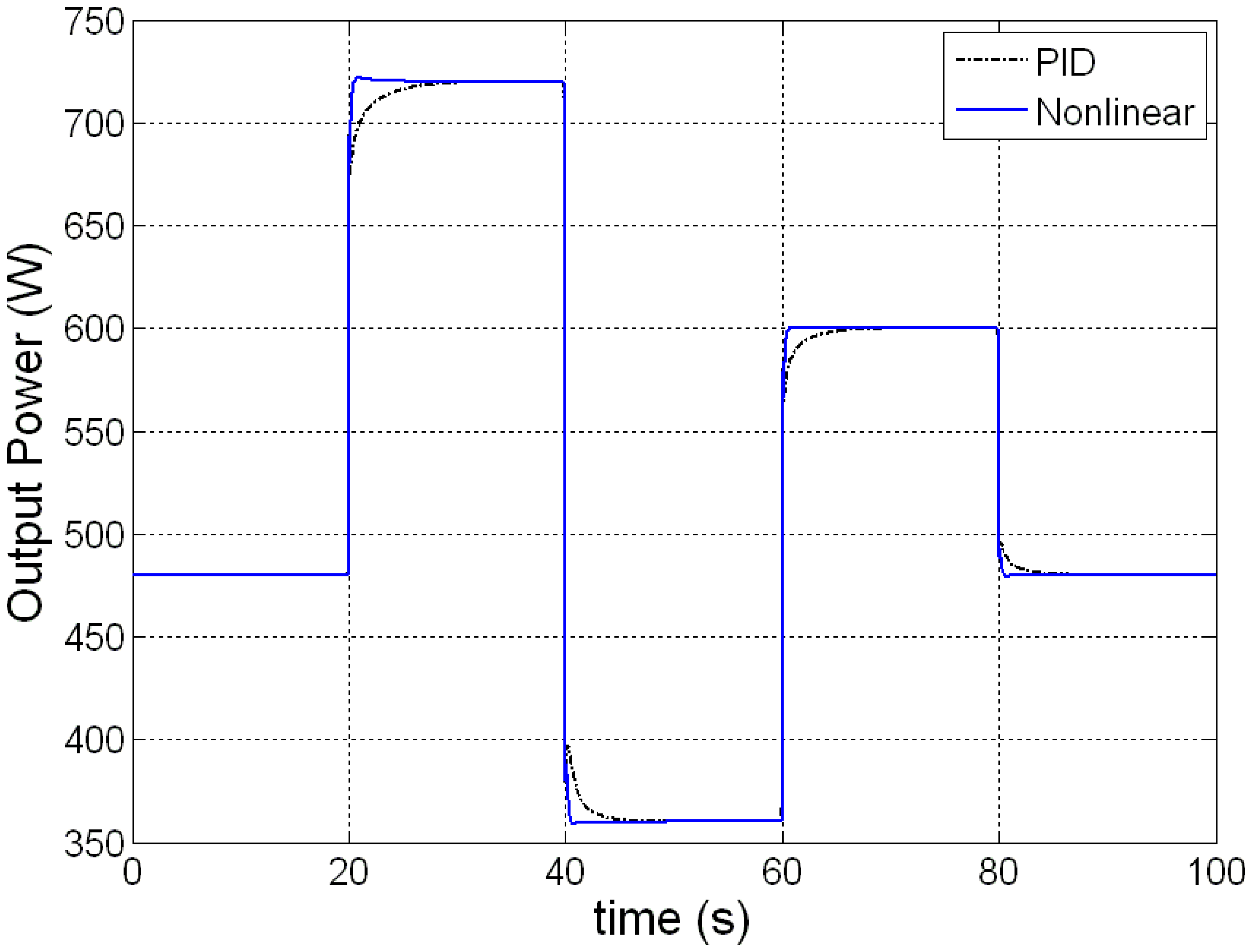
The load current is changed for testing the transient behaviors of PEMFC with nonlinear control. Figure 3 shows the variation of load current step changes from 20 to 30, 15, 25, 20 A at times t = 20, 40, 60, 80 s, respectively. The dynamic responses of the PEMFC as the load current changed in step are shown in Figures 4, 5, 6, 7, 8, 9 and 10. Figure 4 shows the variation of output voltage. It is obvious that the output voltage under nonlinear control remains in a well transient and steady-state response under the disturbances caused by the load changes. A well regulated output voltage of 24 V is seen from the simulations. Figure 5 gives the output voltage error. It is noteworthy that, the system, regulating output voltage to the target value of 24 V, exhibits a maximum error of 1.9 V by nonlinear control, which is much lower than that, i.e., 2.5 V, achieved by PID. This improvement is indeed a clear advantage of input-output feedback linearization based nonlinear control over PID control. Plotted in Figure 6 is the output power variation, which is proportional to the load current with the output voltage regulated at 24 V. From this figure, one can also observe that the FC with nonlinear control has very quick responses to the disturbances caused by the load changes.

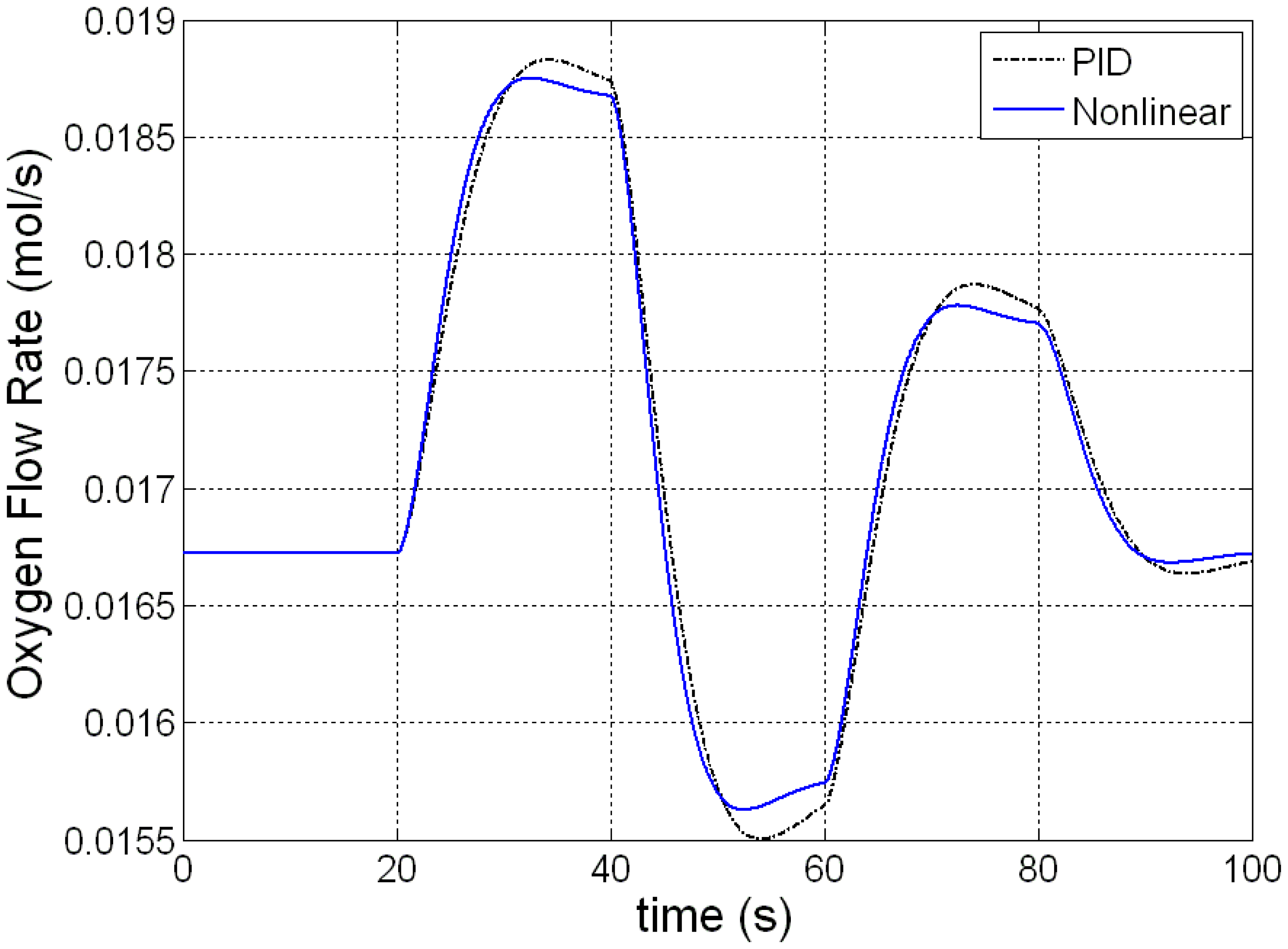
Figures 7 and 8 give the dynamic responses of the hydrogen and the oxygen flow rates under the load current variations. The hydrogen flow rate shown in Figure 7 is directly from the reformer which is adjusted by the load changes. The oxygen flow rate shown in Figure 8 has the same response as that in Figure 7, only with smaller magnitude because the oxygen flow rate is simply determined by the hydrogen–oxygen flow ratio.

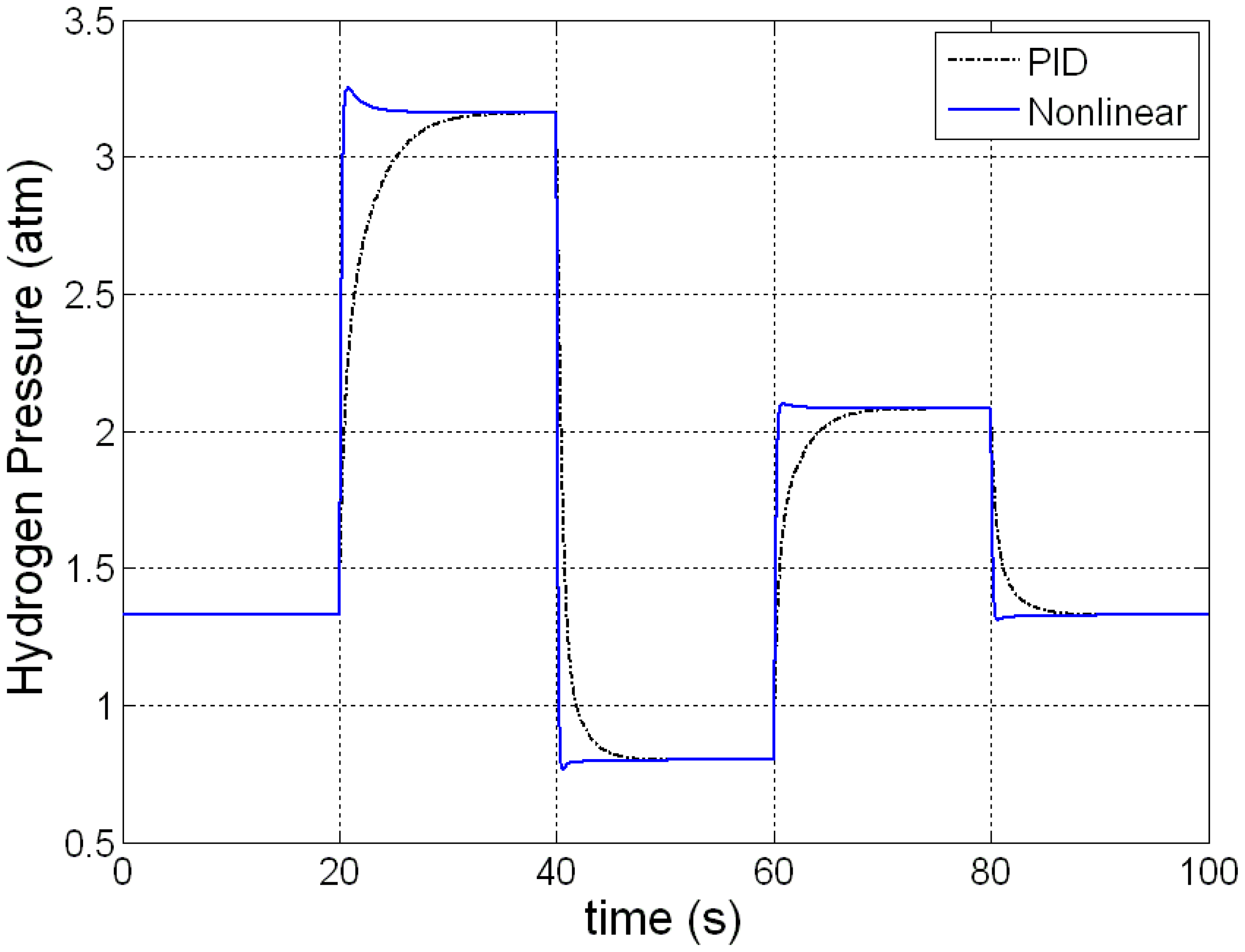
Figures 9 and 10 give the dynamic responses of the hydrogen and the oxygen pressures under the load current variations. In response to an abrupt rise in the load current from 20 A to 30 A at the instant t = 20 s on account of a sudden drop in ohmic voltage drop, the nonlinear controller speeds up the gas flow in the fuel reformer, such that the reactive gas pressures at the inlets are elevated. Consequently, such ohmic voltage drop is compensated, following which the cell stack output voltage is regulated to the target value. This accounts for the voltage drop at the instant t = 20 s. In contrast, in response to a drop in the load current at the instant t = 40 s, the cell output voltage is regulated at 24 V as before through feedback by reducing the flow rate in the fuel reformer and accordingly the pressures of the cathode/anode inlet gases respectively.

Even though a superior control performance is seen, the PI tracking controller parameters, determined by the Ziegler-Nichols rule, are not necessarily the optimal ones. For this sake, the following is devoted to the search of the optimal control parameters and the performance comparison. Tabulated in

Table 2. Parameters adopted when performing an AGA.

Parameter		Value
Searching Range	Kp	0∼100
	Ki	0∼100
Population Size		50
Generation Number		20
Bit Number		30
Crossover Rate		0.9
Mutate Rate		0.03

are searching range, population size, generation number, bit number, crossover rate and Mutate rate when performing a genetic algorithm to seek the optimal parameters.

Consequently, the optimal parameters obtained are K_up = 99.47 and K_ui = 21.11.

Plotted in Figure 11 is the output voltage comparison between an optimized input-output feedback linearization controller and a non-optimized one. Demonstrated in Figure 12 is an enlarged view of Figure 11 between t = 39.5 and 42 s, from which a shorter transient response time of 0.2 s is seen relative to the non-optimized case, before the system converges to the target value of 24 V. The results indicate the feasibility of a genetic algorithm to optimize the PEMFC control system.

6. Conclusions

A nonlinear control strategy utilizing the linearization and input-output decoupling approach is proposed in this paper for nonlinear control of PEMFCs. A MIMO dynamic nonlinear model of a PEMFC appropriate for developing the nonlinear controller is also presented. By adding a tracking controller to the state feedback control law, which is optimally designed by AGA, the steady-state errors due to parameter uncertainty can be effectively reduced. The comprehensive simulation results demonstrate that the PEMFC with nonlinear control has better transient and steady-state performance compared to conventional linear techniques. The proposed nonlinear control strategy and dynamic nonlinear model have the potential to become valuable tools for modeling and control of PEMFC systems.

References

- Yoshida, A.; Amano, Y.; Murata, N.; Ito, K.; Hasizume, T. A comparison of optimal operation of a residential fuel cell co-generation system using clustered demand patterns based on Kullback-Leibler divergence. Energies 2013, 6, 374–399. [Google Scholar]
- Zhang, N.; Gu, W.; Yu, H.J.; Liu, W. Application of coordinated SOFC and SMES robust control for stabilizing tie-line power. Energies 2013, 6, 1902–1917. [Google Scholar]
- Zhang, H.C.; Lin, G.X.; Chen, J.C. The performance analysis and multi-objective optimization of a typical alkaline fuel cell. Energy 2011, 36, 4327–4332. [Google Scholar]
- Leo, T.J.; Raso, M.A.; Navarro, E.; Mora, E. Long term performance study of a direct methanol fuel cell fed with alcohol blends. Energies 2013, 6, 282–293. [Google Scholar]
- Liu, W.S.; Chen, J.F.; Liang, T.J.; Lin, R.L. Multicascaded sources for a high-efficiency fuel-cell hybrid power system in high-voltage application. IEEE Trans. Power Electron. 2011, 26, 931–942. [Google Scholar]
- Ugartemendia, J.; Ostolaza, J.X.; Zubia, I. Operating point optimization of a hydrogen fueled hybrid solid oxide fuel cell-steam turbine (SOFC-ST) plant. Energies 2013, 6, 5046–5068. [Google Scholar]
- Almeida, P.E.M.; Simoes, M.G. Neural optimal control of PEM fuel cells with parametric CMAC networks. IEEE Trans. Ind. Appl. 2005, 41, 237–245. [Google Scholar]
- Schumacher, J.O.; Gemmar, P.; Denne, M. Control of miniature proton exchange membrane fuel cells based on fuzzy logic. J. Power Sources 2004, 129, 143–151. [Google Scholar]
- Pukrushpan, J.T.; Stefanopoulou, A.G.; Peng, H. Control of fuel cell breathing. IEEE Control Syst. Mag. 2004, 24, 30–46. [Google Scholar]
- Purkrushpan, J.T.; Peng, H. Control of Fuel Cell Power Systems: Principle, Modeling, Analysis and Feedback Design, 1st ed.; Springer-Verlag: Berlin, Germany, 2004; pp. 71–86. [Google Scholar]
- Nijmeijer, H.; van der Schaft, A.J. Nonlinear Dynamical Control Systems; Springer-Verlag: Berlin, Germany, 1990; pp. 172–198. [Google Scholar]
- Slotine, J.J.E.; Li, W. Applied Nonlinear Control; Prentice-Hall: New York, NY, USA, 1991; pp. 112–137. [Google Scholar]
- Te Braake, H.A.B.; van Can, J.; Scherpen, J.M.A.; Verbruggen, H.B. Control of nonlinear chemical processes using neural models and feedback linearization. Comput. Chem. Eng. 1998, 22, 1113–1127. [Google Scholar]
- Corrêa, J.M.; Farret, F.A.; Canha, L.N.; Simões, M.G. An electrochemical based fuel cell model suitable for electrical engineering automation approach. IEEE Trans. Ind. Electron. 2004, 51, 1103–1112. [Google Scholar]
- Pathapati, P.R.; Xue, X.; Tang, J. A new dynamic model for predicting transient phenomena in a PEM fuel cell system. Renew. Energy 2005, 30, 1–22. [Google Scholar]
- Maher, A.R. Modelling of proton exchange membrane fuel cell performance based on semi-empirical equations. Renew. Energy 2005, 30, 1587–1599. [Google Scholar]
- Chen, H.C. Mathematic modeling and characteristics analysis of a proton exchange membrane fuel cell. J. Nanoelectron. Optoelectron. 2012, 7, 132–137. [Google Scholar]
- Khan, M.J.; Iqbal, M.T. Dynamic modeling and simulation of a small wind-fuel cell hybrid energy system. Renew. Energy 2005, 30, 421–439. [Google Scholar]
- El-Sharkh, M.Y.; Rahman, A.; Alam, M.S.; Shakla, A.A.; Byrne, P.C.; Thomas, T. Analysis of active and reactive power control of a standalone PEM fuel cell power plant. IEEE Trans. Power Syst. 2004, 19, 2022–2028. [Google Scholar]
- Sharifi Asl, S.M.; Rowshanzamir, S.; Eikani, M.H. Modelling and simulation of the steady-state and dynamic behaviour of a PEM fuel cell. Energy 2010, 35, 1633–1646. [Google Scholar]
- Zbigniew, M. Genetic Algorithms + Data Structures = Evolution Programs, 3rd Revised and Extended ed.; Springer: New York, NY, USA, 2012; pp. 95–113. [Google Scholar]
- Chen, H.C. Optimum capacity determination of stand-alone hybrid generation system considering cost and reliability. Appl. Energy 2013, 103, 155–164. [Google Scholar]