1. Introduction
Extraction of wave energy became one of the most challenging technological problems of the beginning of the 21st century. This type of energy is abundant and is more predictable than wind or solar energy, although it is in general less predictable than tidal energy. Thus, despite a degree of uncertainty related to the variability in the wave climate, improvements in the accuracy of the wave evaluations in the coastal areas would enhance also the accuracy of the predictions that future energy convertors yield. Wave energy is not only more predictable than wind or solar energy but it has also a higher energetic density allowing in this way extraction of more energy in smaller areas.
Portugal has a substantial wave power potential, because of its location in relatively high latitude and a long stretch of ocean immediately to the west. Using a wave prediction system based on WAM (Wave prediction Model) [
1] for wave generation and SWAN (Simulating Waves Nearshore) [
2] coastal transformation, various computational strategies have been developed and validated for this coastal environment [
3,
4,
5] based on an extended hindcast study covering the whole North Atlantic for proper modeling of the swell conditions [
6].
Furthermore, using the same wave prediction system [
7,
8] performed evaluations to identify the most relevant patterns of the spatial distribution of the wave energy in the Portuguese continental nearshore. The same wave prediction system was focused also on the Portuguese archipelagoes, Madeira and Azores, and some significant patterns for the wave energy in these areas are presented in [
9,
10,
11]. Moreover, after its calibration the above wave prediction system based on the spectral phase averaged wave models WAM and SWAN is currently used for operational forecast and focused on the Portuguese continental nearshore, as described in [
12].
The above mentioned studies allowed not only an evaluation of the average and extreme wave conditions and energy in the Portuguese nearshore, both continental and archipelagoes, but also the identification of some hot spots. These are coastal areas where due to the bathymetric features, or to some other particularities, the wave energy is higher than in the neighboring areas and they are usually the most appropriate for the wave energy conversion. On the other hand, the previous works demonstrated also the importance of designing diagrams for the bivariate distributions of the occurrences corresponding to the sea states defined by significant wave height and energy period. Such scatter diagrams, elaborated based on long term wave model simulations, can provide fundamental information concerning the performance of various wave energy converters (WEC) operating in a specific location. In this connection, an important observation is that in the same coastal environment various technologies for wave energy extraction can have different power production capabilities.
Starting from this point, the objective of the present work is to perform evaluations of the performance of five different technologies for the wave energy extraction in the Portuguese continental nearshore, which have been chosen as some relevant ones among the various available ones [
13]. These assessments are based on medium term simulations, [
14] with a wave prediction system that uses WW3, [
15] for wave generation at the scale of the entire North Atlantic Ocean forced using reanalysis wind data of NCEP/NCAR and SWAN for the coastal wave transformation forced with wind fields produced by the atmospheric model MM5 (Fifth-Generation NCAR/Penn State Mesoscale Model, [
16]. More details related to the MM5 model implementation on the West Iberian coast are given in [
17]. The results provided by this system were evaluated against the measurements coming from the directional buoys that operate in the Portuguese nearshore. Both direct comparisons and statistical analyses show that in general it is a good concordance between the model data and the measurements.
Using the above wave modeling system, [
18] performed model simulations focused on the two Portuguese pilot areas Aguçadora in the north and São Pedro de Moel in the central part of the Portuguese continental nearshore. Two medium resolution computational domains (with the spatial resolution of 0.008°, 880 m, in both directions) were defined and their extensions in the geographical space are also indicated in
Figure 1. Simulations with the above wave prediction system were carried out for a three-year time interval January 2009–December 2011, and on this basis evaluations of the efficiency of some technologies for the wave energy extraction were performed.
Figure 1.
Distribution of the mean wave power for simulations from January 2009 to December 2011 in the two medium resolution computational domains. The positions of the reference points are also indicated; (a) northern computational domain (and the reference points denoted as the A-points); (b) central computational domain (and the reference points denoted as the B-points). The P-points represent the A and B points, respectively for which the bivariate diagrams were designed.
2. Wave Conditions and Energy in the Portuguese Continental Nearshore
Following the most relevant patterns for the spatial distribution of the wave power, corresponding to the average energetic conditions in the two medium resolution areas, fifteen points were defined in the northern computational domain and sixteen reference points were defined in the central computational domain. Their positions are indicated in
Figure 1.
They will be denoted as the A-points (in the northern area,
Figure 1a and the B-points (in the central computational domain,
Figure 1b. The background of
Figure 1 illustrates the distributions of the mean wave power in the two medium resolution computational domains corresponding to the three-year period of model simulations (January 2009–December 2011), evaluations of some wave parameters were made for all the above reference points considered.
As regards the northern computational domain, the results are presented in
Table 1 while for the central computational domain the same results are given in
Table 2. The above results are related to the entire time period of three years that will be denoted in the present work as total time.
Besides the standard wave parameters as: Hs (significant wave height), Tp (peak period) and DIR (mean wave direction), some other parameters as Pw (wave power), Te (wave energy period) and Hsw (significant swell height) are also evaluated.
Thus, in SWAN, the wave power components (expressed in W/m,
i.e., energy transport per unit length of wave front), are computed with the relationships:
where:
x,
y are the problem coordinate system (for the spherical coordinates
x axis corresponds to longitude and
y axis to latitude);
the wave energy spectrum in terms of absolute wave frequency
and wave direction
;
cx,
cy are the propagation velocities of the wave energy in the geographical space.
Table 1.
Average (and maximum) values for the main wave parameters in the reference points from the northern computational domain (A-points) as resulting from the simulations performed in the three-year period 2009–2011 (for total time).
Table 1.
Average (and maximum) values for the main wave parameters in the reference points from the northern computational domain (A-points) as resulting from the simulations performed in the three-year period 2009–2011 (for total time).
| Point | Long (°W) | Lat (°N) | Depth (m) | Hs med/Hs max (m) | Te med/Te max (s) | Tp med/Tp max (s) | Pw med/Pw max (kW/m) | DIRmed (°) | Hsw med/Hsw max (m) |
|---|
| A1 | −9.164 | 41.24 | 74 | 1.98/7.78 | 9.2/15.2 | 10.4/18.3 | 26.5/478 | 296.9 | 1.32/7.44 |
| A2 | −9.122 | 41.57 | 70 | 1.99/7.62 | 9.2/14.9 | 10.5/16.9 | 27.4/448.2 | 296.4 | 1.34/7.27 |
| A3 | −9.006 | 41.91 | 58 | 1.92/7.18 | 9.2/14.9 | 10.4/18.4 | 26.2/382.9 | 295.3 | 1.28/6.65 |
| A4 | −9.305 | 41.94 | 102 | 2.07/7.75 | 9.1/14.8 | 10.4/18.4 | 25.1/438.9 | 297.3 | 1.38/7.29 |
| A5 | −9.089 | 41.7 | 81 | 1.95/7.04 | 9.2/14.7 | 10.4/16.9 | 25.2/360.9 | 295.8 | 1.29/6.49 |
| A6 | −9.114 | 41.41 | 84 | 1.94/7.10 | 9.2/14.6 | 10.4/18.4 | 24.6/356.3 | 295.9 | 1.28/6.60 |
| A7 | −8.956 | 41.08 | 67 | 1.91/7.11 | 9.2/14.9 | 10.4/16.9 | 24.9/375.8 | 295.3 | 1.26/6.64 |
| A8 | −8.923 | 41.34 | 72 | 1.86/6.64 | 9.1/14.4 | 10.3/16.9 | 22.8/315.5 | 294.4 | 1.21/6.15 |
| A9 | −8.940 | 41.5 | 64 | 1.87/6.96 | 9.1/14.7 | 10.3/16.9 | 23.7/354.1 | 293.3 | 1.22/6.48 |
| A10 | −9.205 | 41.62 | 97 | 1.97/7.18 | 9.1/14.6 | 10.4/16.9 | 25.2/356.8 | 296.4 | 1.30/6.63 |
| A11 | −8.915 | 41.78 | 20 | 1.77/6.89 | 9.2/14.9 | 10.5/18.4 | 22.9/316.1 | 293.0 | 1.19/6.49 |
| A12 | −8.741 | 41.2 | 18 | 1.54/6.37 | 9.1/15.2 | 10.4/18.4 | 17.1/269.1 | 282.3 | 1.02/6.07 |
| A13 | −8.915 | 41.98 | 13 | 1.56/5.66 | 9.4/15.6 | 10.7/18.4 | 17.3/191.5 | 276.4 | 1.11/5.41 |
| A14 | −8.815 | 41.45 | 20 | 1.55/6.26 | 9.1/15.1 | 10.4/18.4 | 17.9/267.8 | 283.9 | 1.03/5.93 |
| A15 | −8.898 | 41.67 | 19 | 1.66/6.58 | 9.1/15.2 | 10.4/18.4 | 19.8/288.1 | 284.4 | 1.10/6.22 |
Table 2.
Average (and maximum) values for the main wave parameters in the reference points from the central computational domain (B-points) as resulting from the simulations performed in the three-year period 2009–2011 (for total time).
Table 2.
Average (and maximum) values for the main wave parameters in the reference points from the central computational domain (B-points) as resulting from the simulations performed in the three-year period 2009–2011 (for total time).
| Point | Long (°W) | Lat (°N) | Depth (m) | Hs med/Hs max (m) | Te med/Te max (s) | Tp med/Tp max (s) | Pw med/Pw max (kW/m) | DIRmed (°) | Hsw med/Hsw max (m) |
|---|
| B1 | −9.222 | 39.54 | 57 | 1.93/7.86 | 9.0/15.1 | 10.4/16.9 | 24.8/466.6 | 300.5 | 1.26/7.40 |
| B2 | −9.247 | 39.6 | 99 | 1.98/7.65 | 9.1/14.8 | 10.4/16.9 | 24.5/396.9 | 300.8 | 1.29/7.09 |
| B3 | −9.114 | 39.81 | 57 | 1.87/7.18 | 9.0/14.9 | 10.4/18.4 | 23.4/379.2 | 299.7 | 1.20/6.62 |
| B4 | −9.147 | 39.95 | 80 | 1.94/7.49 | 9.0/14.9 | 10.4/18.4 | 24.7/436.2 | 300.7 | 1.27/7.00 |
| B5 | −9.222 | 39.75 | 98 | 1.93/7.55 | 9.0/14.7 | 10.4/16.9 | 23.5/393.4 | 299.9 | 1.25/6.97 |
| B6 | −9.272 | 39.84 | 101 | 1.95/7.86 | 9.0/15.1 | 10.4/18.4 | 24.1/430.8 | 300.6 | 1.27/7.26 |
| B7 | −9.247 | 39.9 | 94 | 1.93/7.34 | 8.9/14.6 | 10.4/16.9 | 23.2/372.8 | 300.5 | 1.25/6.70 |
| B8 | −9.247 | 39.66 | 93 | 1.97/7.95 | 9.1/15.2 | 10.4/18.4 | 24.9/434.5 | 299.2 | 1.29/7.41 |
| B9 | −9.363 | 39.62 | 63 | 1.98/7.79 | 9.0/15.1 | 10.4/18.4 | 23.3/428.1 | 298.9 | 1.28/7.24 |
| B10 | −9.405 | 39.54 | 121 | 1.97/7.62 | 8.9/14.7 | 10.4/16.9 | 23.4/384.9 | 300.6 | 1.27/6.96 |
| B11 | −9.147 | 39.87 | 65 | 1.93/7.59 | 9.1/14.9 | 10.4/18.4 | 24.9/420.2 | 300.2 | 1.26/7.04 |
| B12 | −9.114 | 39.62 | 17 | 1.87/7.71 | 9.2/15.7 | 10.6/18.4 | 24.8/369.1 | 293.8 | 1.29/7.42 |
| B13 | −9.073 | 39.74 | 22 | 1.73/7.19 | 9.0/15.3 | 10.4/18.4 | 21.2/358.3 | 297.7 | 1.13/6.79 |
| B14 | −8.973 | 39.99 | 22 | 1.69/7.05 | 8.7/15.5 | 10.4/18.4 | 20.3/338.9 | 298.3 | 1.09/6.58 |
| B15 | −9.031 | 39.84 | 21 | 1.73/7.24 | 9.1/15.4 | 10.5/18.4 | 21.7/360.1 | 297.9 | 1.14/6.85 |
| B16 | −9.156 | 39.53 | 23 | 1.84/7.93 | 9.3/15.4 | 10.6/16.9 | 24.8/427.1 | 306.5 | 1.26/7.57 |
The absolute value of the wave power is:
The wave energy period,
Te, is defined as:
The significant wave height associated with the low frequency part of the spectrum
Hsw is defined as:
in which,
ωsw represents the swell frequency (defined as
ωsw = 2
πfsw with
fsw = 0.1 Hz).
The results from
Table 1 and
Table 2 show that the maximum value for the wave power corresponding to one meter of wave front (of 478 kW/m) occurred in the northern computational domain in the reference point A1. A value of about 7.8 m for the significant wave height corresponded to this power. For the central computational domain the maximum value for the specific wave power (of 467 kW/m) occurred in the reference point B1 and the corresponding
Hs value is 7.9 m.
Since in winter time the wave climate is more consistent than in summer time, the conditions for the winter time were analyzed separately and the corresponding results (for the three-year time interval) are presented in
Table 3 for the northern computational domain and in
Table 4 for the central computational domain, respectively. Here, winter time represents the entire six-month period from October to March.
Table 3.
Average values for the main wave parameters in the reference points from the northern computational domain (A-points) as resulting from the simulations performed in the three-year period 2009–2011 (only for winter time).
Table 3.
Average values for the main wave parameters in the reference points from the northern computational domain (A-points) as resulting from the simulations performed in the three-year period 2009–2011 (only for winter time).
| Point | Hs med (m) | Te med (s) | Tp med (s) | Pw med (kW/m) | DIRmed (°) | Hsw med (m) |
|---|
| A1 | 2.43 | 10.1 | 11.4 | 41.3 | 291.1 | 1.84 |
| A2 | 2.45 | 10.1 | 11.4 | 42.7 | 290.8 | 1.87 |
| A3 | 2.36 | 10.1 | 11.4 | 40.7 | 290.1 | 1.78 |
| A4 | 2.54 | 10.0 | 11.4 | 41.1 | 291.9 | 1.93 |
| A5 | 2.38 | 10.1 | 11.3 | 38.9 | 290.2 | 1.79 |
| A6 | 2.37 | 10.0 | 11.3 | 37.9 | 290.0 | 1.78 |
| A7 | 2.34 | 10.0 | 11.3 | 38.6 | 289.4 | 1.76 |
| A8 | 2.27 | 9.9 | 11.2 | 34.9 | 288.3 | 1.68 |
| A9 | 2.28 | 10.0 | 11.3 | 36.5 | 286.9 | 1.69 |
| A10 | 2.41 | 10.0 | 11.3 | 38.9 | 290.6 | 1.81 |
| A11 | 2.18 | 10.2 | 11.5 | 35.4 | 288.3 | 1.68 |
| A12 | 1.91 | 10.1 | 11.4 | 26.6 | 276.5 | 1.45 |
| A13 | 1.95 | 10.5 | 11.6 | 26.8 | 273.2 | 1.56 |
| A14 | 1.92 | 10.1 | 11.4 | 27.9 | 278.5 | 1.46 |
| A15 | 2.04 | 10.1 | 11.4 | 30.5 | 278.3 | 1.55 |
Table 4.
Average values for the main wave parameters in the reference points from the central computational domain (B-points) as resulting from the simulations performed in the three-year period 2009–2011 (only for winter time).
Table 4.
Average values for the main wave parameters in the reference points from the central computational domain (B-points) as resulting from the simulations performed in the three-year period 2009–2011 (only for winter time).
| Point | Hs med (m) | Te med (s) | Tp med (s) | Pw med (kW/m) | DIRmed (°) | Hsw med (m) |
|---|
| B1 | 2.38 | 9.9 | 11.4 | 38.5 | 294.5 | 1.76 |
| B2 | 2.44 | 9.9 | 11.4 | 37.8 | 295.3 | 1.81 |
| B3 | 2.29 | 9.9 | 11.3 | 36.3 | 293.4 | 1.68 |
| B4 | 2.38 | 9.9 | 11.4 | 38.4 | 294.6 | 1.77 |
| B5 | 2.37 | 9.9 | 11.3 | 36.4 | 293.7 | 1.75 |
| B6 | 2.40 | 9.9 | 11.4 | 37.5 | 294.6 | 1.79 |
| B7 | 2.36 | 9.9 | 11.3 | 35.9 | 294.3 | 1.74 |
| B8 | 2.44 | 9.9 | 11.4 | 38.9 | 292.6 | 1.82 |
| B9 | 2.42 | 9.9 | 11.4 | 39.1 | 293.3 | 1.79 |
| B10 | 2.42 | 9.8 | 11.3 | 36.1 | 294.6 | 1.78 |
| B11 | 2.37 | 9.9 | 11.4 | 38.9 | 293.9 | 1.76 |
| B12 | 2.34 | 10.3 | 11.7 | 38.9 | 287.4 | 1.84 |
| B13 | 2.12 | 9.9 | 11.5 | 32.8 | 292.3 | 1.59 |
| B14 | 2.08 | 9.9 | 11.4 | 31.5 | 292.5 | 1.56 |
| B15 | 2.13 | 10.1 | 11.5 | 33.7 | 292.8 | 1.62 |
| B16 | 2.27 | 10.2 | 11.6 | 38.5 | 303.8 | 1.77 |
As regards the average values for the total time, the maximum wave power (of 27.4 kW/m) occurs in the point A2, while average values greater than 25 kW/m occur in several other reference points from the northern computational domain (A1, A3, A4, A5 and A10). These values of the wave power correspond to significant wave heights between 1.9 m and 2 m. For the winter time, the maximum average values of the wave power (slightly over 40 kW/m) occur in the points A1, A2, A3 and A4 from the northern computational domain. In the central computational domain values over 38 kW/m for the wave power occur in the points B1, B4, B8, B9, B11, B12 and B16. These values of the winter time wave power correspond to significant wave heights between 2.3m and 2.5m.
3. Conversion of the Wave Energy into Electric Energy
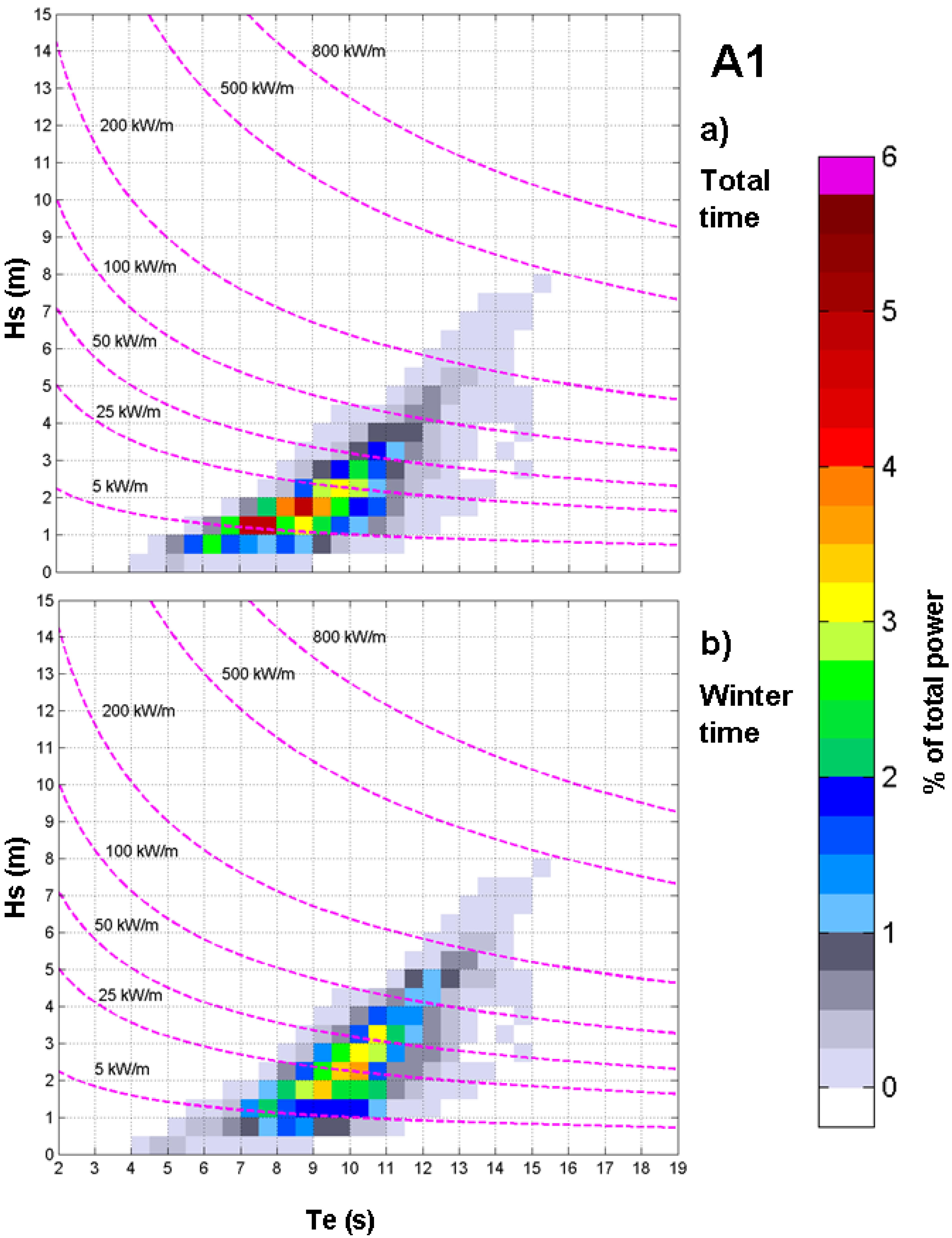
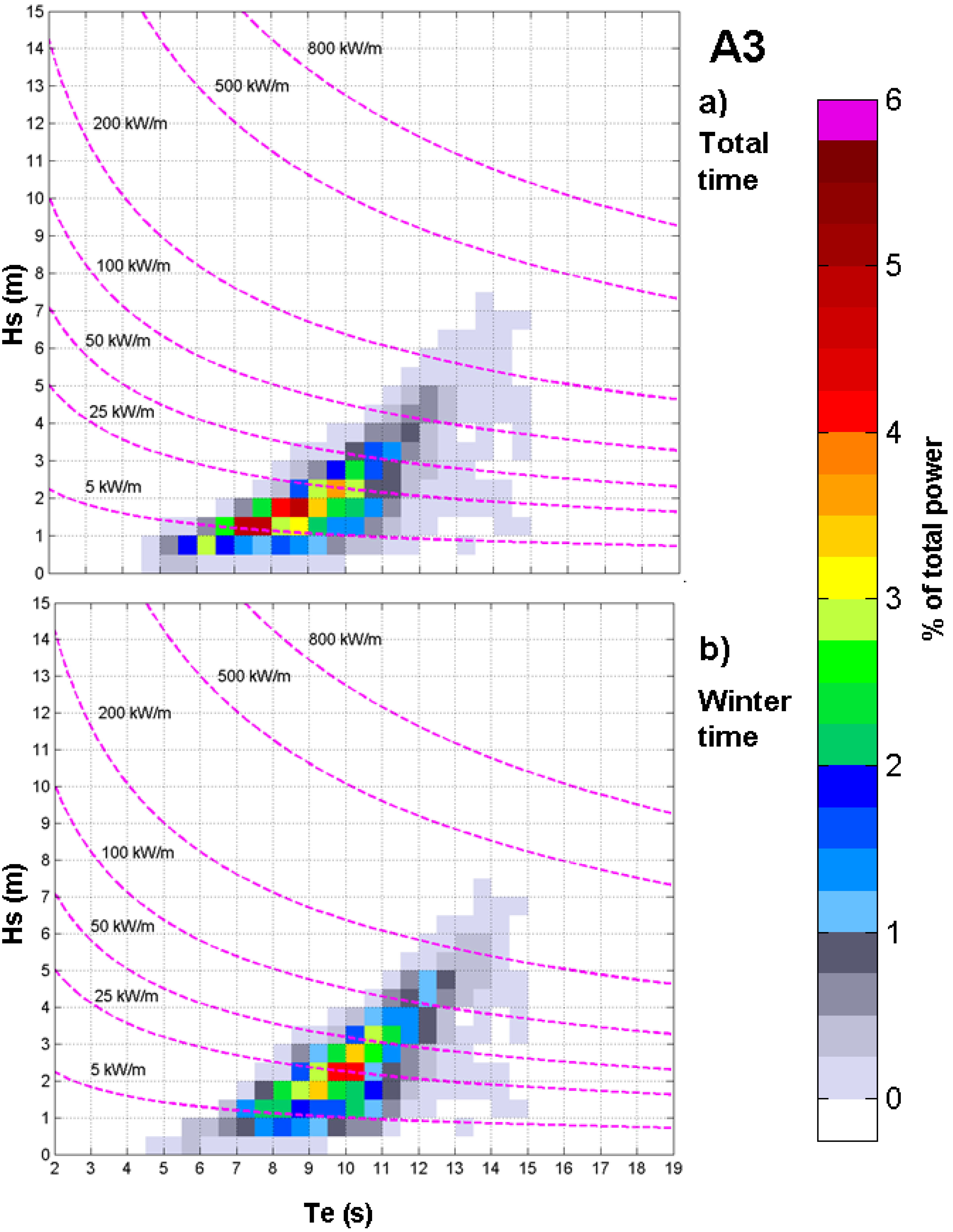
In order to make a more detailed evaluation of the energetic potential associated with the northern and central parts of the Portuguese nearshore, scatter diagrams of the Hs-Te joint distributions (and alternatively also scatter diagrams of Hs-Tp) were generated using the three-hour consecutive significant wave height and wave period time sequences resulted from the simulations with the SWAN model for the entire time interval (2009–2011) and also separately only for the winter time period, respectively. These bivariate distributions were designed for all the reference points (A-points and B-points, respectively). Such a diagram presents the probabilities of occurrences of different sea states expressed in percentages from the total number of occurrences. The sea states were structured into bins of 0.5 s × 0.5 m (ΔTe × ΔHs) and the color of each bin represents the percentage according to a color-map, which was designed the same for all diagrams and is illustrated in the color-bar of the figures.
The wave power isolines are also represented in each diagram. These have been computed using the equation of the deep water energy flux, [
19]:
where
is the energy flux in watts per meter of crest length;
ρ = 1025 kg/m
3 is the density of sea water;
g is the acceleration of gravity.
Figure 2,
Figure 3,
Figure 4 and
Figure 5 illustrate for some reference points such scatter (or bivariate) diagrams corresponding to total and winter time respectively. In order to provide a better picture of these diagrams, for each computational domain the results in two reference points are presented.
Figure 2 reflects the wave conditions from the reference point A1, which is located in relatively deep water (74 m) in the south of the northern computational domain. As the diagram presented in
Figure 2a shows, for the total time most of the occurrences in terms of significant wave height are in the interval 1–2 m while as regards the energy periods, the interval 7–10 s appears to be dominant. The winter time conditions are illustrated in
Figure 2b, where it can be seen that while the interval of the most probable wave energy periods remains almost the same, the higher percentages for the significant wave heights are moved in the interval 2–3 m.
Figure 3 is associated with the wave conditions from the reference point A3, which is located in intermediate water depth (58 m) in the north of the northern computational domain. The diagrams from
Figure 3 show rather similar features with those presented in
Figure 2 with the observation that a higher concentration of waves occur in winter time in the interval 2–2.5 m.
Figure 2.
Reference point A1 (P5 offshore); bivariate distributions of occurrences corresponding to the sea states defined by Hs and Te for the three-year time interval 2009–2011. The color scale is used to represent the contribution of the sea state to the total incident energy, as a percentage. The wave power isolines are also represented. (a) Total time; (b) Winter time.
Figure 3.
Reference point A3 (P1 offshore); bivariate distributions of occurrences corresponding to the sea states defined by Hs and Te for the three-year time interval 2009–2011. The color scale is used to represent the contribution of the sea state to the total incident energy, as a percentage. The wave power isolines are also represented. (a) Total time;(b)Winter time.
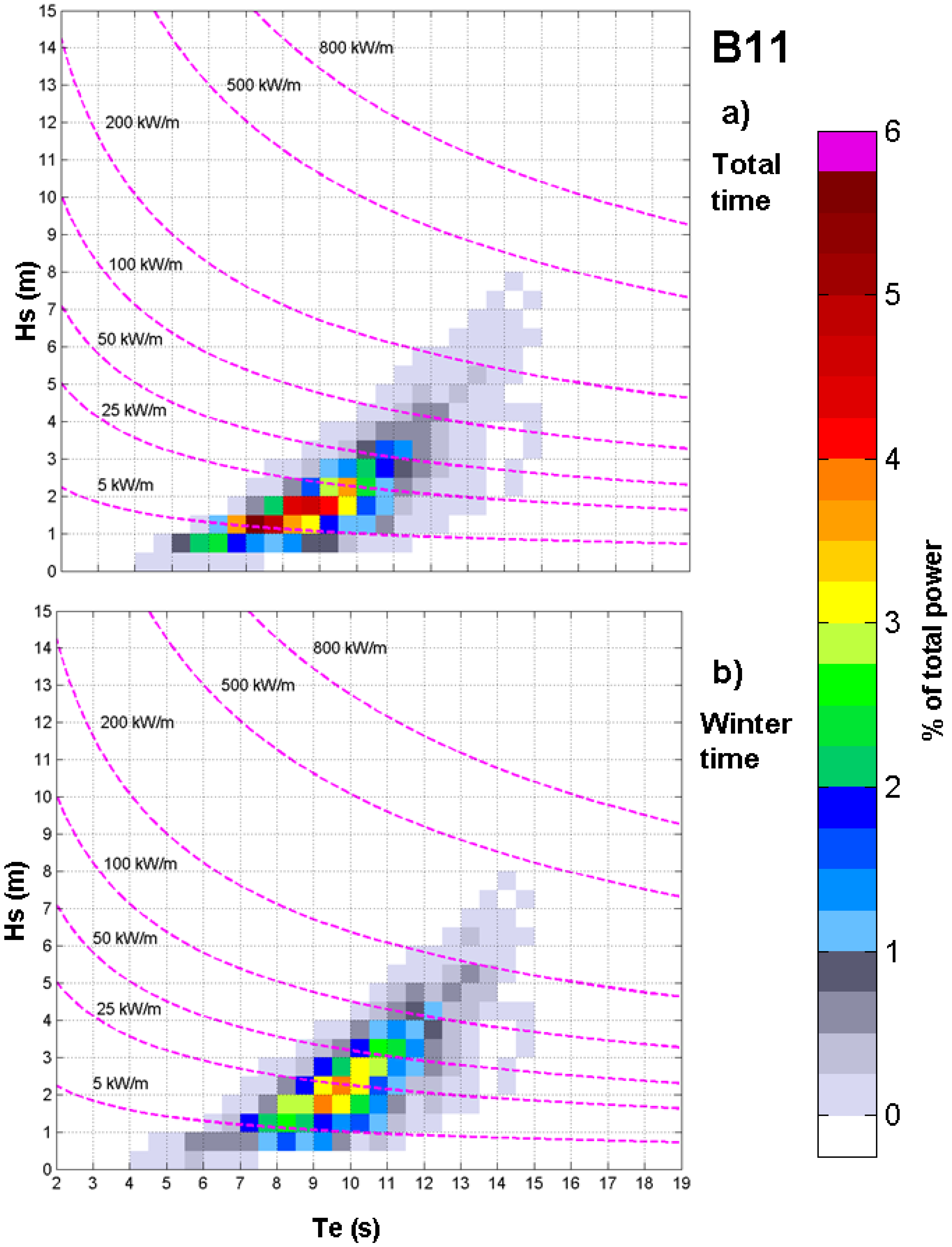
Figure 4.
Reference point B11 (P6 offshore); bivariate distributions of occurrences corresponding to the sea states defined by Hs and Te for the three-year time interval 2009–2011. The color scale is used to represent the contribution of the sea state to the total incident energy, as a percentage. The wave power isolines are also represented. (a) Total time; (b) Winter time.
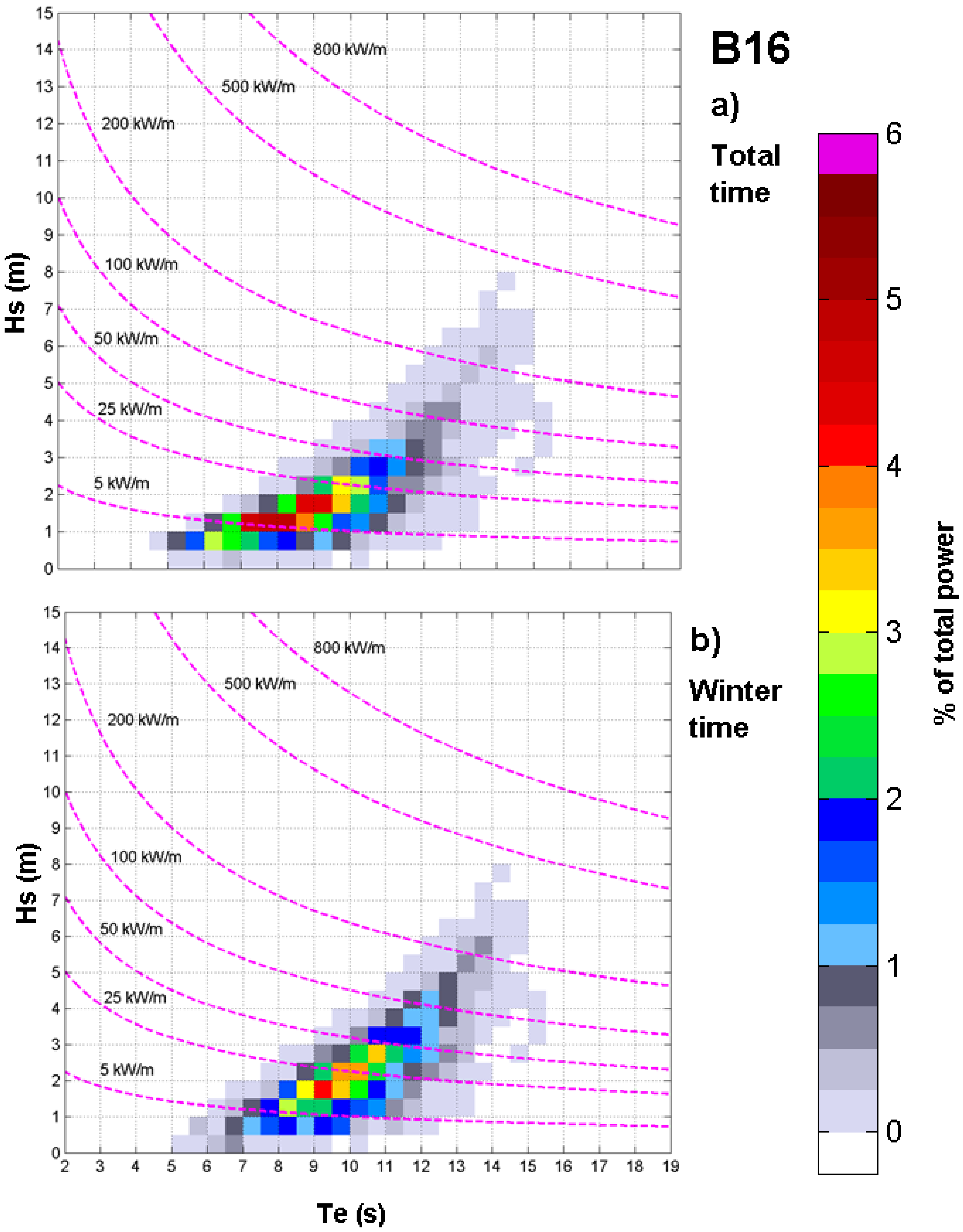
Figure 5.
Reference point B16 (P9 nearshore); bivariate distributions of occurrences corresponding to the sea states defined by Hs and Te for the three-year time interval 2009–2011. The color scale is used to represent the contribution of the sea state to the total incident energy, as a percentage. The wave power isolines are also represented. (a) Total time; (b) Winter time.
Figure 4 presents the wave conditions from the point B11 that is located also in intermediate water depth (65 m) in the northern part of the central computational domain while
Figure 5 reflects the wave climate from the point B16 that is located in relatively shallow water (23 m) in the south of the central computational domain. Although B11 is in intermediate water and B16 in shallow water the configurations of the bivariate diagrams show in general similar features. As illustrated in the figures, for the total time the concentration of the waves with significant wave heights between 1 and 2 m is even higher in the central than in the northern computational domain.
To each bivariate diagram, a table was associated, giving the wave activity during the time interval 2009–2011 for the total and winter time, respectively. The elements of these tables indicate the number of occurrences, in percentage from the total. It has to be highlighted also that the results illustrated in
Figure 2,
Figure 3,
Figure 4 and
Figure 5 are in line with those presented by [
20] that made an analysis of the wave conditions along the Galician coast which is located very close to the northern computational domain considered in the present work.
The wave model simulations give the theoretical wave power available and the characteristics of the winter time wave resources in terms of the sea states (
i.e., the characteristics of the waves providing the power), but the actual electric power yield will depend on the WEC characteristics. Because each technology has different operational ranges and also different efficiency under various sea states (some details on these issue are provided by [
21], the most appropriate WECs for a specific area are those that have the maximum efficiency in the ranges of
Hs and
Te that provide the bulk of occurrences.
WEC manufacturers provide performance data on their products as a function of Hs and of a wave period, which can be Te or any other wave period as: the peak period (Tp) or the zero crossing period (Tz), depending on the manufacturer. The performance table provides the expected power output indexed by significant wave height and wave period. A distinct pair of significant wave height and wave period is referred to as an energy bin.
Five wave energy convertors are considered in the present work. These are Aqua Buoy [
22], Pelamis [
23], Wave Dragon [
24], Oyster [
25], and SSG, Seawave Slot-Cone Generator, [
26]. From the point of view of their operability, they cover the full scale of the existent types of energy converters. Thus, Aqua Buoy and Pelamis are considered offshore devices. Wave Dragon that operates in intermediate water (usually between 25 m and 40 m) was evaluated in the present work as a nearshore converter together with Oyster (that operates at about 15 m water depth). Finally SSG is representative for a shoreline wave energy conversion system. Moreover, the devices considered cover also a wide range from the point of view of their dimensions and of their power capacities. SSG and Wave Dragon have large sizes, Oyster and Pelamis have average dimensions while Aqua Buoy is of smaller size.
The power matrices of these devices are given in the
Appendix. For the cases of Pelamis, Oyster and SSG the bins are defined in terms of
Hs and
Te and the bin resolution is 0.5 s × 0.5 m. For the cases of Aqua Buoy and Wave Dragon the bins are defined in terms
Hs and
Tp and the bin resolutions are 1 s × 0.5 m and 1 s × 1 m, respectively.
The most common way to estimate the electricity production of a WEC in a specific site is to associate to the power matrices of each WEC the matrices that give the wave activity for the respective location in a determined time interval. As the time interval considered for designing the bivariate diagrams and the tables associated to them that give the wave activity is longer, the reliability of the estimation should be better.
This approach is based on the following formula for the estimation of the average electric power that might be expected in the time interval associated with the matrix that gives the wave activity:
where
pij is the energy percentage corresponding to the bin defined by the line
i and the column
j (as given by the tables associated with the diagrams presented in
Figure 2,
Figure 3,
Figure 4 and
Figure 5); and
Pij is the electric power corresponding to the same energy bin for the WEC considered (as provided in tables given in
Appendix).
Following this approach, the results of the average electric power that is probable to be delivered by each of the five converters considered is given in
Table 5. For each computational domain the results are analysed in five reference points, denoted as P1 to P5 for the northern computational domain and as P6 to P10 for the central computational domain, respectively. Nevertheless, since the devices are designed to operate in different water depths, for each reference point two different positions were in general defined, an offshore and a nearshore position, respectively.
Table 5.
Average electric power in kW for ten reference points from north to south along the Portuguese nearshore, estimations corresponding to the characteristics of five different WEC devices.
Table 5.
Average electric power in kW for ten reference points from north to south along the Portuguese nearshore, estimations corresponding to the characteristics of five different WEC devices.
| Points | Aqua Buoy | Pelamis | Wave Dragon | Oyster | SSG |
|---|
| TT | WT | TT | WT | TT | WT | TT | WT | TT | WT |
|---|
| P1 offshore (A3) | 34.4 | 48.9 | 95.1 | 130.2 | - | - | - | - | - | - |
| P1 nearshore (A13) | - | - | - | - | 599.2 | 894.9 | 71.0 | 95.0 | 2040.3 | 3162.7 |
| P2 offshore (A4) | 31.6 | 48.2 | 86.3 | 126.7 | - | - | - | - | - | - |
| P2 nearshore (A11) | - | - | - | - | 766.7 | 1153.1 | 95.2 | 131.4 | 2676.1 | 4212.0 |
| P3 offshore (A5) | 35.7 | 50.6 | 98.0 | 133.9 | - | - | - | - | - | - |
| P3 nearshore (A15) | - | - | - | - | 729.1 | 1088.2 | 86.3 | 115.0 | 2461.9 | 3803.5 |
| P4 offshore (A2) | 36.3 | 51.4 | 101.1 | 138.8 | - | - | - | - | - | - |
| P4 nearshore (A14) | - | - | - | - | 639.7 | 964.0 | 73.2 | 97.7 | 2160.5 | 3356.6 |
| P5 offshore (A1) | 36.1 | 51.4 | 100.2 | 138.0 | - | - | - | - | - | - |
| P5 nearshore (A12) | - | - | - | - | 617.6 | 927.5 | 71.8 | 96.2 | 2089.1 | 3245.7 |
| P6 offshore (B11) | 34.1 | 48.6 | 95.8 | 131.9 | - | - | - | - | - | - |
| P6 nearshore (B15) | - | - | - | - | 780.6 | 1160.0 | 93.9 | 126.1 | 2621.3 | 4066.3 |
| P7 offshore (B3) | 32.0 | 45.4 | 90.0 | 123.1 | - | - | - | - | - | - |
| P7 nearshore (B13) | - | - | - | - | 762.6 | 1129.0 | 91.7 | 122.7 | 2560.9 | 3957.7 |
| P8 offshore (B8) | 30.4 | 44.2 | 85.7 | 121.2 | - | - | - | - | - | - |
| P8 nearshore (B12) | - | - | - | - | 859.2 | 1317.3 | 100.6 | 140.1 | 2983.3 | 4773.3 |
| P9 offshore (B2) | 36.2 | 51.8 | 102.3 | 141.7 | - | - | - | - | - | - |
| P9 nearshore (B16) | - | - | - | - | 820.8 | 1231.7 | 99.4 | 136.4 | 2846.7 | 4480.5 |
| P10 (B1) | 33.9 | 48.3 | 97.5 | 136.0 | 905.2 | 1353.6 | 107.3 | 145.1 | 3025.3 | 4710.0 |
The offshore position was considered for the converters Aqua Buoy and Pelamis while the nearshore position for the devices Wave Dragon, Oyster and SSG. At this point it has to be highlighted that although SSG is a shoreline device, the nearshore conditions were considered also for it mainly due to the limitations of the wave prediction system considered, which due to the bathymetric resolution cannot provide reliable results in shallow water.
The positions of the reference points considered are shown in
Figure 1. As mentioned, each P-point corresponds to two different reference points (one offshore and the other nearshore), the only exception being the last point (P10) that corresponds only to the point B1 located in relatively intermediate water depth (57 m). The correspondence between the P-points and the A and B points, respectively is indicated also in the first column of
Table 5, where the first point from the brackets represents the offshore position while the second indicates the nearshore position.
4. Discussion
As expected, the results presented in
Table 5 show that the winter time provides higher estimations for the average electric power than the total time. In relation to the values of electric energy expected to be delivered by each device, it can be noticed that for Aqua Buoy in total time the location P4 (corresponding to the point A2 at 70 m depth) appears to provide more electric power (36.3 kW). This value corresponds to a value of 27.4 kW/m for the wave power. In winter time the maximum expected electric power provided by the Aqua Buoy is 51.8 kW and correspond to the location P9 (which is the point B2 at 99 m depth). It is also interesting to notice that while in winter time the average wave power in P9 is 37.8 kW/m in P4 this is 42.7 kW/m. Despite this relatively high difference between the wave power in the two points (in the favour of P4), the expected electric power in P4 is slightly lower than in P9 (51.4 kW against 51.8 kW). For Pelamis, the maximum expected electric power occurs in P9 for both total (102.3 kW) and winter time (141.7 kW) with an average wave power in total time of only 24.5 kW/m.
Passing now to the nearshore devices, it can be observed that for the converters considered the optimal energetic distribution occurs in P10. In total time the electric power expected in this location is 905.2 kW for the Wave Dragon, 107.3 kW for Oyster and 3025.3 kW for SSG, corresponding to a wave power of 24.8 kW/m. In the winter time the corresponding electric power values are 1353.6 kW for the Wave Dragon, 145.1 kW for Oyster and 4710.0 kW for SGG, for a wave power of 38.5 kW/m. Nevertheless, the point P10 (that corresponds to B1) is not located in fact in shallow water (about 57 m) and for this reason the conditions in the next location from the point of view of the expected electric energy were also analyzed. This is P8 (equivalent to B12 at about 17 m water depth). Thus, for total time the expected electric power in P8 is 859.2 kW for the Wave Dragon, 100.6 kW for Oyster and 2983.3 kW for SGG for a wave power of 24.8 kW/m. For the winter time the corresponding values of the electric power are 1317.3 kW, 140.1 kW and 4773.3 kW, respectively, for a wave power of 38.9 kW/m.
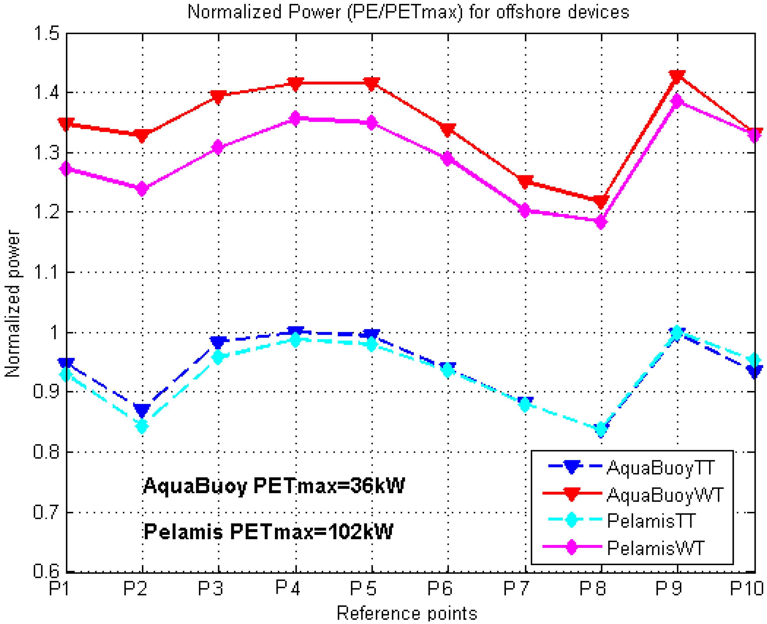
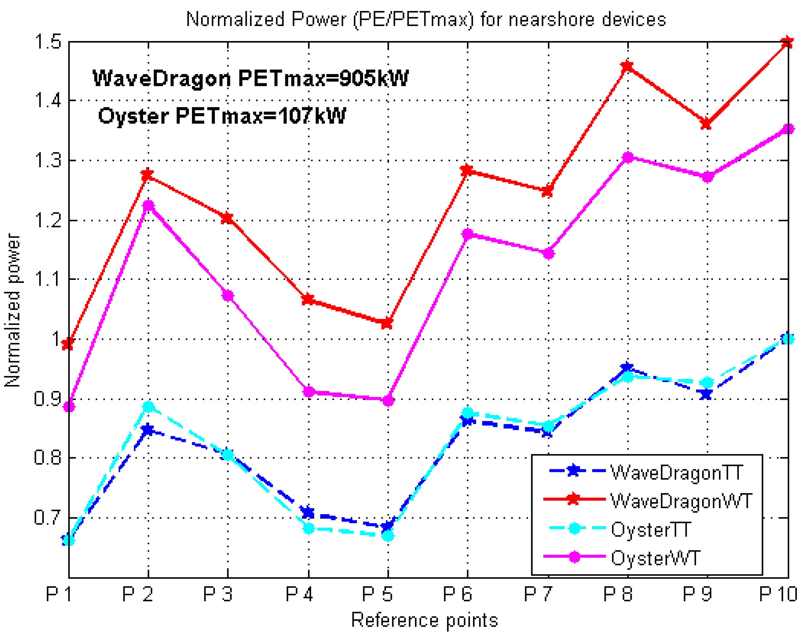
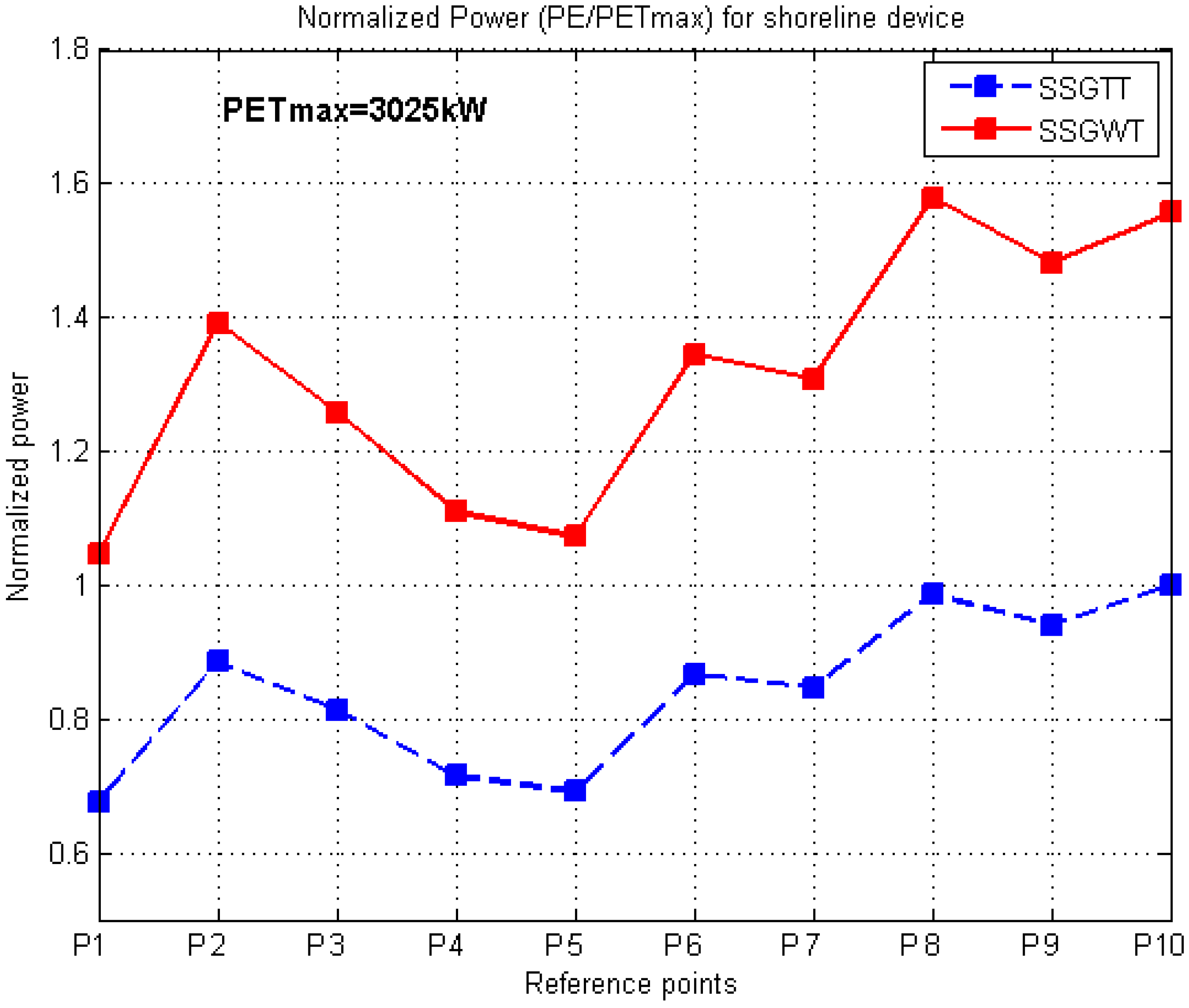
In order to provide a more comprehensive picture of the geographical variations of the electric power estimated for each wave energy converter considered, the non-dimensional normalized wave power
(PEn) was evaluated separately for each device in the ten reference points considered. Thus,
Figure 6 illustrates the normalized electric energy provided by the offshore devices (Aqua Buoy and Pelamis) in the reference points (from north to south) corresponding to total (TT) and winter time (WT), respectively. Similar representations are illustrated in
Figure 7 for the nearshore devices (Wave Dragon and Oyster) and in
Figure 8 for the SSG shoreline wave energy converter.
The normalized wave power is expressed as:
in which
PE is the estimated electric power in the respective location for the device considered; and
PET max represents the maximum value from all the geographical locations estimated for total time for the same device.
Figure 6.
Normalized electric power for the offshore devices in the reference points (from north to south) corresponding to total (TT) and winter time (WT), respectively.
Figure 6.
Normalized electric power for the offshore devices in the reference points (from north to south) corresponding to total (TT) and winter time (WT), respectively.
Figure 7.
Normalized electric power for the nearshore devices in the reference points (from north to south) corresponding to total (TT) and winter time (WT), respectively.
Figure 7.
Normalized electric power for the nearshore devices in the reference points (from north to south) corresponding to total (TT) and winter time (WT), respectively.
Figure 8.
Normalized electric power for the SSG shoreline device in the nearshore reference points (from north to south) corresponding to total (TT) and winter time (WT), respectively.
Figure 8.
Normalized electric power for the SSG shoreline device in the nearshore reference points (from north to south) corresponding to total (TT) and winter time (WT), respectively.
The above figures indicate that the relative variations of the energy power are stronger for total time than in winter time in the case of the offshore devices while for the nearshore and shoreline wave energy converters the tendency appears to be slightly opposite. In the same time, for the offshore devices the locations P2 and P8 appear to be the less energetic while the location P9 is the most energetic. For the nearshore and shoreline converters the tendency occurs again opposite since P2 and P8 appear to be now the most energetic locations, equaled only by P10 which is not in shallow water.
5. Conclusions
A medium-term evaluation of the wave conditions (corresponding to the time interval 2009–2011) was performed in the present work considering the most energetic areas from the Portuguese continental coastal environment. This was made using a wave prediction system based on spectral phase averaged models that is focused on the Portuguese continental coastal environment. The computational strategy considered is based on the WW3 model for the wave generation and on SWAN for the nearshore transformation. Two computational levels were defined for the SWAN simulations, the first covering the entire west Iberian nearshore and the second considering two medium resolution areas for the northern and the central parts of the Portuguese nearshore, respectively.
On this basis, the efficiency of five wave energy converters, covering the full scale from the point of view of their location (offshore, nearshore or shoreline), was evaluated in the Portuguese continental nearshore. The estimations were made by designing diagrams for the bivariate distributions of the occurrences corresponding to the sea states defined by significant wave height and energy period (or alternatively peak period).
The results of the present work demonstrate the importance of a correct identification of the hot energy spots but also the crucial role of a proper estimation of the wave energy distribution along the sea states reflected by the scatter diagrams. From this perspective, an important observation resulting from the present work is related to the fact that although the average value of the wave energy expected for a certain geographical location is an important indicator, only the analysis of its value can mislead in the identification of the most appropriate locations for extracting the wave energy. An example is given by the reference points denoted as P8 and P9 that correspond to the shallow water locations B12 and B16. Thus although they have about the same values for the wave power, the electric energy estimated for all the nearshore (and shoreline) devices are higher in B12. Some other relevant examples in this direction were also highlighted in the previous section related to the offshore points P4 and P9.
Finally, an important conclusion coming from the present work would be that the estimations of the expected electric power based on medium to long term wave model simulations, can provide fundamental information concerning the performance of various wave energy converters operating in a specific offshore or nearshore location. In this connection, it would be also relevant to observe that various technologies for wave energy extraction can have different efficiencies in the same coastal environment and, on the other hand, that not always the location with the highest average wave energy represents the best place for the conversion of the wave energy in electricity. In fact, sometimes other non-technical factors become determinant as discussed in [
27].


