1. Introduction
The study of energy efficiency is a highly topical subject, and the need to develop methods to improve the thermal performance of industrial systems is well recognized. Energy efficiency improvements are relevant in many fields. One of these fields is the construction industry, where energy efficiency can be improved by using appropriate materials. One type of material with interesting properties in this area is phase change materials (PCMs).
The interest in PCMs derives from their capacity to store energy as latent heat; these materials have been the focus of numerous studies [
1,
2,
3]. This energy may be used in various applications according to the demand, whether in support of air-conditioning or free-cooling [
4], walls that accumulate heat during peak hours at room temperature, then release heat in times of low temperature, heat exchanger modules [
5], or simply to modify the properties of building materials by increasing thermal inertia through the addition of a certain amount of PCM [
6,
7,
8]. Other works have researched PCMs encapsulated in different shapes in order to maximise the storage density [
9,
10], as well as improving the thermal conductivity of the PCM [
11]. Most of these works study the thermal storage of heat. Studies of thermal storage for cooling applications [
12,
13,
14] are more unusual.
Computational fluid dynamics (CFD) is a set of computer simulation techniques that help analyse and predict the performance of systems in which fluid motion plays an important role. This makes CFD an important tool that is frequently used to help design and improve products. These techniques can be applied to many fields of study, including the energy efficiency of buildings. To simulate air conditioning, works such as by Wang and Zhu [
15] studied the movement of air through various rooms and analysed the performance of fans. Tanasic [
16] studied the flow of air in an industrial building to determine the optimal placement of exhaust fans for ventilation. Transient heat transfer plays an important role in simulations in which thermal conditions are time dependent and affect the system. A Trombe wall was simulated in [
17] with special attention to the natural advection air movement to study the convection heat transfer [
18,
19]. CFD simulations can be a useful tool to analyze the evolution of systems with PCM [
20] in detail.
In this study, CFD techniques are used to simulate the thermal behaviour of a cubicle exposed to actual environmental conditions and compare it with the thermal behaviour under experimental conditions. The results of this simulation are compared with the data measured in the experimental cubicle. Thus, the ability of the simulation method to predict the thermal behaviour of the experimental construction is evaluated. Then, the cubicle is simulated under the condition of the cubicle walls containing PCM, and the results are compared with the simulation of the non-PCM-containing cubicle to study the effect of PCM on the cubicle’s thermal behaviour.
2. Experimental Setup
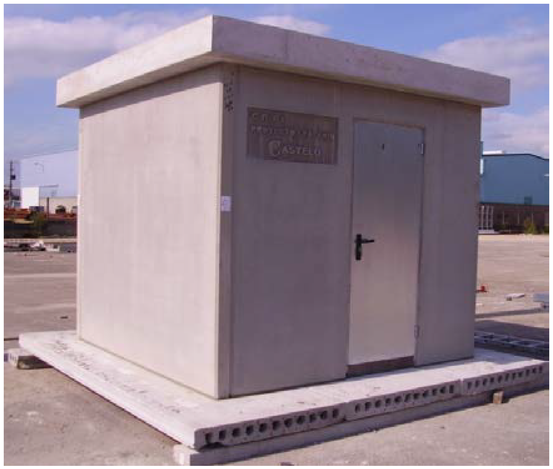
A concrete cubicle which is located in Vigo, Spain and thermal data collection system were used to study the thermal behaviour of a building in response to environmental exposure. The cubicle is made of precast, self-compacting concrete panels, which are 2.4 m high, 2.6 m wide and 12 cm thick (
Figure 1). The cubicle rests on a base made of conventional concrete; the roof was also constructed with conventional concrete and contains expanded polystyrene insulation.
Figure 1.
Experimental cubicle.
Figure 1.
Experimental cubicle.
The enclosure also contains a heat pump, which functions to maintain a constant temperature inside the cubicle. The power of the heat pump is 2500 W for refrigeration and 3400 W for heating. The control of the heat pump is regulated in order to maintain a temperature set-point of 20 °C. When a temperature sensor detects a variation of 2.5 °C higher or lower than the set-point, the cooling or heating modes are activated. Once the cooling or the heating modes are working, the system operates with an on-off regulation when the sensor detects a deviation of 1.5 °C above or below the set-point.
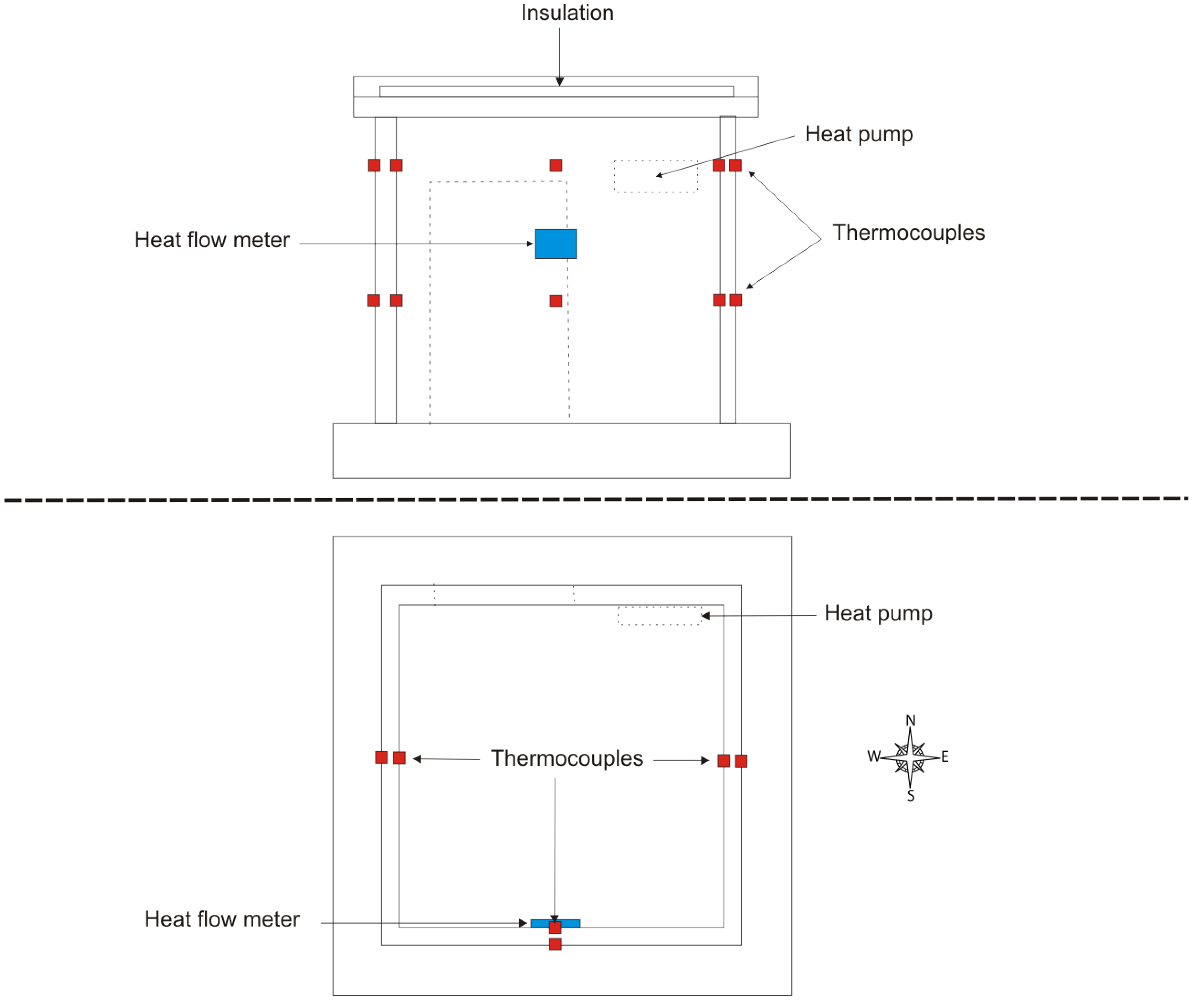
The building is equipped with a data collection system consisting of internal thermometers, thermocouples embedded at a depth of a few mm from the inner and outer surfaces of each panel (located at the horizontal centre of each panel at 1 m and 2 m above ground level) and a weather station. The thermocouples are placed on the walls facing south, east and west, as these walls experience more thermal variation due to solar radiation. The heat flow meter is placed on the inner surface of the south wall. The cubicle also has a heat pump system to study the heating or cooling of each cubicle.
Figure 2 shows a diagram comprising a front view and a top view to show the placement of these sensors and the heat pump in the cubicle.
Figure 2.
Schematic of the sensors location in the cubicle.
Figure 2.
Schematic of the sensors location in the cubicle.
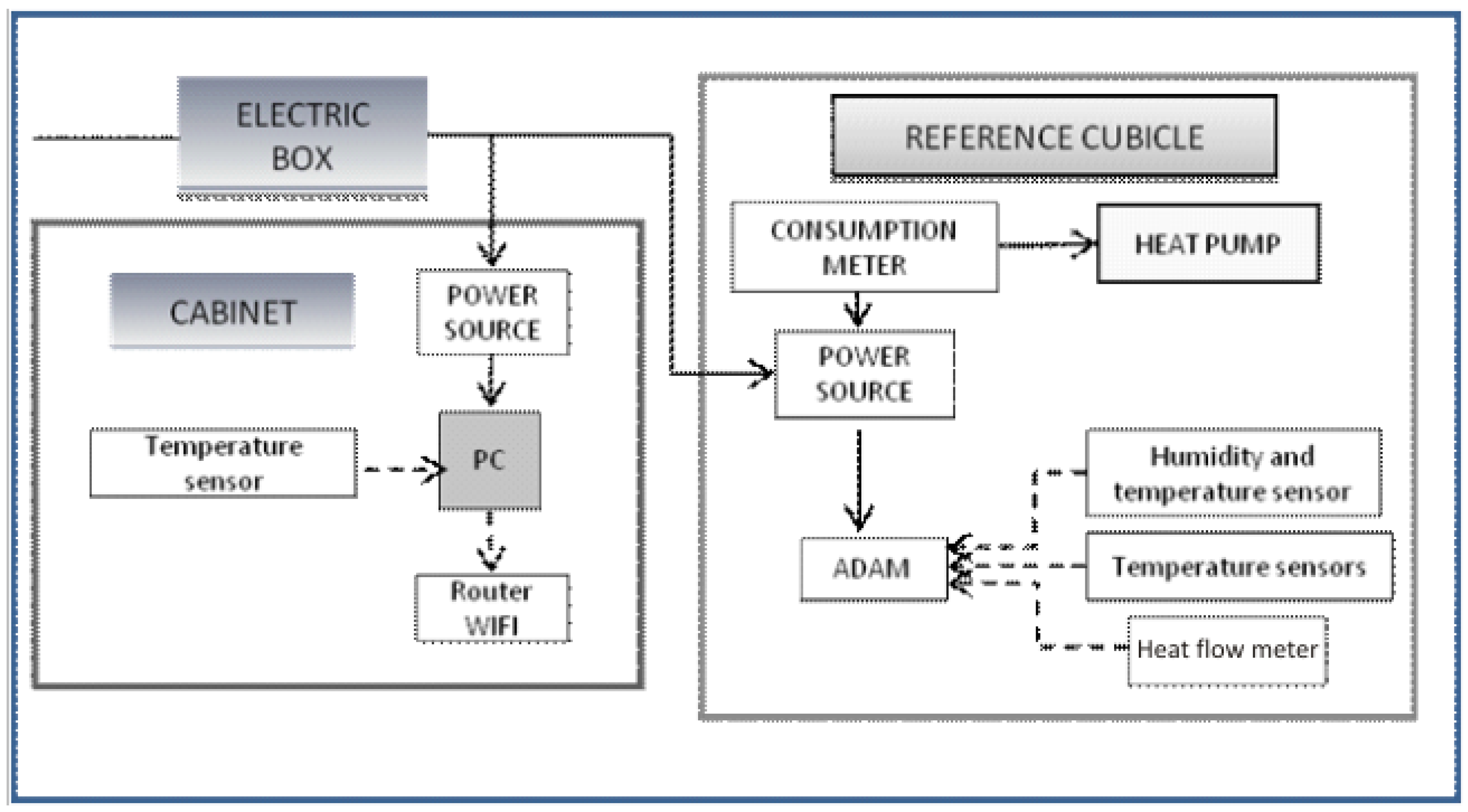
Regarding the electrical installation of the cubicle, an electrical breaker box is installed outside the cubicle to separate the electrical installation of the cubicle and the electric network. This breaker box consists of a three-phase thermal magnetic circuit breaker, an automatic differential circuit breaker and a three-phase electricity consumption meter to determine the total consumption of the cubicle installation. The consumption meter allows an evaluation of the variation in energy consumption when the heat pump operates in cooling or heating mode.
Next to the cubicle is a box with an industrial computer on which data are stored, a Wi-Fi router, a power supply unit, two 300 W sockets, a thermal magnetic circuit breaker for this portion of the installation and miscellaneous supplementary equipment.
The heat pump is installed in the door panel of the cubicle (left side entrance), along with a consumption meter, a circuit breaker, a 12 V power source, an 8-channel analog input module (model ADAM-4017 of B&B Electronics Ltd.), a humidity and temperature sensor, an electrical outlet and four temperature sensors in each of the east, south and west panels. The data acquisition program, developed for this study, allows recording of data (temperature, humidity, heat flow and consumption) at a user-selectable recording frequency.
Figure 3 shows a flow chart of the complete setup of the data acquisition system.
Figure 3.
Flow chart of the data acquisition system.
Figure 3.
Flow chart of the data acquisition system.
3. CFD Simulation
The aim of the CFD simulation presented in this paper is to reproduce the real behaviour of the system and to study other conditions without increasing the experimental investment. The methodology used for this simulation was based on modelling the geometry of the cubicle and then applying physical models that predict the system variables. Once the modelling is applied to the boundary conditions necessary for the material and thermal properties, it reproduces the real atmospheric conditions that the cubicles were subjected to during the days that were simulated. These boundary conditions include atmospheric temperature, wind speed and direction data, which were recorded by the weather station, and the calculated solar radiation during the simulated days. Ten consecutive days in October 2011 were simulated using the atmospheric data measured by the weather station, which are updated every five minutes. Solar radiation data were calculated as a function of the Sun's position with a resolution of one minute. The simulation was performed by calculating transient intervals of five minutes from October 5th to 15th, 2011, a period in which the weather was stable and sunny, which is suitable to avoid the difficulties of reproducing atmospheric variations. An unstructured, three-dimensional tetrahedral grid with approximately 1.5 × 10⁶ elements was used. The size of the grid was selected to reach high accuracy of the solutions. The size of the mesh elements is very heterogeneous and dependent on the location of the element within the domain. Inside the cubicle, around the heat pump, the smaller cells have a 5 mm side length; outside the cubicle, it is not necessary to refine the cells. The mesh has an average angular skew of 0.3 and a maximum angular skew smaller than 0.7. Simulations were performed with eight 2.53 GHz processing cores in a parallel computation, which required 1.5 days to calculate each simulated day.
3.1. Assumptions
The models used in this study were chosen to simulate the thermal behaviour of buildings under controlled conditions. However, some of the material properties and environmental conditions were simplified to avoid additional complications in the use of the models. The assumptions made for the calculations were as follows:
Isotropic properties throughout the domain.
The gas phase was assumed to be of an incompressible ideal gas with constant thermal properties.
Air was assumed to be transparent to radiation, while concrete was considered opaque.
The radiation model did not consider the effects of scattering.
The solar calculator assumed fair weather conditions.
The concrete properties (density, specific heat and thermal conductivity) were assumed to be constant.
The PCM was assumed to be fully dispersed and homogenous within the concrete.
The rated heating power and cooling power generated in the inner tubes of the heat pump were constant and homogeneous.
3.2. CFD Models
To simulate the thermal behaviour of the cubicle, it is necessary to apply physical models to a geometry that represents the real system. The complete geometry of the cubicle and part of the environment was created using CAD software. Subsequently, all surfaces and volumes of the domain were meshed. The full mesh was exported to ANSYS Fluent for the numerical solution of Navier-Stokes equations by finite volume methods. The equations (shown in the
Table 1) were solved by an implicit formulation with the SIMPLE method and a temporary resolution to solve first-order temporal discretisation in a transient simulation with a time step of 5 minutes. Turbulence was modelled using the Realizable k-ε model with enhanced wall treatment. The radiation heat transfer was modelled by the DO (discrete ordinates) method and the ANSYS Fluent solar calculator was used to apply the solar radiation to the walls and the other surfaces. Continuity, momentum, turbulence and energy were modelled according to standard CFD procedures that are well documented [
21].
Table 1.
CFD models.
| Model | Equation |
| Mass conservation | |
| Turbulent flow (Navier-Stokes) | |
| k- Turbulence model | |
|
|
| Incompressible ideal gas density | |
| Energy | |
| Radiation DO | |
There are three distinct regions in the control domain; the calculation requires different treatments of each region. First is the gas zone, which includes the air both inside and outside the cubicle; in this region, turbulence models are utilised, and the equations of mass and energy transport are solved. Second, there are the solid areas: the walls, ceiling and base of the cubicle. The calculations for the solid areas are simpler because the only thing which needs solving is the energy transport through the cells. Finally, the solid areas representing PCM walls require special treatment in calculating the effect of the PCM, which will be detailed below.
3.3. Modelling the PCM Effect
The walls formed by self-compacting concrete mix and PCM have the ability to absorb or emit heat without experiencing an increase or a decrease in temperature because, at the phase change temperature, the heat is applied to melt or solidify the PCM and does not affect the concrete. To simulate this effect, it is necessary to define a new variable, ϕ, which is programmed as a user defined scalar (UDS), representing the liquid fraction of PCM material, and to add to the energy transport equation a source term that represents the heat absorbed or released by the PCM when it is melting or solidifying. The liquid fraction of PCM in the cell is governed by a transport equation [Equation (1) in
Table 2] that consists of the transient term and the source term (the convective and diffusive terms, which are the second term on the left side and first on the right side, respectively, do not apply in this case). The source term represents the mass of molten PCM in the cell at each time step. The melting process is governed by the total incoming energy in the cell and the latent heat of fusion of PCM material [Equation (2) in
Table 2]. The energy transport in the solid walls is governed by a transport equation [Equation (3) in
Table 2] that is simplified for application to a non-moving solid material and includes a source term that is equal to the energy absorbed by the PCM with the opposite sign [Equation (4) in
Table 2]. The total energy received by a solid cell [Equation (5) in
Table 2] is calculated as the sum of the energy transmitted by solid diffusion between cells, the energy received from outside of the wall by convection and radiation and a term that takes into account the thermal inertia of the cell before the temperature change of the cell about the melting temperature of the PCM.
Table 2.
Equations of the PCM model.
Table 2.
Equations of the PCM model.
| Equation (1) |
| Equation (2) |
| Equation (3) |
| Equation (4) |
| Equation (5) |
3.4. Material Properties and Environmental Boundary Conditions
To simulate any system under conditions close to reality, it is necessary to choose material properties and boundary conditions that represent the experimental system. The materials used in the model were the concrete (walls, floor and ceiling of the cubicle), the steel (door and plates), the expanded polystyrene insulation boards in the ceiling, and the air of the environment. The properties of these materials are shown in
Table 3.The specific heat of the air is considered to be a function of the temperature, calculated as a linear interpolation of values taken from Moran-Saphiro [
22]. An important parameter to calculate the amount of solar radiation stored by the walls is the absorptivity. This parameter depends on the colour, brightness and surface finish, which are very heterogeneous, even within the same concrete panel, therefore, it is very difficult to estimate a representative value. Hence, this was used as an adjustable parameter to obtain a good agreement between simulation and experimental results. Different values were tested from 0.3 to 0.9, choosing 0.45 as the final value for all the simulations, which is considered a reasonable value as the concrete used has a highly reflective surface.
Table 3.
Characteristics of the materials used in the simulation.
Table 3.
Characteristics of the materials used in the simulation.
| Properties | Air | Concrete | Steel | Polystyrene | PCM |
|---|
| Density (kg/m3) | Incompressible ideal gas | 2400 | 8300 | 20 | 980 |
| Specific heat (J/kg·°C) | f(T) | 750 | 502.5 | 1500 | - |
| Thermal conductivity (W/m·°C) | 0.0242 | 1.5 | 16.27 | 0.03 | - |
| Viscosity (kg/m·s) | 1.789 × 10⁻⁵ | - | - | - | - |
| Phase change temperature (°C) | - | - | - | - | 23 |
| Fusion latent heat (J/kg) | - | - | - | - | 110 × 103 |
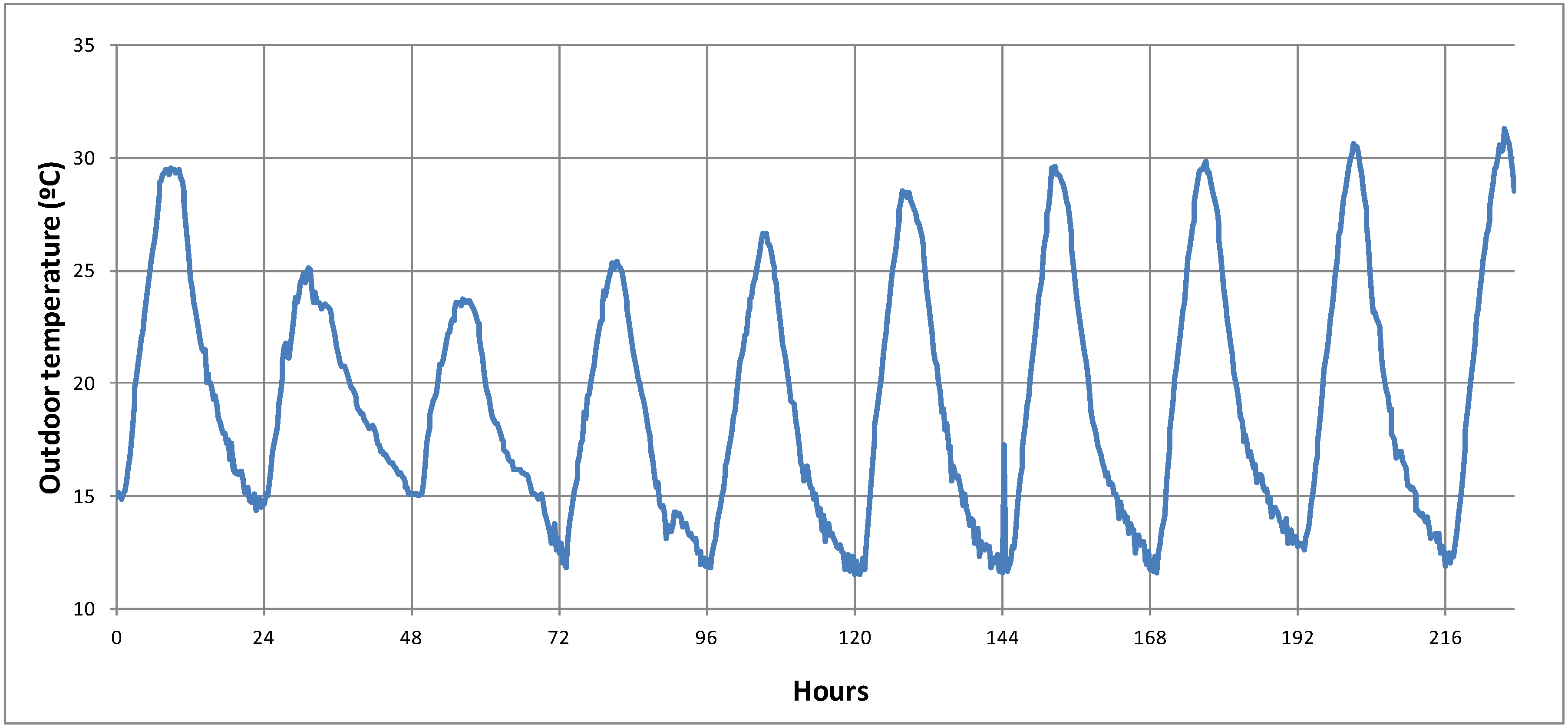
Weather conditions were simulated using data from a weather station and entering the velocities and wind directions as well as the air temperatures outside the cubicle. The boundaries of the environment were surfaces defined as velocity-inlet and pressure-outlet, through which air entered and exited, respectively. The experimental outdoor temperature data from the weather station are shown in
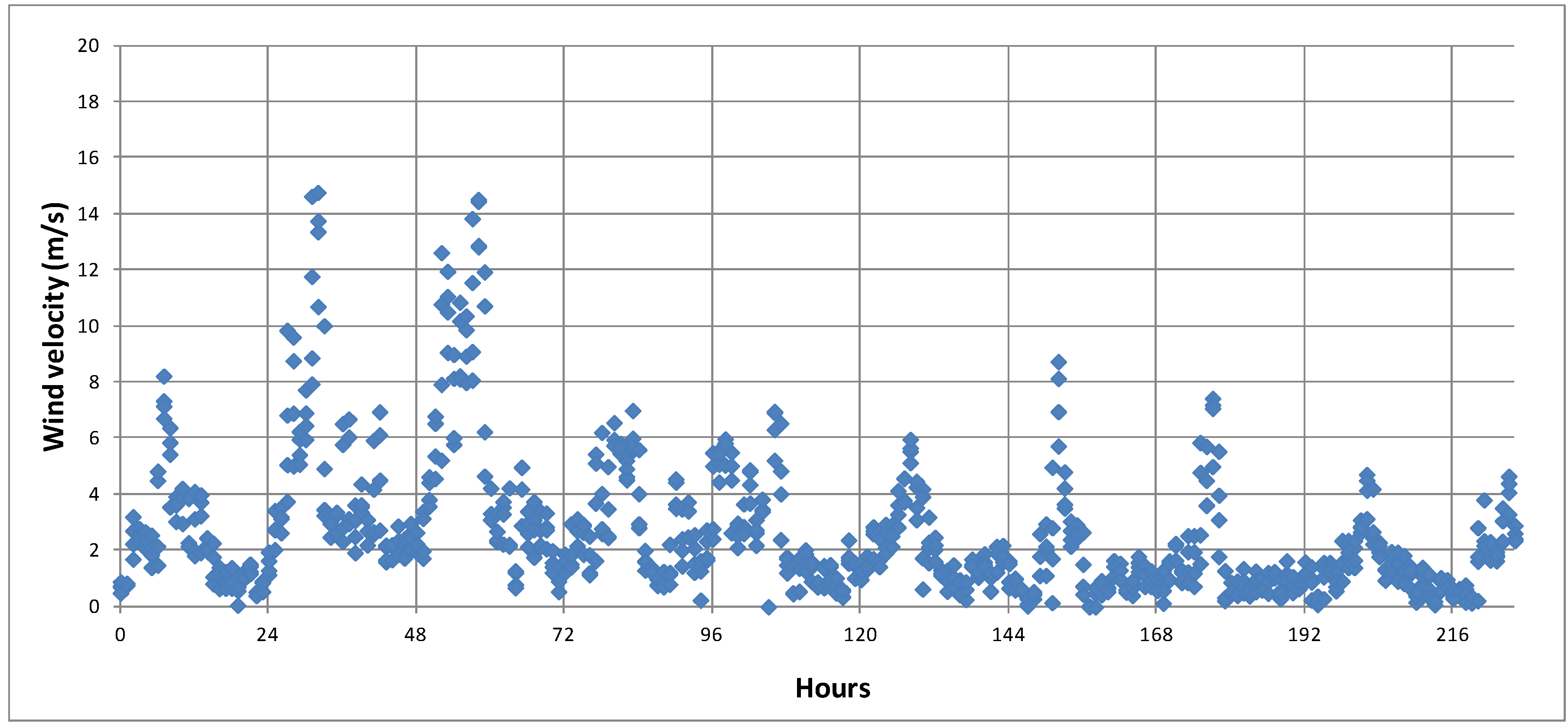
Figure 4. These data are crucial for the simulation of the environment behaviour. The wind velocity is another important parameter to take into account in the modelling of the environment. This velocity was measured and the data are shown in
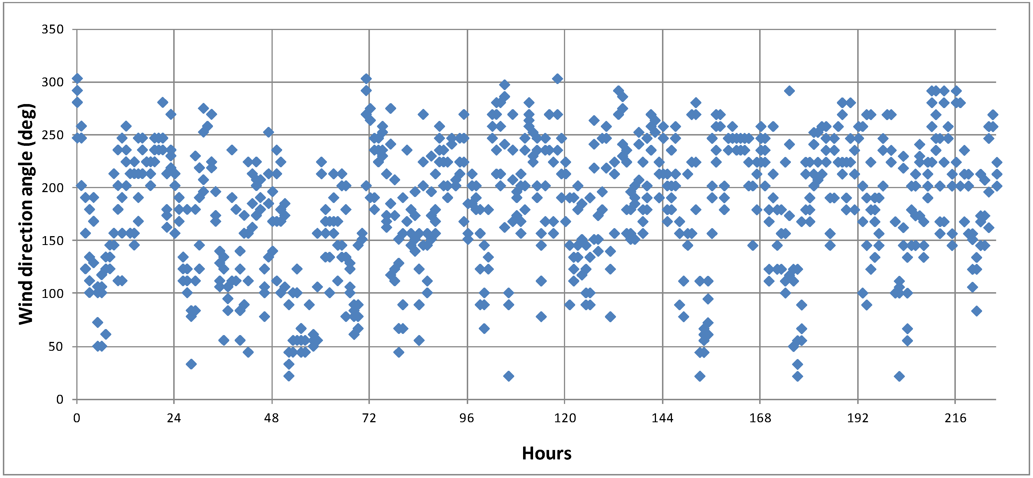
Figure 5. High and variable wind velocities can be observed around midday whereas the velocities remain stable the rest of the time. The wind direction angle was also measured in the weather station and it was introduced in the simulation as a boundary condition, considering the north direction as 0 degrees. The experimental data are shown in
Figure 6. We see that the wind angle is significantly more chaotic than most of the boundary conditions and it is difficult to draw conclusions about its behaviour. The simulated atmospheric conditions were updated every hour, thereby making them coincide with the data obtained by the air station, which were averaged from the readings of that time interval.
Figure 4.
Outdoor temperature data measured in the weather station.
Figure 4.
Outdoor temperature data measured in the weather station.
Figure 5.
Wind velocities measured in the weather station.
Figure 5.
Wind velocities measured in the weather station.
Figure 6.
Wind direction angle measured in the weather station.
Figure 6.
Wind direction angle measured in the weather station.
Solar radiation was introduced using the solar irradiation calculator of ANSYS Fluent, which imposed the incident radiation on the exposed surfaces according to the position of the sun, which varies as a function of time. The position of the sun depends on the day of the year and geographical coordinates, which were also entered into the solar irradiation calculator. The geographical coordinates where the cubicle was placed were latitude 42.13 and longitude 8.62.
4. Results and Discussion
The experimental system recorded data for several months during the year 2011. As it was difficult to take into account the variability of weather, a sunny weather period of ten days in the month of October was chosen to simulate climate conditions more accurately. Below, the proposed model is applied in a simulation of the experimental cubicle exposed to the measured weather conditions, and the results are compared with experimental data to contrast the proposed model and of the assumptions made. Subsequently, the parameters that affect the thermal behaviour of the system are presented and discussed in more depth. In addition, various figures are shown to analyse the variations of temperature fields and the PCM evolution throughout a typical day. Then, a similar simulation is performed in a cubicle in which panels exposed to solar radiation (south, east and west) consist of a mixture of concrete and 5% PCM. The results of this simulation are shown and compared with the results of the simulation without PCM.
4.1. Comparison of Experimental and Simulation Results
Several measurements were taken in the experimental cubicle; the most representative measurements are the temperatures of the internal and external surfaces of the panels. As commented in
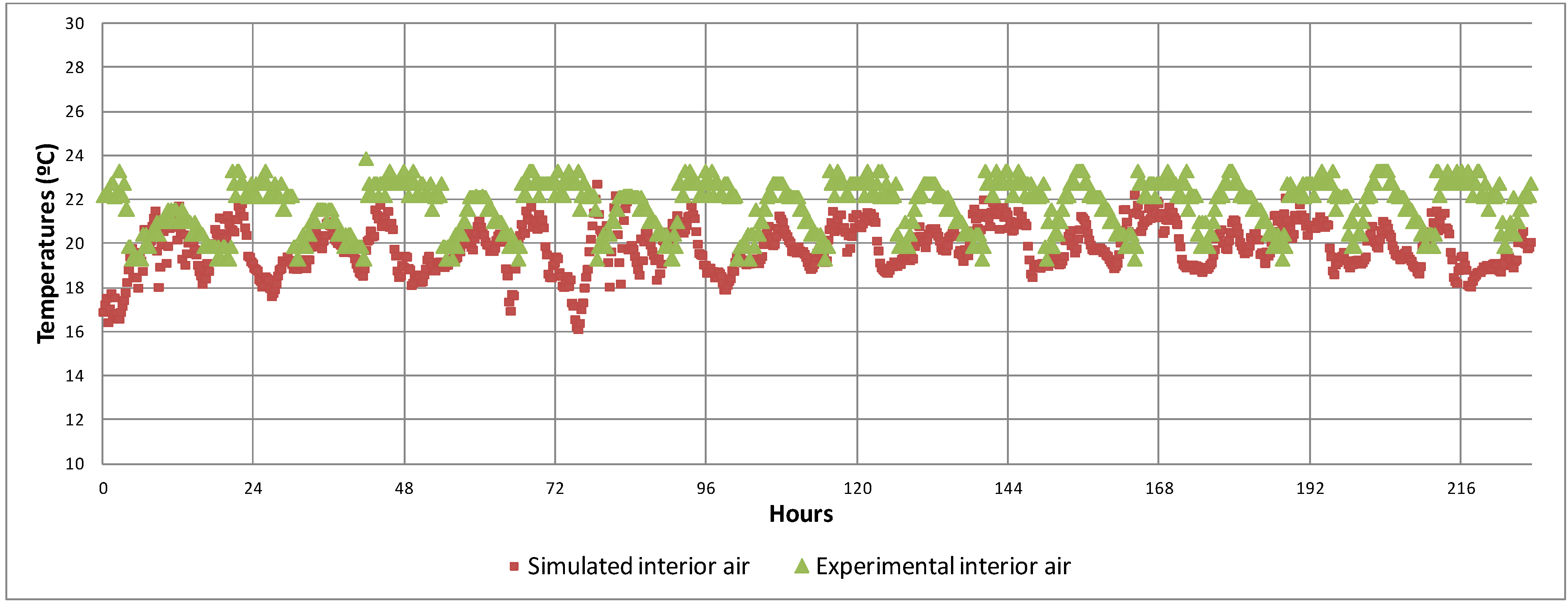
Section 2, the heat pump is programmed to maintain a temperature of 20 °C inside the cubicle by working with on-off regulation. The temperature of the air inside the cubicle, which is measured by a set of thermometers, is shown in
Figure 7 and compared with the predicted values (calculated as the average temperature inside the cubicle).
Figure 7.
Measured and predicted temperatures of the air inside the cubicle.
Figure 7.
Measured and predicted temperatures of the air inside the cubicle.
Measurements and predictions show a reasonably similar pattern, however the predicted temperatures are generally 1–2 degrees lower. This could be because the actual efficiency of the heat pump is lower than the specifications. In some instants of the simulation the temperature drops to 16 degrees, this is caused by the time step size which causes excessive cooling time.
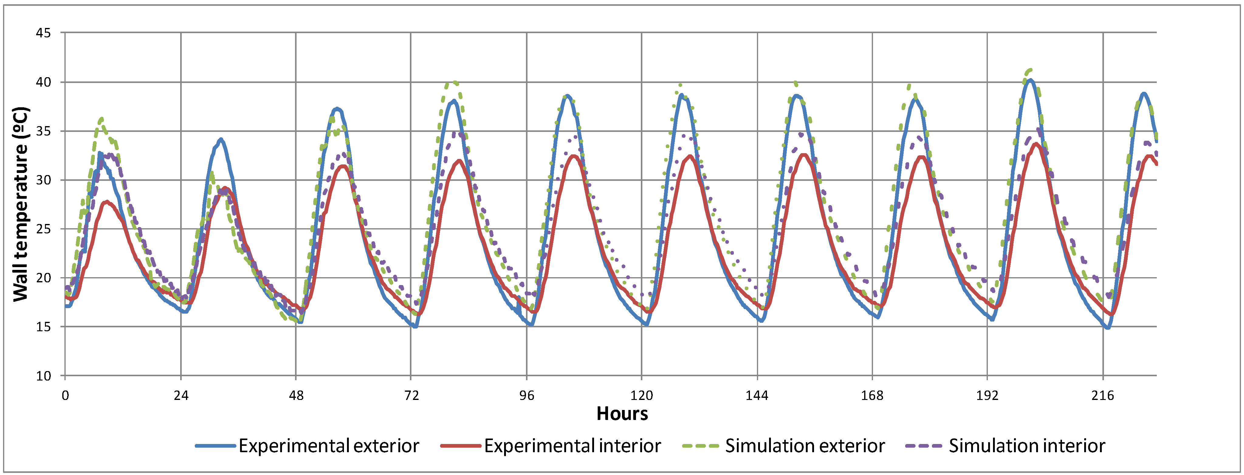
As the south wall receives the most solar radiation, the validation of the CFD simulation was performed by comparing the temperatures of this wall.
Figure 8 shows the experimental south wall temperatures during ten consecutive days and the same temperatures predicted by the simulation for the same period, which begins at 8:00 AM on October 5th.
Figure 8.
Measure and predicted temperatures of the south wall of the cubicle.
Figure 8.
Measure and predicted temperatures of the south wall of the cubicle.
The overall behaviour of the two temperatures (internal and external) follows a reasonably similar pattern throughout the simulation period. The heating and cooling of the outer surface occur rapidly during daylight hours; however, the cooling is slower at night. The temperature of the inner surface responds to external changes following the pattern of the outer surface variations with a certain delay and slower temperature changes. As the simulation begins with initial values different from the real values, the predicted temperatures do not closely match the measured temperatures during the two first simulated days. In addition, the simulation predicts slightly higher maximum temperatures than are seen in the experimental data. This effect may be due to the assumed value of the concrete reflectivity, which may produce an excess of absorption of radiation. We should mention that in the experimental cubicle, the thermocouples are located at a depth a few millimeters from the surface, while the simulation shows the surface temperatures.
Figure 9.
Measured vs. predicted thermal consumptions per hour in the heat pump.
Figure 9.
Measured vs. predicted thermal consumptions per hour in the heat pump.
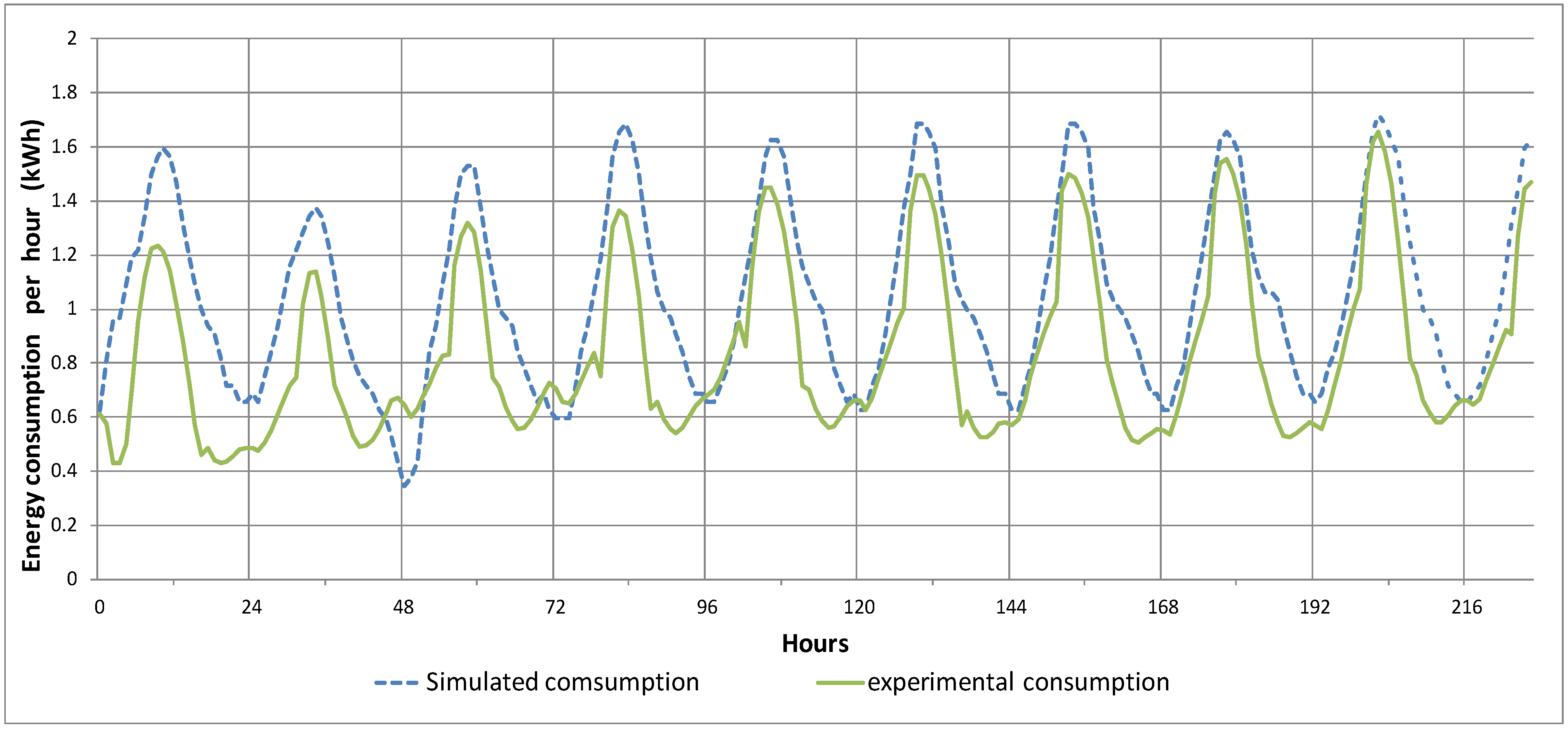
The energy consumption of the heat pumps is a useful parameter to quantify the energy saving.
Figure 9 compares the predicted values of thermal energy consumed per hour with the data registered by the consumption meter. The first conclusion we can draw from this comparison is the higher consumption predicted by the simulation than the experimental one in most days. This is consistent with the temperatures inside the cubicle shown in
Figure 7 which may be caused by a lower efficiency of the real cooling system.
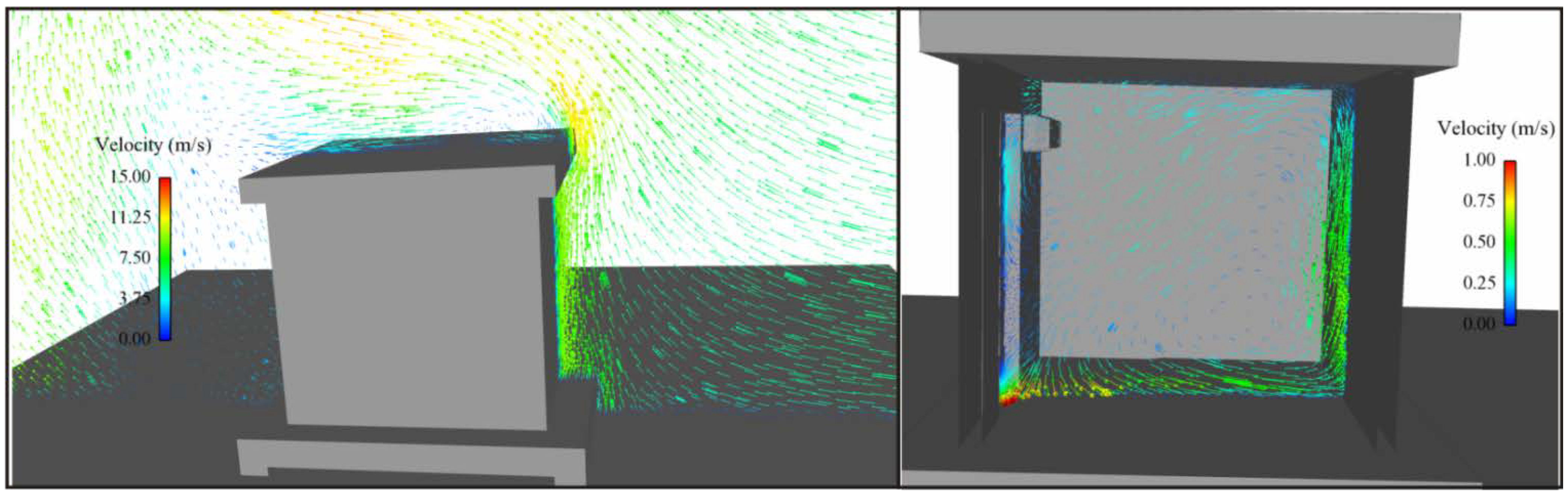
Figure 10 shows the movement of air outside the cubicle due to the wind and inside the cubicle due to the air stream created by the heat pump. These air movements play an important role in enhancing the heat convection that cools the walls.
Figure 10.
Vector fields of external and internal air velocities (m/s).
Figure 10.
Vector fields of external and internal air velocities (m/s).
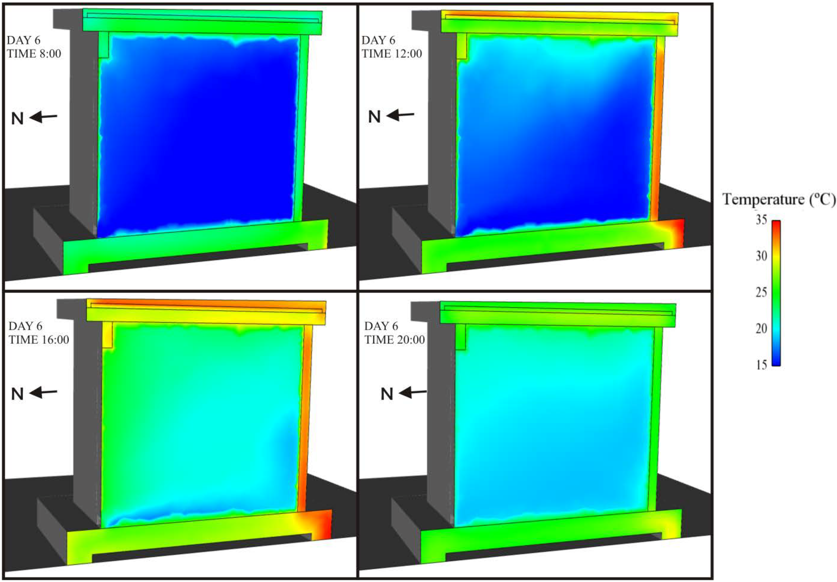
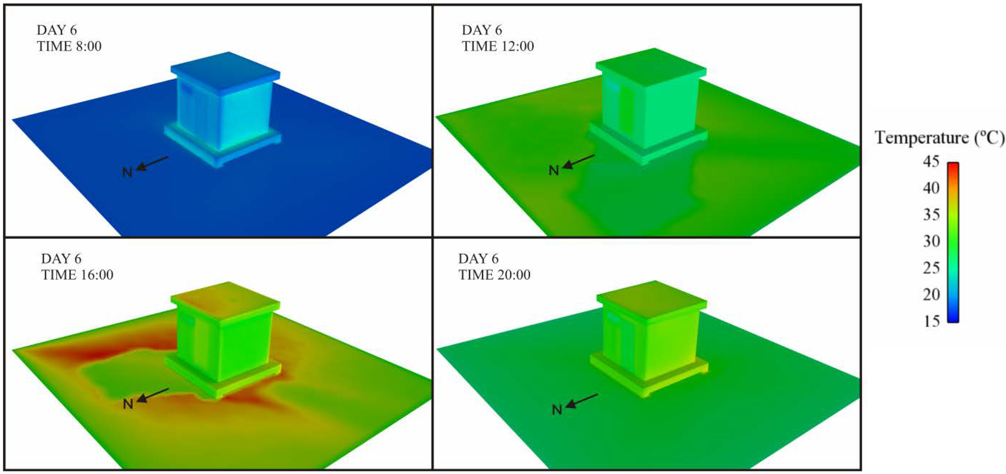
The surfaces exposed to direct sunlight experience significant heating as a result of the solar radiation.
This heat is transferred by conduction through the walls and by convection to the air near the wall surfaces.
Figure 11 shows the variation of the temperature in the walls and floor of the cubicle due to the variation in sun position during the day and
Figure 12 shows the variation between the air temperature and the wall temperature inside the cubicle.
Figure 11.
Evolution of the temperature field of the cubicle surfaces.
Figure 11.
Evolution of the temperature field of the cubicle surfaces.
Figure 12.
Evolution of the temperature field inside the cubicle and inside the walls.
Figure 12.
Evolution of the temperature field inside the cubicle and inside the walls.
4.2. PCM Simulation
The same days shown in
Figure 8 were simulated with the south, east and west panels (those exposed to solar radiation) consisting of a mixture of concrete and 5% PCM. In this way, the effect of the PCM on the thermal behaviour was evaluated; the results are analysed below.
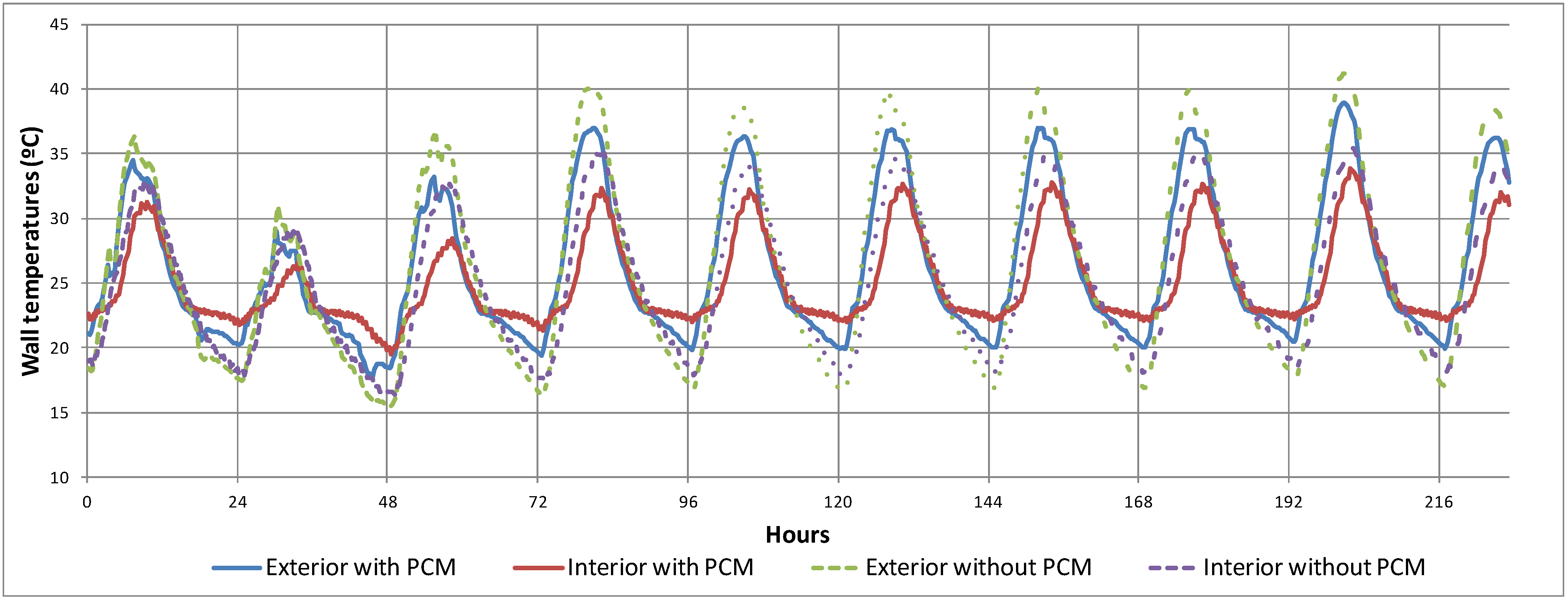
In
Figure 13, the daily cycles of the internal and external surface temperatures of the south wall are shown. Although some irregularities are observed during the simulated period, some general conclusions regarding the different thermal behaviour of the materials can be drawn. The most notable finding is that the maximum and minimum temperatures (internal and external) are clearly damped on the PCM concrete wall. The maximum and minimum values are reduced and increased, respectively, by approximately three degrees Celsius in the walls with PCM. Another clear difference observed in the inner surface temperature histories is that during cooling, the PCM acts when the phase change temperature is reached, reducing the slope of the interior temperature variation (cooling rate). This is because the PCM solidifies, and this process releases the energy stored as latent heat as the temperature remains constant. Therefore, the PCM slows the cooling rate of the wall. In the heating process, the PCM slows the heating rate of the wall, but this effect is less visible in the graph because the energy input due to solar radiation is relatively high.
Figure 13.
Predicted temperatures of the south wall of the cubicle in the simulation with and without PCM.
Figure 13.
Predicted temperatures of the south wall of the cubicle in the simulation with and without PCM.
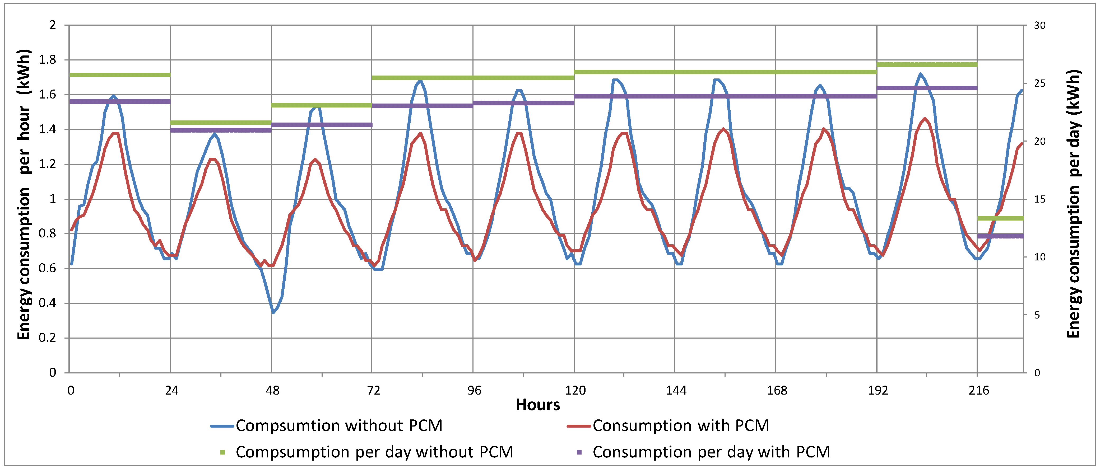
The comparison between the thermal consumption of the two simulations is shown in
Figure 14 where the evolution of the consumptions per hour and the total consumption per day are observed.
Figure 14.
Predicted thermal consumption of the heat pump of the cubicle in the simulation with and without PCM.
Figure 14.
Predicted thermal consumption of the heat pump of the cubicle in the simulation with and without PCM.
The main conclusion is the lower energy consumed in the simulation with PCM during daylight hours, which shows that the PCM stores part of the energy received by the cubicle. The difference observed during the night when the PCM releases the energy stored, thereby producing a greater consumption of the heat pump, is less significant. The amount of the overall energy saved in the case of PCM was approximately 8%. This can be clearly seen through its daily consumption.
Figure 15 represents the evolution of the air temperature and the wall temperatures inside the cubicle with PCM. The temperature changes inside the walls are milder than in the cubicle without PCM (
Figure 12).
Figure 15.
Evolution of the temperature field inside the cubicle and inside the walls in the PCM simulation.
Figure 15.
Evolution of the temperature field inside the cubicle and inside the walls in the PCM simulation.
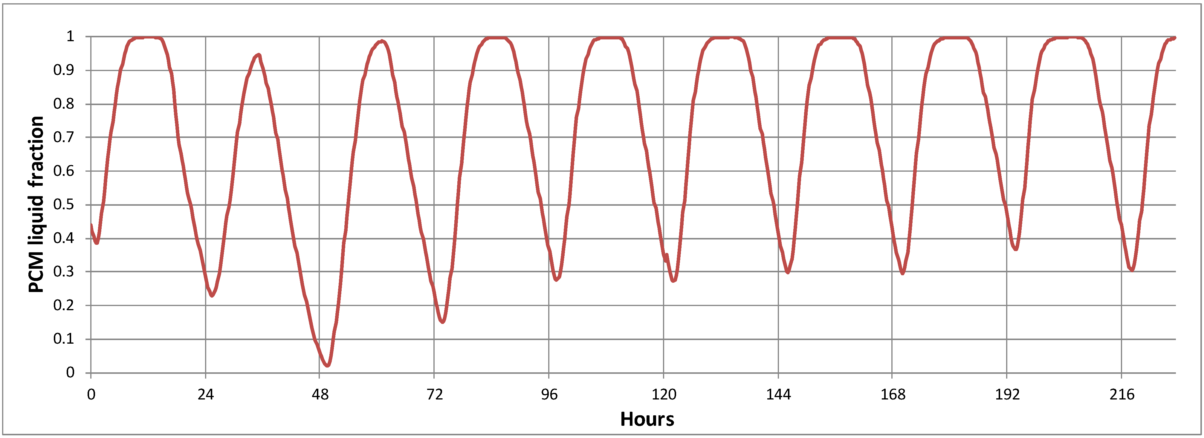
Figure 16 shows the PCM liquid fraction [
in Equations (1) and (2)], which increases when the wall receives heat and its temperature reaches the phase change temperature while absorbing the energy required to melt the PCM. This process stops when the PCM totally liquefies (
= 1). During the cooling process, the heat that has been absorbed by the PCM is released while the liquid fraction decreases (PCM solidification).
Figure 16.
Evolution of the PCM liquid fraction.
Figure 16.
Evolution of the PCM liquid fraction.
Most of the days the PCM is totally charged (
= 1) during the day; however, it does not fully discharge overnight (
> 0). This means the amount of PCM is enough to hold a more severe nocturnal cooling. The environmental temperatures in the second and third day are moderate during daylight hours (
Figure 4), so the PCM liquid fraction is less than one, due to the lower heating of the walls.
The wall temperatures reach values clearly higher than the phase change temperature during the day and lower during the night. This indicates the phase change temperature is appropriate to this climate, however, as the PCM does not completely solidify during the night, a PCM with a lower phase change temperature may work better and it may be fully discharged (solidified), which results in a greater heat storage capacity and lower temperature variations inside the cubicle.
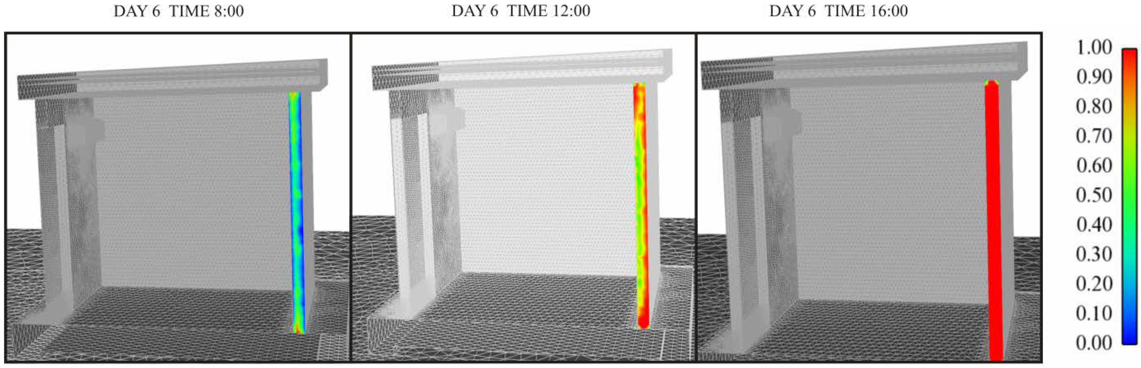
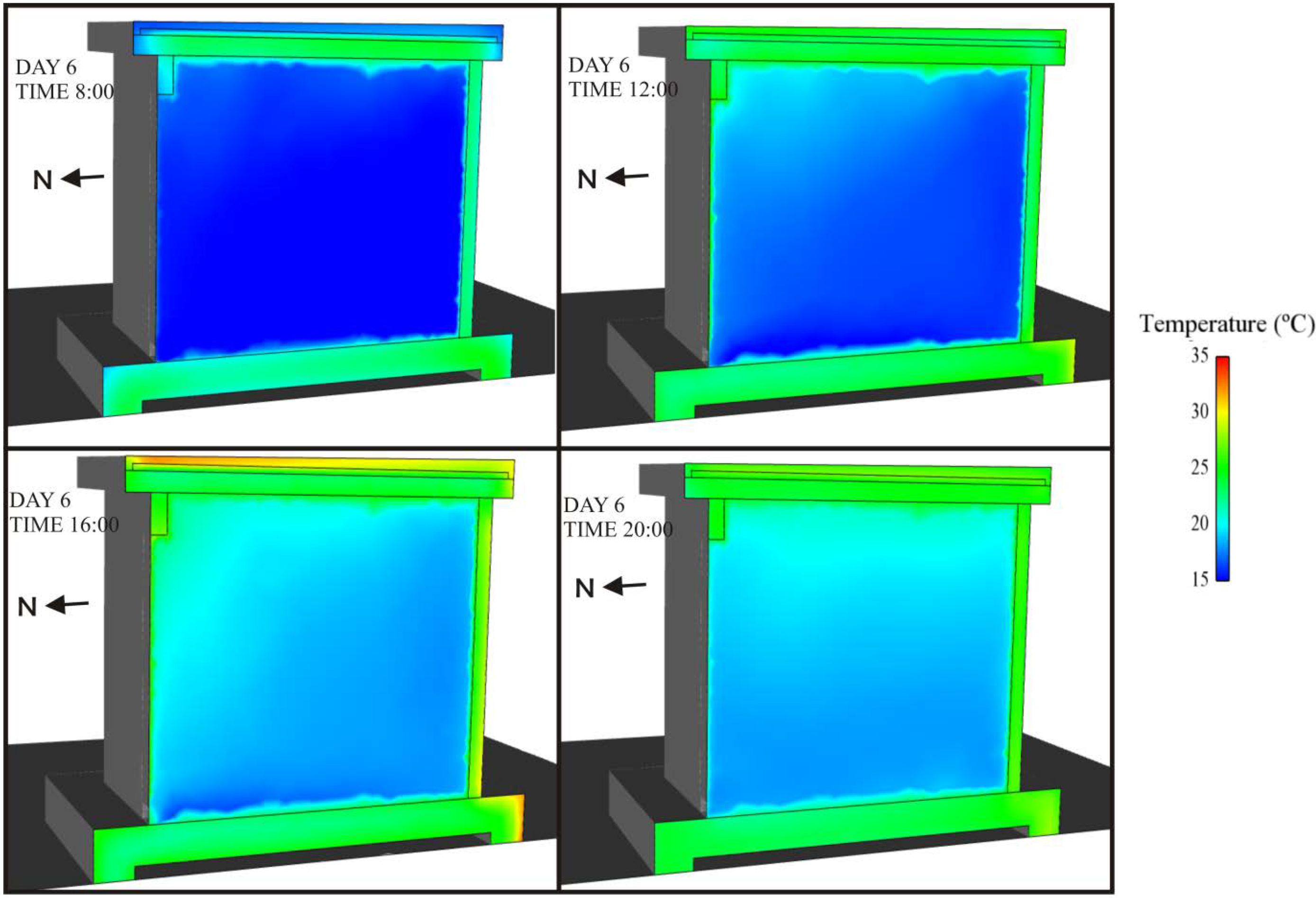
Figure 17 shows the variation of the liquid fraction of the PCM (
in Equations (1) and (2) in
Table 2) in the south wall, which melts as the wall receives energy from solar radiation. The image of “Time 8:00”, which represents one of the last moments before sunrise (when the night cooling ends), shows most of the wall section with a liquid fraction greater than zero (as shown in
Figure 16). However, at “Time 16:00” (when the sun is still heating the wall), the PCM liquid fraction is equal to one in the whole wall section. This means the PCM effect disappears before the heating process ends.
Figure 17.
Evolution of the PCM liquid fraction in the south wall.
Figure 17.
Evolution of the PCM liquid fraction in the south wall.
5. Conclusions
In this paper, we have presented a CFD model to simulate experimental buildings in order to study their behaviour under changing climatic conditions depending on their construction materials. The simulation allows an in-depth analysis of the main parameters that affect the behaviour of the building and helps predict the results of different experiments. The proposed model’s simulation results have been compared with experimental data, and the results have been found to be reasonably similar.
The measured variations in the meteorological conditions of wind and sun over several consecutive days have been reproduced; the heat pump inside the cubicle and the thermal storage capacity of the walls have been simulated with the use of CFD simulation techniques and programming of user defined functions (UDF). The main difficulty in the modelling effort is to reproduce the climatic variation at every instant; there are limitations to correctly simulating the climatic conditions and intermittent rain clouds, which can lead to the implementation of approximate solutions. As a result, in this study only clear days have been simulated. Another limitation is the starting point of the simulation, as the initial values of the variables do not match the experimental values; the first day of the simulation is a transition period to allow for appropriate values on subsequent days.
The comparison of the simulation results of the cubicles with PCM and without PCM shows that the PCM provides temperature stability and resistance to the changes in external conditions, which makes these materials suitable for increasing the thermal comfort of buildings.


