On Space-Time Resolution of Inflow Representations for Wind Turbine Loads Analysis

Abstract

Efficient spatial and temporal resolution of simulated inflow wind fields is important in order to represent wind turbine dynamics and derive load statistics for design. Using Fourier-based stochastic simulation of inflow turbulence, we first investigate loads for a utility-scale turbine in the neutral atmospheric boundary layer. Load statistics, spectra, and wavelet analysis representations for different space and time resolutions are compared. Next, large-eddy simulation (LES) is employed with space-time resolutions, justified on the basis of the earlier stochastic simulations, to again derive turbine loads. Extreme and fatigue loads from the two approaches used in inflow field generation are compared. On the basis of simulation studies carried out for three different wind speeds in the turbine’s operating range, it is shown that inflow turbulence described using 10-meter spatial resolution and 1 Hz temporal resolution is adequate for assessing turbine loads. Such studies on the investigation of adequate filtering or resolution of inflow wind fields help to establish efficient strategies for LES and other physical or stochastic simulation needed in turbine loads studies.

1. Introduction

No systematic studies have been conducted to date that have addressed the issue of efficiency of spatio-temporal resolution in generating inflow velocity fields for purposes of estimating accurate load statistics for today’s large utility-scale wind turbines. The present study addresses this issue by making use of conventional stochastic simulation of stationary Gaussian fields using Fourier methods for neutral atmospheric stability conditions. These simulated wind fields have characteristics that are similar to what is required per turbine design guidelines [1].

Historically, inflow wind generation for wind turbine loads studies has relied most commonly on stochastic simulation using spectral approaches [2] that yield Gaussian velocity fields. Lately, however, other procedures such as a continuous-time random walk (CTRW) model [3] are being proposed to describe a broader class of stochastic processes, and large-eddy simulation (LES) is being employed (as in the current study) to represent inflow turbulence. In the present study, we employ stochastic simulation for the required inflow wind field generation and study loads on a utility-scale wind turbine (rated at 5 MW) that has a hub height of 90 m and a rotor diameter of 126 m. In the design of wind turbines, modeling of turbulence is of great importance and alternative procedures are employed to simulate inflow wind velocity fields and evaluate wind turbine ultimate and fatigue limit states. Our interest in this study is in determining an acceptable frequency resolution for inflow turbulence generation so that resulting turbine load statistics (related to extremes or ultimate limit states as well as fatigue) can be predicted with little loss of accuracy compared to more finely resolved flow fields. Spectral filtering of the “base inflow” generated at 32 Hz sampling is applied in the frequency domain to generate samples with some intentional loss of high-frequency energy. Likewise, spatial grid resolution on the rotor plane (represented by a square, 140 m on side) is varied to different degrees of coarseness and loads studied following aeroelastic simulation. The dynamic characteristics of turbine loads including the flapwise bending moment at a blade root and the fore-aft tower base bending moment are studied.

From the study of turbine load statistics based on stochastic simulation of inflow, we establish the degree of resolution in space and time that is necessary for reasonably accurate extreme and fatigue load predictions in design. This same level of spatial and temporal resolution is next employed in studies involving the use of large-eddy simulation (LES) for load computations. Load statistics from stochastic simulation and LES are then compared.

2. Stochastic Simulation: Inflow and Turbine Loads

A Fourier-based stochastic turbulence simulation procedure was used to generate the “base inflow” for this study. The code, TurbSim [4], was used to stochastically generate full spatio-temporal wind velocity fields. Kaimal power spectral density (PSD) functions were used for the turbulence generation [1]. These spectra (modified from the original by Kaimal et al. [5]) can be expressed as follows:

$$\frac{f·S_k\left(f\right)}{{\sigma }_k^2}=\frac{4f·L_k/V_{hub}}{{\left(1+6f·L_k/V_{hub}\right)}^{5/3}}$$

(1)

where f represents frequency in Hz; k is an index referring to the direction of the wind velocity component (k is set equal to 1, 2, or 3 for the longitudinal, lateral, and vertical components, respectively); $S_k\left(f\right)$ is the single-sided power spectral density function for velocity component, k; ${\sigma }_k$ is the standard deviation for velocity component k; $L_k$ is the integral scale parameter for velocity component, k; and $V_{hub}$ is the ten-minute average hub-height longitudinal wind speed. In wind turbine design, values for the three wind velocity component standard deviations and integral scale parameters are specified in the IEC 61400-1 guidelines [1].

An exponential coherence function specified in the IEC 61400-1 guidelines [1] was also used in this study. This function is expressed as follows:

$$Coh(r,f)=exp\left[-12{\left({\left(f·r/V_{hub}\right)}^2+{\left(0.12r/L_c\right)}^2\right)}^{0.5}\right]$$

(2)

where $Coh(r,f)$ is defined here as the magnitude of the complex cross-spectral density function of the longitudinal wind velocity component at two spatially separated points divided by the square root of the product of the autospectra at the two points; r is the magnitude of the projection of the separation vector between the two points onto a plane normal to the longitudinal wind direction; and $L_c$ is the coherence scale parameter.

The Normal Turbulence Model (NTM) [1] with a reference turbulence intensity of 16% (corresponding to Wind Turbine Class A) was used to generate the inflow velocity field. Using the NTM, the power spectra, the coherence functions, and the reference turbulence intensity, full wind fields were stochastically generated on a rotor plane for the wind turbine selected. A time step of 0.03125 s (representing 32 Hz sampling) was used to generate the “base inflow” turbulence. Table 1 summarizes various parameters and their values used in the inflow simulation with TurbSim. These inflow fields for three different wind speeds were filtered in the frequency domain using low-pass filters with cut-off frequencies set at 16 Hz, 8 Hz, 4 Hz, 2 Hz, 1 Hz, 1/2 Hz, 1/4 Hz, and 1/8 Hz.

Table 1. Parameters and values used in inflow turbulence field simulations.

Parameters	Values
Hub height (m)	90
Rotor diameter (m)	126
Hub-height wind speed (m/s)	12, 15, 18
Base inflow sampling rate (Hz)	32
Low-pass cut-off frequency (Hz)	16, 8, 4, 2, 1, 0.5, 0.25, 0.125
Grid (y × z)	13 × 13, 11 × 11, 9 × 9
Surface roughness (m)	0.1

Table 1. Parameters and values used in inflow turbulence field simulations.

Parameters	Values
Hub height (m)	90
Rotor diameter (m)	126
Hub-height wind speed (m/s)	12, 15, 18
Base inflow sampling rate (Hz)	32
Low-pass cut-off frequency (Hz)	16, 8, 4, 2, 1, 0.5, 0.25, 0.125
Grid (y × z)	13 × 13, 11 × 11, 9 × 9
Surface roughness (m)	0.1

The rotor plane of the selected 5-MW turbine model [6] with a rotor diameter of 126 m is represented in separate analyses by 13 × 13, 11 × 11, and 9 × 9 grids that cover a two-dimensional square of side 140 m, centered at the rotor hub. The 5-MW wind turbine model is intended to represent larger utility-scale wind turbines that are likely to become more commonly used; it is commonly referred to as the NREL (National Renewable Energy Laboratory) 5-MW “baseline” wind turbine model. This model is used in all our aeroelastic response simulations. The turbine is a variable-speed, collective pitch-controlled machine. Two different turbine loads are studied; these include the flapwise bending moment at a blade root (FBM) and the tower base fore-aft bending moment (TBM). Ten-minute time series of these loads are simulated using the aeroelastic simulation tool, FAST [7], developed at NREL. The open-source software, FAST, employs a modal multi-body representation for the wind turbine system and, in this study, aerodynamic forces on the rotor are computed using the blade element momentum method and used in time-domain analysis of the turbine response.

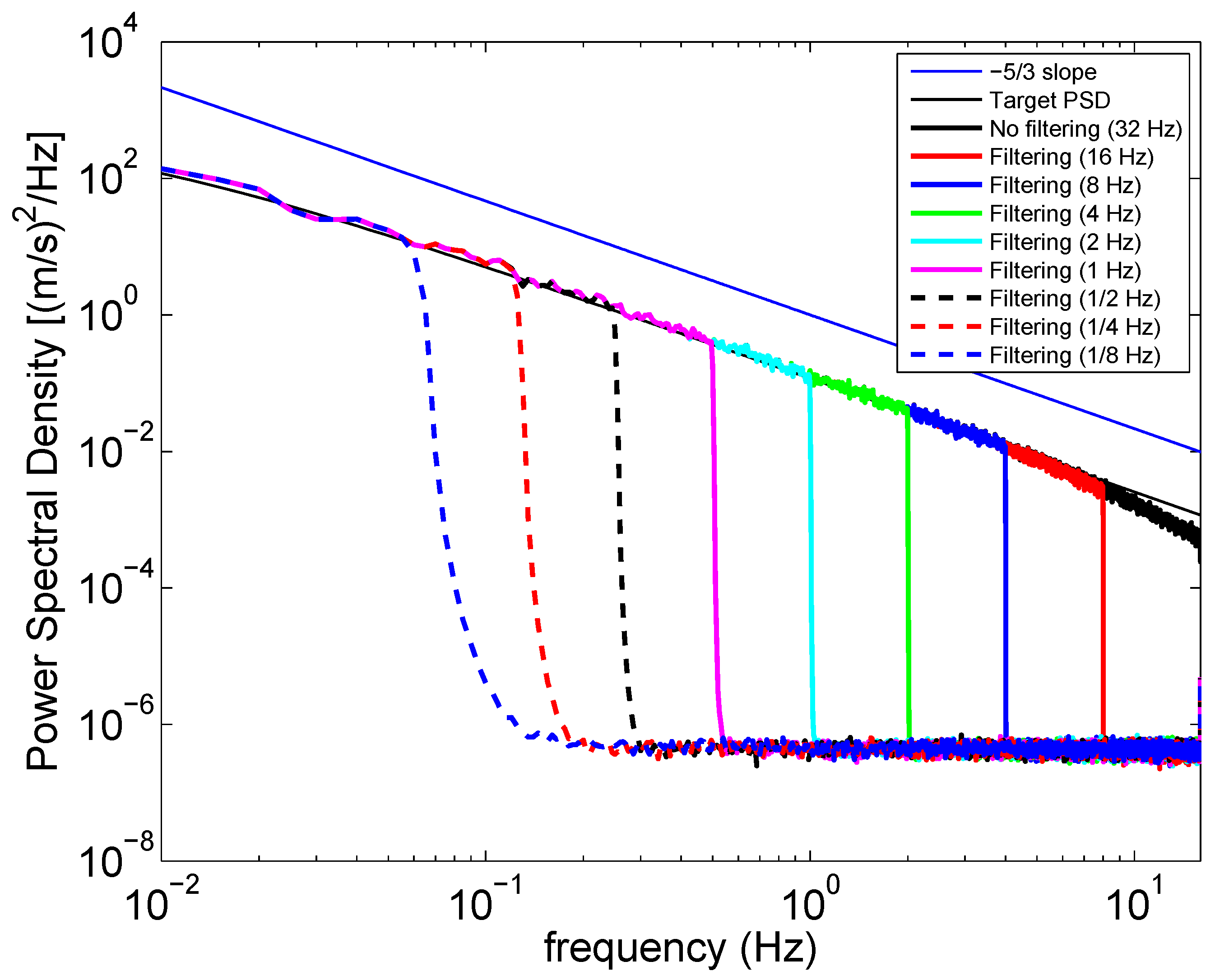
2.1. Filtering of Inflow Turbulence

To the base inflow (at a 32 Hz sampling rate) obtained from TurbSim, a low-pass filter was applied in the frequency domain with cut-off frequencies defined as given in Table 1. Power spectral density (PSD) functions computed for the various filtered longitudinal wind velocity time series at hub height are presented in Figure 1 for a ten-minute average hub-height wind speed of 12 m/s. These estimated PSDs are based on an ensemble of 15 ten-minute simulations in each case. The PSDs are shown only up to 16 Hz, the Nyquist frequency for the “base inflow” case. The log-log plot shows that all the inflow time series, with or without the filtering, follow Kolmogorov’s −5/3 power law for scaling of turbulence in the inertial subrange. The target Kaimal PSD for longitudinal turbulence at hub height is also shown in Figure 1—the simulated PSD for the unfiltered case matches the target spectrum well; it is slightly deficient in power at frequencies above around 8 Hz. As increased filtering is applied, the estimated PSDs exhibit energy deficiency at lower and lower frequencies as expected.

Figure 1. Target Kaimal PSD and estimated PSDs from unfiltered and filtered simulated hub-height longitudinal velocity time series (for a ten-minute mean wind speed of 12 m/s).

Figure 1. Target Kaimal PSD and estimated PSDs from unfiltered and filtered simulated hub-height longitudinal velocity time series (for a ten-minute mean wind speed of 12 m/s).

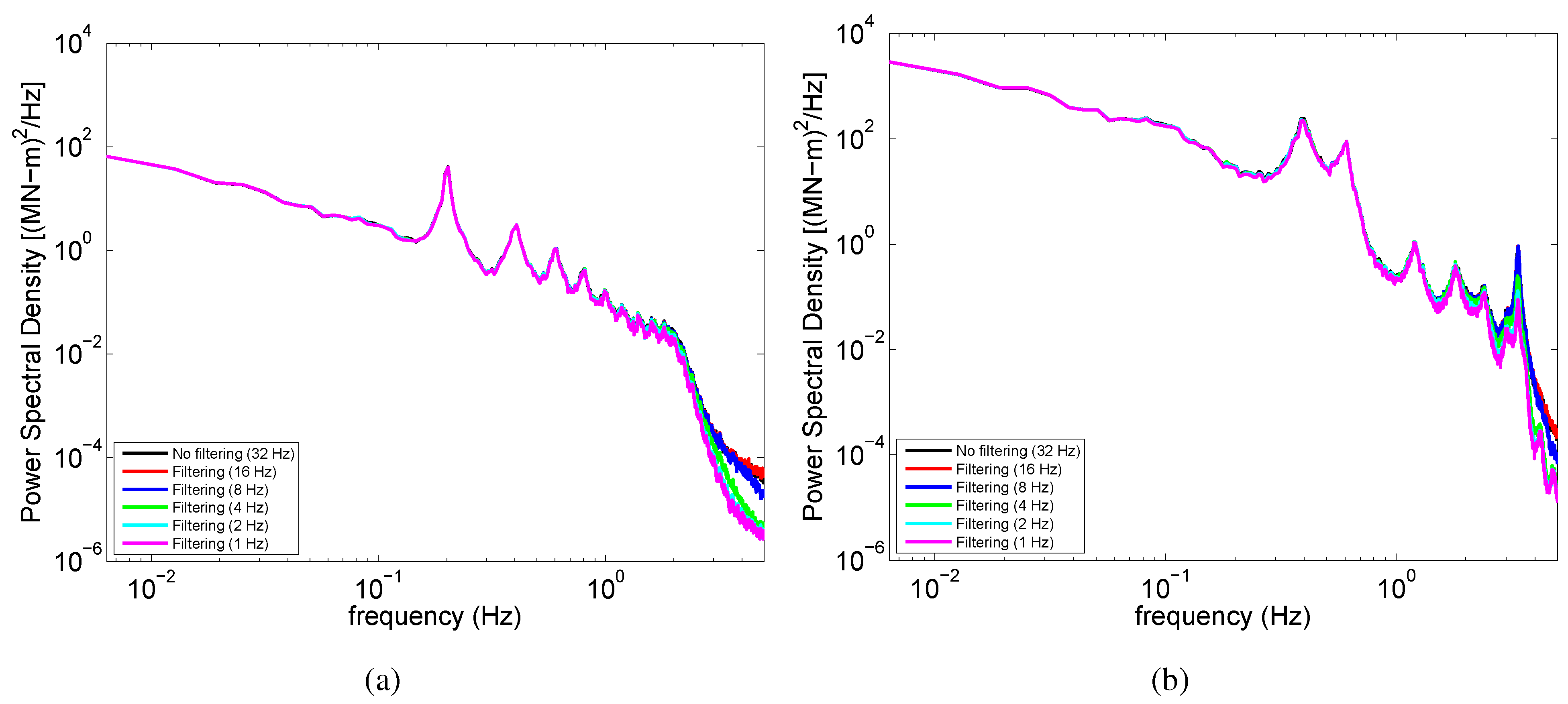
2.2. Power Spectral Density Functions for Turbine Loads

Gravitational, inertial, and aerodynamic forces all contribute to the overall loading on wind turbine components [8]. Gravitational loading refers, for example, to the force on blades that causes periodic loading once per revolution; these forces are experienced at the rotor’s rotational frequency denoted by 1P (in our case, 1P corresponds to approximately 0.2 Hz). Inertial loading is caused by accelerations or decelerations in the blade rotation. Centrifugal forces that also result have two components; one is spanwise and the other is in a normal direction. These latter forces influence the flapwise bending moment (FBM) on a blade. Finally, aerodynamic loads resulting from the inflow influence turbine loads. It is instructive to study PSDs of turbine loads in order to assess the dynamic behavior of the wind turbine in our study and to note the influence of different forces, often evident in distinct spectral peaks.

Power spectra for FBM and TBM are presented in Figure 2. The loads data for these PSDs were generated from a full-field inflow simulation on a 9 × 9 grid with hub-height ten-minute mean wind speed of 12 m/s. Because the natural modes of vibration for our wind turbine model suggest that all important blade and tower vibration modes occur at frequencies below 5 Hz, log-log plots of the load PSDs were plotted only up to 5 Hz. (We note in passing that for the FAST simulation model used here, all the modes of vibration represented for the tower and blades had natural frequencies below 5 Hz. We also note that with alternative simulation models, higher frequencies of vibration might result; however, it is our expectation that turbine loads and, hence, related fatigue and extreme loads are influenced only to a small degree by these higher frequencies.)

Figure 2. Power spectral density function for FBM (a) and TBM (b) from inflow simulated on a 9 × 9 grid and with a ten-minute mean wind speed of 12 m/s.

Figure 2. Power spectral density function for FBM (a) and TBM (b) from inflow simulated on a 9 × 9 grid and with a ten-minute mean wind speed of 12 m/s.

All the PSDs discussed here were estimated based on an ensemble of 15 realizations. Peaks in the PSDs due to the rotational frequencies of the blade (1P = 0.2 Hz, 2P, and 3P) and other important resonant frequencies are evident in the plots. These plots in Figure 2 also show the load PSDs derived based on filtered inflow (at various cut-off frequencies). The 1P spectral peaks and the various resonance peaks that match natural frequencies of the turbine blades and tower are easily identified and are all captured well even with filtering down to 1 Hz.

In the FBM PSD, the presence of 1P, 2P, 3P, etc. peaks is obvious; these peaks occur due to rotational sampling of the inflow turbulence by the moving blades. A 0.6 Hz peak is an indication of the first flapwise blade bending mode. As distinct from the blade loads, PSDs for the TBM process in Figure 2 show largest peaks near the first tower bending natural frequency, slightly below 0.4 Hz.

A study of the PSDs of the tower and blade loads (for different amounts of filtering) helps explain why tower load statistics miss the target from the “base inflow” case to a greater degree than do the blade load statistics (we shall discuss this further). The PSDs clearly show that the energy (related to variance which is the area under the PSD) of the blade loads is concentrated to a relatively greater degree at the low frequencies while tower loads display energetic peaks even above 2 Hz. The dominant PSD peaks for FBM are well captured by filtered inflow; TBM spectra show a less dominant main peak and some deficient energy at a few spectral peaks above 0.4 Hz.

2.3. Turbine Load Statistics

We are interested in turbine load statistics for the various inflow time series generated. These inflow velocity time series are generated for (i) three different hub-height mean wind speeds (12 m/s, 15 m/s, and 18 m/s); (ii) three different spatial grids/samplings on the rotor plane (13 × 13, 11 × 11, and 9 × 9); and (iii) eight different filters (low-pass filters applied at 16 Hz, 8 Hz, 4 Hz, 2 Hz, 1 Hz, 1/2 Hz, 1/4 Hz, and 1/8 Hz). We estimate the standard deviation, the ten-minute extreme, and the equivalent fatigue load (EFL) for two different turbine loads (FBM and TBM). A total of fifteen realizations were used to summarize ensemble load statistics for each load for the various inflow time series. Here, we define EFL as the constant-average load amplitude that, over a fixed number of cycles (we used 1,000 as this number), causes the same fatigue damage as the variable-amplitude ten-minute load time series does. Note that for the EFL calculations, Wöhler exponents of 10 and 3 were applied for FBM and TBM, respectively.

Ensemble standard deviation estimates of the two loads studied show very slight variation with hub-height mean wind speed. The various spatial grids including the 9 × 9 grid with a 1 Hz filter do not lead to large errors in the load standard deviations for the loads relative to the “base inflow” case and finest spatial grid. Ensemble ten-minute extreme load estimates show slightly decreasing trends with increase in wind speed from 12 m/s to 18 m/s. This is expected since the turbine is pitch-controlled and has a rated wind speed of 11.4 m/s. Loads are systematically reduced for increasing wind speeds above rated due to pitching of the blades. Ensemble EFL estimates for the loads studied show increasing trends with increase in wind speed from 12 m/s to 18 m/s. For the sake of brevity, we do not elaborate on these various trends here. Later, when we discuss comparison of loads from stochastic simulation and LES, we revisit these trends in more detail. The various spatial grids and even the 9 × 9 grid with a 1 Hz filter do not lead to large errors in ten-minute load extremes for all load types. Only small differences are seen in EFL and extreme estimates with different spatial and temporal resolution of the inflow fields. For instance, FBM EFL estimates are slightly underestimated with coarser spatial grids while TBM EFL estimates are slightly overestimated with coarser grids and spectral filtering (see Table 2); similarly both TBM and FBM extremes are slightly underestimated with coarser space-time resolution. In general, even a 9 × 9 spatial grid with a 1 Hz filter does not lead to great differences in rotor and tower extreme and fatigue load statistics.

The preceding observations suggest that it may not be necessary to employ very fine spatial sampling while generating inflow turbulence to establish wind turbine loads for design. We conclude that a 9 × 9 spatial grid for this turbine rotor may be adequate for reasonably accurate load statistics. In addition, since for the loads studied, the ten-minute extreme values are larger at 12 m/s wind speed than at higher wind speeds (as was also seen in a previous study [9]), further discussions on filtering will focus on the inflow wind velocity time series with a mean hub-height wind speed of 12 m/s.

Table 2. Turbine load ensemble statistics for a hub-height mean wind speed of 12 m/s (based on 15 realizations).

Grid, filtering	FBM (kN-m)	FBM (kN-m)	TBM (kN-m)	TBM (kN-m)
	10-min extreme	EFL	10-min extreme	EFL
13 × 13, 32 Hz	12,979	5,656	82,295	12,585
9 × 9, 1 Hz	12,789	5,369	80,901	12,719

Table 2. Turbine load ensemble statistics for a hub-height mean wind speed of 12 m/s (based on 15 realizations).

Grid, filtering	FBM (kN-m)	FBM (kN-m)	TBM (kN-m)	TBM (kN-m)
	10-min extreme	EFL	10-min extreme	EFL
13 × 13, 32 Hz	12,979	5,656	82,295	12,585
9 × 9, 1 Hz	12,789	5,369	80,901	12,719

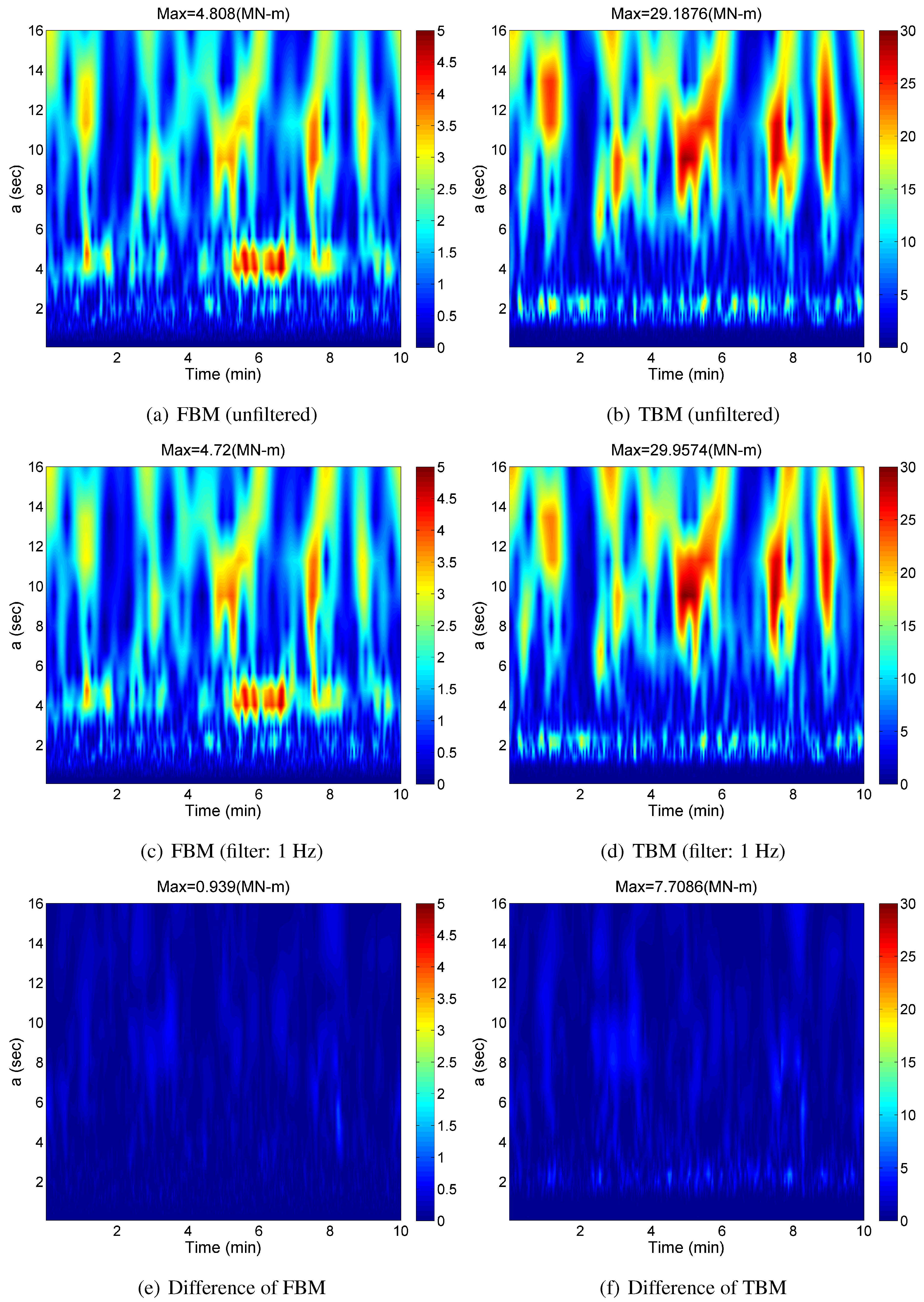
2.4. Wavelet Analyses of Turbine Loads

As has been discussed by Kelley [10], time-frequency analysis using continuous wavelet transforms can help study energetic peaks that occur coincidentally with higher-order modes that might not be detected through spectral analysis. Wavelet analysis of the loads data was performed to determine whether cutting off high frequencies in the inflow turbulence would affect turbine load characteristics in any significant way. Also, non-stationary characteristics of loads from aeroelastic simulations such as flapwise bending loads that can change based on azimuthal position of blades may be lost by relying only on spectral analysis [10]; then, wavelet analysis can again be useful.

Figure 3(a,c,e) summarizes results of the wavelet analysis for the FBM process resulting from an unfiltered inflow (13 × 13 grid and 32 Hz sampling) and an inflow filtered at 1 Hz on a 9 × 9 grid (for a hub-height mean wind speed of 12 m/s). The colorbar shows FBM wavelet coefficient values in MN-m. The x-axis shows time, while the y-axis is an indicator of the time scale of the Morlet wavelet used in the analyses. At high frequencies, the time windows are narrow; while at low frequencies, the frequency windows are narrow. In other words, long time scale values for “a” on the y-axis indicate low frequencies, while short time scales indicates high frequencies.

The wavelet plots demonstrate that there is very little difference in the blade loads that result from filtering down to 1 Hz and using a 9 × 9 spatial grid for the turbine rotor. The maximum difference in the FBM wavelet coefficients for the unfiltered and filtered cases is 0.939 MN-m for the FBM process; additionally, energetic peaks in time and at different scales are recovered quite well for the filtered flows.

Figure 3(b,d,f) summarizes results of the wavelet analysis for the tower base fore-aft moment (TBM) process for the same filtered versus unfiltered cases as were studied for FBM. The wavelet plots again show that TBM energy derived from unfiltered and filtered inflow are not very different at low frequencies; at higher frequencies (around $a=2$ s) some of load peaks are missing for the filtered inflow case.

Figure 3. Wavelet analysis of turbine blade and tower loads (for a hub-height mean speed of 12 m/s).

Figure 3. Wavelet analysis of turbine blade and tower loads (for a hub-height mean speed of 12 m/s).

2.5. Summary on Spatio-Temporal Filtering of Inflow in Stochastic Simulation

Inflow turbulence was generated based on conventional Fourier-based stochastic simulations. The base inflow was filtered with various spectral cut-off frequencies to generate inflow with different spectral content, intentionally deficient in high-frequency energy. The reason for filtering the inflow was to evaluate whether high frequencies are necessary to derive load statistics from aeroelastic simulations. The filtered and unfiltered inflow fields were applied as input to a 5-MW wind turbine model. Turbine blade and tower load time series were studied. It was found that although power spectral density functions of the filtered inflow drop considerably with greater amounts of filtering, the associated load characteristics do not change significantly with increased filtering. In general, for all of the loads studied, it was found that 9 × 9 spatial grids on the rotor plane and 1 Hz sampling could be used to estimate extreme and fatigue load statistics with reasonable accuracy. Power spectra (in Figure 2) and wavelet analyses (in Figure 3) confirmed that there were negligible losses from such filtering and revealed consistent energy distribution of loads over different frequencies.

3. Inflow Generation using Large-Eddy Simulation

Based on the preceding discussion, we arrived at adequate temporal and spatial sampling values that may be used for stochastic simulation of inflow wind velocity fields for wind turbine loads analysis. We assume that similar spatio-temporal resolution may be employed in large-eddy simulation (LES) of inflow fields and that turbine loads based on LES and stochastic simulation may then be directly compared. While LES preserves realistic atmospheric boundary layer characteristics by directly solving the nonlinear Navier–Stokes equation and the conservation of mass equation, due to the computational effort required in such simulations, less computationally intensive stochastic simulations based on Fourier techniques are commonly used in the design of wind turbines. In contrast, however, stochastic simulations have limitations especially in modeling the stratified stable boundary layer (SBL) which is often accompanied by high wind shear and low-level jets and potentially large turbine loads. The present study is being undertaken solely to evaluate wind turbine load statistics for ideal neutral conditions that can be simulated using stochastic techniques and compared with those based on LES-generated inflow. The theoretical background on the use of LES is summarized here. We briefly demonstrate, too, how inflow turbulence is generated using LES followed by fractal interpolation which is introduced to enhance the deficient high-frequency energy.

3.1. Background on Large-Eddy Simulation

Large-eddy simulation is the most efficient computational technique currently available for high Reynolds number turbulent flow simulations [11,12,13]. In this approach, one solves the filtered Navier–Stokes equation:

$$\frac{\partial \widetilde{u_i}}{\partial t}+\frac{\partial \left(\widetilde{u_i}\widetilde{u_j}\right)}{\partial x_j}=-\frac{1}{\rho }\frac{\partial \tilde{p}}{\partial x_i}+\nu \frac{{\partial }^2\widetilde{u_i}}{\partial x_j\partial x_j}+\widetilde{F_i}-\frac{\partial {\tau }_{ij}}{\partial x_j}$$

(3)

where t is time, $x_j$ is the spatial coordinate in the j direction, $u_j$ is the velocity component in that direction, p is dynamic pressure, ρ is density, ν is kinematic viscosity, and $F_i$ is a forcing term (e.g., geostrophic wind). Due to the low viscosity of atmospheric boundary layer (ABL) flows, ν is usually neglected. The tilde denotes a spatial filtering operation using a filter of characteristic width ${\Delta }_f$. For ABL simulations, ${\Delta }_f$ is typically in the order of a few meters. The effects of the subgrid scales (SGS; smaller than ${\Delta }_f$) on the evolution of $\widetilde{u_i}$ are modeled via the SGS stress term ${\tau }_{ij}$. Eddy-viscosity models (e.g., the Smagorinsky model) and their variants are the most widely used LES-SGS models for ABL simulations. For non-neutral ABL simulations, in addition to Equation (3), one also solves a filtered equation for potential temperature. Buoyancy and rotational influences are included in Equation (3).

Following the pioneering works of Deardorff in the 1970s, the field of LES of ABL turbulence (henceforth, LES-ABL) has evolved dramatically. Researchers have simulated diverse types of ABL flows (including, buoyancy-driven, shear dominated, stably stratified, transitional, and cloud-topped boundary layers; please refer to Basu et al. [14] for an abridged list of related references). Various model intercomparison studies (e.g., [15,16,17]) have identified strengths and weaknesses of different LES-SGS models, and in turn, have helped the community to develop more robust ones. Over the years, the LES-ABL approach has also found its niche in the wind energy arena. So far, it has been primarily used for turbine micrositing and wake modeling-related research (e.g., [18,19,20,21,22]). Very few published studies have reported on the application of the LES-ABL approach for wind turbine inflow generation and associated estimation of loads; the present study seeks to contribute new understanding towards this end.

3.2. Large-Eddy Simulation Code

In this study, an in-house large-eddy simulation code (called MATLES) is utilized for turbulent inflow generations. The salient features of the MATLES code are as follows: (i) the code solves the filtered incompressible Navier–Stokes equations written in rotational form; (ii) derivatives in the horizontal directions are computed using the Fourier Collocation method, while vertical derivatives are approximated with second-order central differences; (iii) de-aliasing of the non-linear terms in Fourier space is done using the 3/2 rule; (iv) an explicit second-order Adams–Bashforth time advancement scheme is used; (v) spectral cutoff filtering is used in the horizontal directions (no explicit filtering is performed in the vertical direction); (vi) only Coriolis terms involving horizontal wind are considered; and (vii) a staggered vertical grid is used. A tuning-free (dynamic) SGS model, called the locally-averaged scale-dependent dynamic (LASDD) model was used for all the simulations in the present study.

The potential of the LASDD SGS model was established in simulations of stably stratified boundary layers [23,24], neutrally buoyant boundary layers [25], an observed diurnal cycle [14], and radioactive scalar dispersion [26]. Overall, agreements between the LES-generated turbulence statistics and some well-established empirical formulations (e.g., the local scaling hypothesis) as well as theoretical predictions (e.g., Kolmogorov spectra) were remarkable. Most importantly, the LASDD SGS model performed quite well in the surface layer (in terms of proper near-wall SGS dissipation behavior). We should mention too that the MATLES code was recently utilized to set up the control case for the GEWEX Atmospheric Boundary Layer Study (GABLS) 3rd LES Intercomparison project [27].

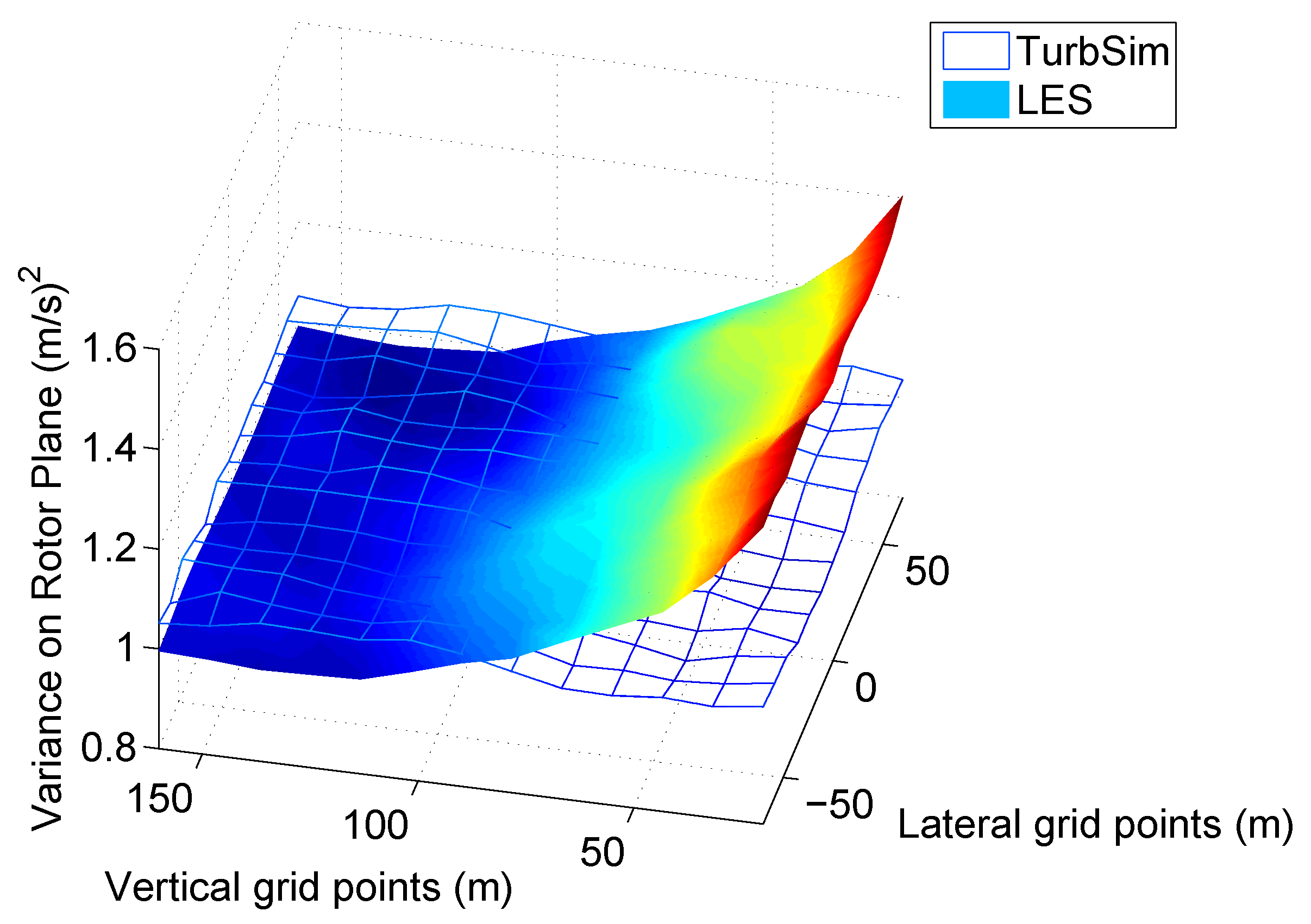
3.3. LES and Stochastic Simulation of Inflow Turbulence

In atmospheric large-eddy simulations, idealized or observed soundings (i.e., 1-D vertical profiles) of wind speed and other environmental variables (such as temperature, moisture, etc.) in conjunction with small-scale 3-D perturbations (random noise) are typically used to generate initialization fields. With the help of the Navier–Stokes equations (Equation (3)), these fields are then evolved in time under the constraints of certain large-scale forcing terms (e.g., geostrophic wind) and boundary conditions (e.g., prescribed land-surface temperature is often used as the lower boundary condition). The lower boundary condition is based on the Monin–Obukhov similarity theory with a surface roughness length of 0.1 m. Usually, it takes about an hour of simulation (depending on the characteristics of the boundary layer to be simulated) to generate realistic turbulence (i.e., for reasonable representation of the inertial range of spectra). However, it can take a few physical hours of simulation to generate quasi-steady state boundary layer conditions. For realistic neutral boundary layer simulations, one needs to run an LES code for O(12) physical hours to reach quasi-steady state conditions.

High-resolution LES runs are computationally very expensive, especially for durations of O(12) physical hours. For this reason, in the present research study, we carry out the simulations in two phases. Table 3 summarizes important computational details related to the LES runs. In Phase I, coarse runs (with a grid resolution of 20 m) of 12-hour duration are performed using a time step of 0.2 s. Then, in Phase II, the final 3-D fields from the Phase I simulations are used as initial fields and new simulations are run for 30 min (with a time step of 0.1 s). In order to create higher resolution (finer than 20 m) LES data, we first apply a cubic spline interpolation to the final 3-D fields of the Phase I simulations to produce 13.3 m resolution initial fields. Full-field wind files for 3-D velocity components are output from the last 15 min of these 30-min Phase II simulations at a frequency of 2.5 Hz (i.e., every 0.4 s). For both phases of our simulations, we used a fixed domain size of 800 m × 800 m × 1260 m.

Table 3. Specification of the LES runs.

Parameters	Phase I Simulation	Phase II Simulation
Domain size	800 m × 800 m × 1260 m	800 m × 800 m × 1260 m
Grid points	40 × 40 × 64	60 × 60 × 96
Spatial resolution	20 m × 20 m × 20 m	13.3 m × 13.3 m × 13.3 m
Time step	0.2 s	0.1 s
Run time	720 min	30 min

Table 3. Specification of the LES runs.

Parameters	Phase I Simulation	Phase II Simulation
Domain size	800 m × 800 m × 1260 m	800 m × 800 m × 1260 m
Grid points	40 × 40 × 64	60 × 60 × 96
Spatial resolution	20 m × 20 m × 20 m	13.3 m × 13.3 m × 13.3 m
Time step	0.2 s	0.1 s
Run time	720 min	30 min

Figure 4 shows a 180 m × 180 m (y-z plane) slice of the longitudinal velocity (U, including the mean and turbulence components) at a single time instant, taken from the last 15-min time series segment of the simulated wind field (with a grid resolution of 13.3 m); also shown are the 15-min time series for U versus vertical elevation (z) for points laterally separated by 150 m. In this study, we systematically varied geostrophic winds (a large-scale forcing term related to mesoscale pressure gradient forces) to obtain different hub-height wind speeds. Specifically, we considered geostrophic winds of 18 m/s, 24 m/s, and 28 m/s in the simulations.

Figure 4. Slice of the last 15 min LES-generated Phase II longitudinal velocity wind field (units: m/s).

Figure 4. Slice of the last 15 min LES-generated Phase II longitudinal velocity wind field (units: m/s).

Three sets of LES flow fields were generated for each geostrophic wind case. The 800 m × 800 m × 1260 m domain was sliced into 5 lateral sub-domains (i.e., in the y direction) yielding a total of 15 flow fields described over the turbine rotor plane. Since the w turbulence components were generated in a staggered form vertically where they were spaced between the vertical grid points of the u and v components, these w components were interpolated to the grid points of the u and v components. The entire turbulence field was interpolated to the same grid points that were used in generating the NBL inflow with stochastic simulations.

In order to provide neutral boundary layer flows from stochastic simulations whose effects on turbine loads could be directly compared with the neutral boundary layer flows generated from LES, the Fourier-based stochastic turbulence simulation code, TurbSim, was used together with target turbulence power spectra and coherence functions (the Kaimal model). The rotor plane of the selected 5 MW turbine, with a rotor diameter of 126 m, was represented as a 13 × 13 grid that covers a square area of side 140 m, centered at the rotor hub. A time step of 0.4 s was used in the NBL flow simulations to match the time step from LES. Note that the horizontal resultant of the longitudinal and lateral wind speed components at hub height (90 m) for the LES case was matched to the hub-height mean wind speed of the TurbSim simulations. A total of 15 stochastic simulations were produced and compared with the LES results.

Figure 5 shows a 3-D plot of the variance of the inflow turbulence across the rotor plane. The target variance in TurbSim, per IEC guidelines [1], is treated as constant over the entire rotor plane although this is not physically realistic. Large-eddy simulation generates turbulence at the surface and transports it upwards in neutral flows; this is also observed in nature. As a result, variance and fluxes are higher near the surface and decrease monotonically with height. Moreover, the variance and fluxes should be zero at the top of boundary layers. Figure 5 clearly demonstrates that LES is capturing the correct behavior of boundary layer characteristics. Near the hub height (90 m) of our turbine model, the variance from the LES and TurbSim procedures match reasonably well. However, while the variance from TurbSim (per IEC [1]) is constant over the entire rotor plane, the variance from LES has higher values close to the ground (20 m) and lower values above 90 m.

Figure 5. 3-D Variance of inflow streamwise turbulence across the rotor plane.

Figure 5. 3-D Variance of inflow streamwise turbulence across the rotor plane.

To allow direct comparison of turbine loads derived from LES flows with those form TurbSim (stochastic simulation) in the neutral boundary layer, we would like to minimize any differences in inflow fields from the two approaches. Though there are noted differences in the inflow variance from LES versus TurbSim over the rotor plane, this single difference is preserved. A separate key distinction in the two turbulence simulation approaches is that the inflow generated from LES is lacking in high-frequency energy though the low-frequency energy is similar to that in the wind fields produced by TurbSim. Thus, the main area chosen for improvement (i.e., for minimizing differences) is directed towards enhancing the high-frequency energy that is lacking in LES flows.

3.4. Fractal Interpolation of LES-Generated Time Series

In this study, for the large-eddy simulations we used grid resolutions of O(10) m. Since spatial and (implicit) temporal filtering operations are intimately related in LES, the grid resolution basically dictated the level of high-frequency content realized in the generated time series. The LES runs with temporal frequencies of O(>2.4) Hz had minimal energy, as would be anticipated. However, in using TurbSim with the identical temporal frequency of 2.4 Hz for neutral conditions, the generated velocity time series showed greater energy at higher frequencies. Simulation of turbulence time series with energy at higher frequencies using a large-eddy model would require a grid resolution that is much smaller: O(0.1) m. At the present time, this is a computationally daunting task. Because of this limitation, instead of performing computationally expensive high-resolution large-eddy simulations, we consider the possibility of enhancing the high-frequency content of coarse-resolution LES data by using the so-called fractal interpolation technique (FIT). FIT is an iterative affine mapping procedure that may be used to construct synthetic deterministic small-scale fields from a few given large-scale interpolating points [28]. FIT is computationally very inexpensive and, more importantly, it preserves the higher-order moments and non-Gaussian probability density function of the velocity increments [28].

To evaluate the capability of FIT, it is instructive to study the improvement in high-frequency energy content in the inflow by reviewing turbulence power spectral densities. The dotted line PSD in Figure 6 indicates the case where FIT is applied to LES flows. The figure reveals that the LES-generated data can have comparable inflow turbulence to the TurbSim-generated flow field after the application of FIT.

Figure 6. Power spectral densities of inflow turbulence with FIT.

Figure 6. Power spectral densities of inflow turbulence with FIT.

A goal of this study is to compare turbine loads under the influence of flow fields generated by LES and stochastic simulation. We have focused on the neutral atmospheric boundary layer. In simulating the inflow turbulence field with LES, we employed a coarse temporal resolution of 0.4 s. In order to compare in a consistent way flows from LES and stochastic simulation as well as the resulting extreme and fatigue turbine loads, the inflow turbulence from LES was modified to resolve high-frequency turbulence by employing fractal interpolation. Next, wind turbine loads based on LES with FIT are compared to loads based on stochastic simulation.

4. Extreme and Fatigue Loads based on LES and Stochastic Simulations

We now use the inflow turbulence generated by LES and stochastic simulation to study turbine loads. We first study load statistics (FBM and TBM) for three different hub-height wind speeds; later, we focus on only one wind speed (near rated) where the largest turbine loads result. Power spectral densities are studied to understand dynamic characteristics of the turbine loads occurred. Then, based on the rainflow cycle-counting algorithm, fatigue stress range histograms and equivalent fatigue loads are estimated for alternative inflow turbulence fields. Finally, turbine extreme load probability distributions are derived. One-minute block maxima from the time series are used to estimate the load distributions that can be useful in evaluating design load cases for wind turbines.

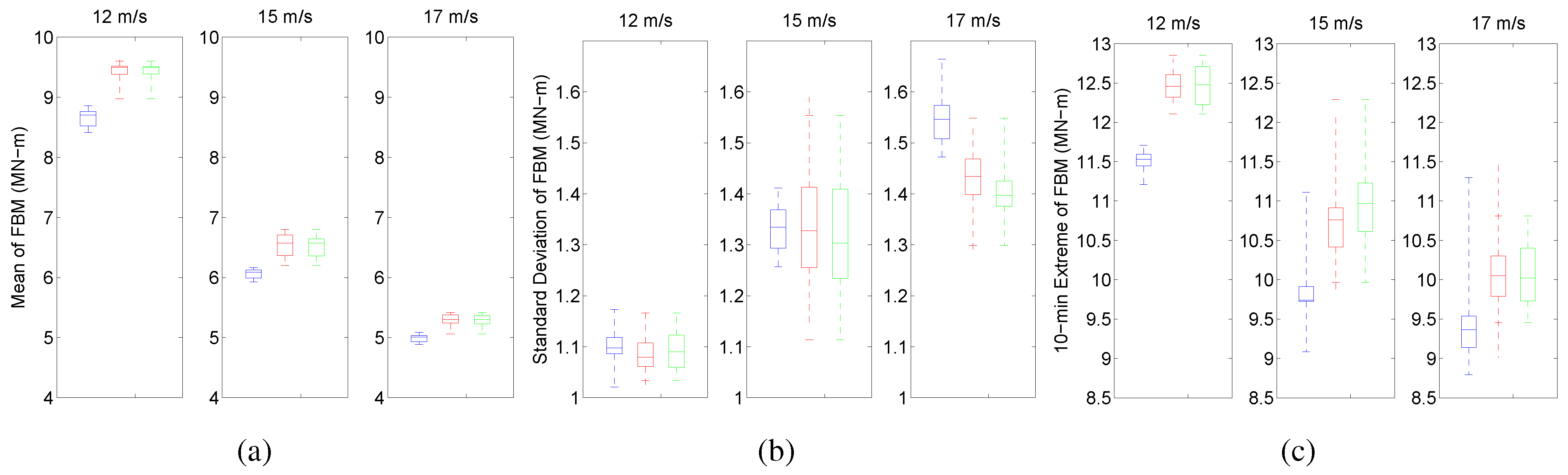
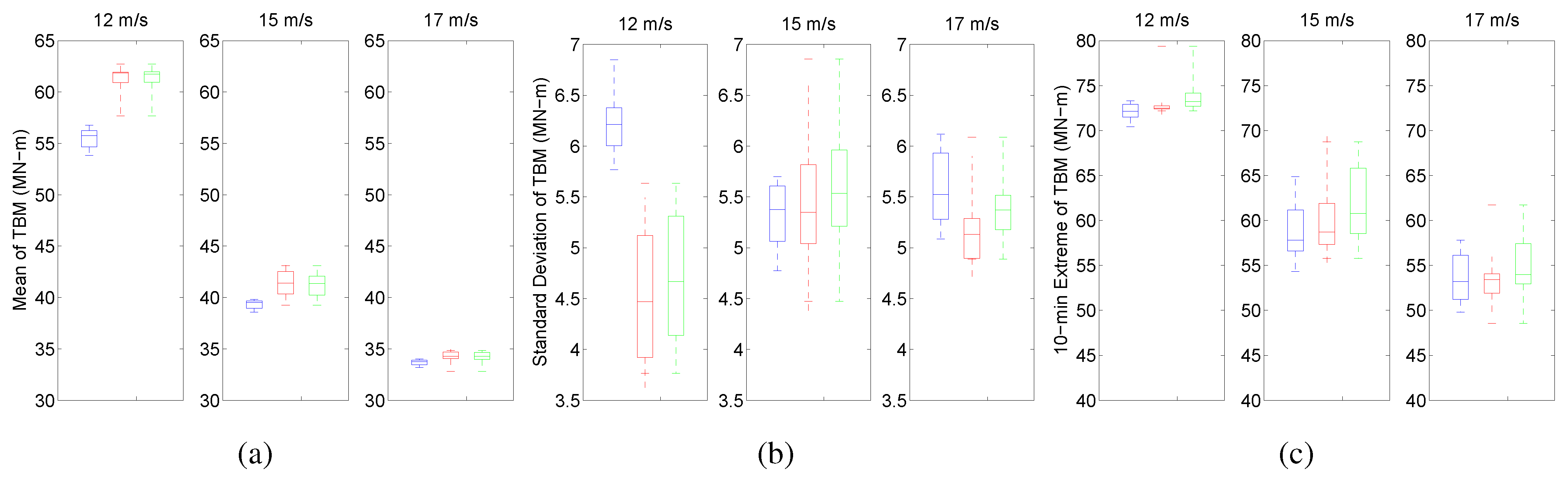
4.1. Turbine Load Statistics

We study turbine load statistics for inflow fields generated by different simulation techniques. These inflow fields are based on three different simulation models: LES, LES with FIT, and TurbSim; and three different ten-minute mean hub-height wind speeds: 12 m/s, 15 m/s, and 17 m/s. (Note that, in this part of the study that involves comparing of turbine load statistics for LES and stochastic simulation, the LES cases were run first and led to hub-height mean wind speeds of 12 m/s, 15 m/s and 17 m/s; then, stochastic simulation for the inflow for these same wind speeds was carried out. This is in contrast to the first part of this study on spatio-temporal resolution where controlled stochastic simulation at wind speeds of 12 m/s, 15 m/s, and 18 m/s were used.) We are interested in the ten-minute extreme, the ten-minute mean, and the standard deviation for the two different turbine loads (FBM and TBM). A total of fifteen simulations were used for the turbine load calculations with each of the inflow fields. The results of these simulations are represented in box plots, also referred to as box-whisker diagrams [29]. Quartiles that represent the 25% (lower quartile), 50% (median), and the 75% (upper quartile) are extracted from the data set; these quartiles form the box, while the whiskers indicate the range from minimum to maximum. The box-whisker plots for FBM and TBM illustrated in Figure 7 and Figure 8, respectively, identify the quartiles as well as maximum and minimum values of the relevant statistic (mean, standard deviation, or ten-minute maximum) from 15 realizations. Each figure summarizes statistics for the three inflow options (TurbSim, LES, LES + FIT) and the three wind speeds. The blue (left) box represents the TurbSim case; the red (center) box represents the LES case; and the green (right) box represents the case for LES inflow with fractal interpolation.

The loads are seen to have higher standard deviations with increasing wind speed. Ten-minute extreme loads and mean values for the two loads and for the different inflow simulation options suggest that inflow conditions associated with the hub-height wind speed of 12 m/s bring about the largest loads. These results are understandable since turbine loads generally decrease as wind speeds exceed the rated wind speed due to pitch control actions. In the following discussions, we focus only on loads from inflow fields with a hub-height mean wind speed of 12 m/s.

Figure 7. Box-whisker plots summarizing ensemble statistics for FBM based on 15 simulations: mean (a); standard deviation (b); ten-minute maximum (c). Results presented are for TurbSim (blue), LES (red), and LES + FIT (green).

Figure 7. Box-whisker plots summarizing ensemble statistics for FBM based on 15 simulations: mean (a); standard deviation (b); ten-minute maximum (c). Results presented are for TurbSim (blue), LES (red), and LES + FIT (green).

Figure 8. Box-whisker plots summarizing ensemble statistics for TBM based on 15 simulations: mean (a); standard deviation (b); ten-minute maximum (c). Results presented are for TurbSim (blue), LES (red), and LES + FIT (green).

Figure 8. Box-whisker plots summarizing ensemble statistics for TBM based on 15 simulations: mean (a); standard deviation (b); ten-minute maximum (c). Results presented are for TurbSim (blue), LES (red), and LES + FIT (green).

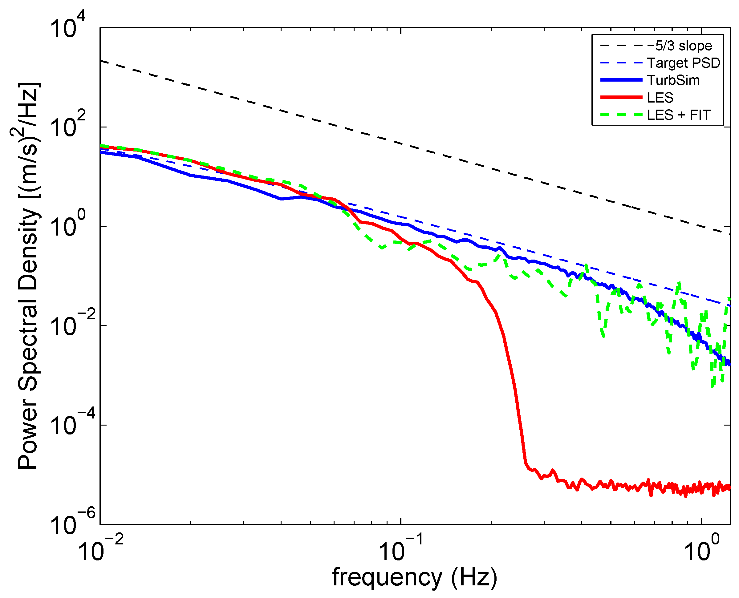
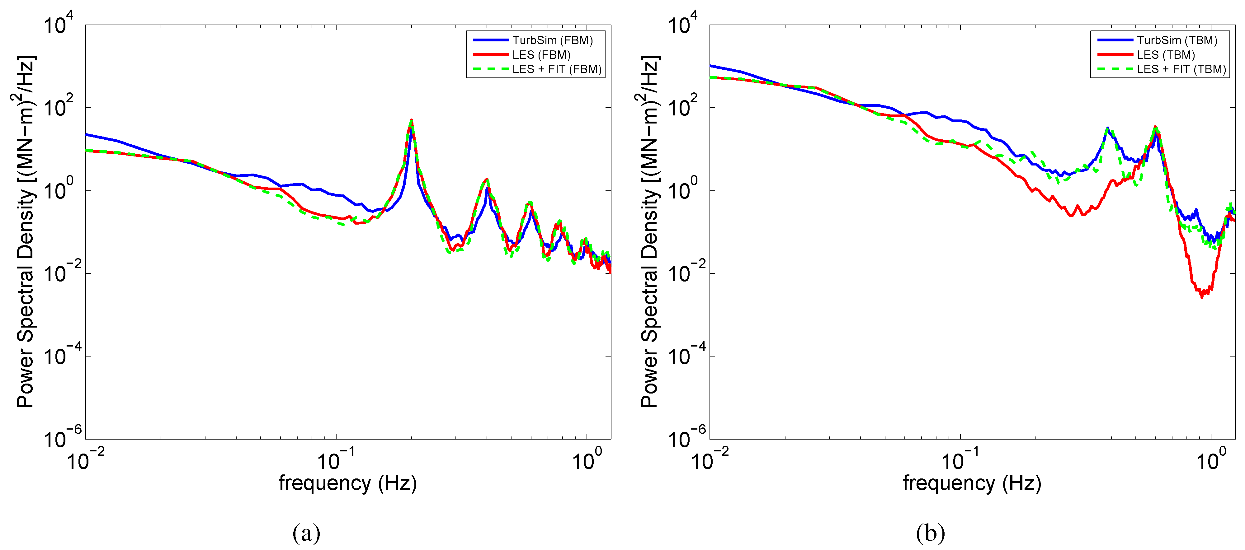
4.2. Power Spectral Density Functions of Turbine Loads

Power spectral density (PSD) estimates of turbine loads that result from inflow turbulence generated by TurbSim, LES, and LES with FIT are plotted in Figure 9. On studying the FBM power spectra in Figure 9, it may be seen that although there is some energy loss in the power spectra for LES at low frequencies, the dominant (1P) spectral peak matches that from the PSD for TurbSim quite well, even without applying fractal interpolation. All the spectral peaks shown (such as at 1P, 2P, 3P, etc.) are quite close for all the inflow simulation options. The benefit of applying FIT to LES-generated flow fields is not great.

Figure 9. Power spectral density function for FBM (a) and TBM (b) for different inflow simulation options with a hub-height ten-minute mean wind speed of 12 m/s.

Figure 9. Power spectral density function for FBM (a) and TBM (b) for different inflow simulation options with a hub-height ten-minute mean wind speed of 12 m/s.

While the blade loads under inflow turbulence generated by LES, even without FIT, preserved the important peaks in the power spectra reasonably well, the TBM power spectrum with LES inflow misses the peak at the natural frequency of the first tower fore-aft bending mode as can be seen in Figure 9. Since this first spectral peak makes an important contribution to the overall energy content, this deficit can lead to errors in tower load estimation. However, fractal interpolation recovers much of the missing energy between 0.4 Hz and 0.8 Hz, as can be seen in the power spectrum for LES with FIT. Interestingly, Figure 9 shows that with the exception of the tower first mode, many of the other spectral peaks are preserved quite well—for instance, the FBM power spectra at all frequencies and the TBM power spectrum at 3P are very similar for TurbSim and for LES despite the missing energy at high frequencies in the inflow turbulence with LES. The reason for the good matches is because at all these well-matched peaks, rotational sampling of the inflow wind assures adequate energy is transferred to the rotor thrust and the loads. It is only at frequencies that do not align well with rotationally sampled inflow, such as is the case with the tower fundamental mode, where one finds deficient spectral peaks for LES compared to TurbSim and LES with FIT.

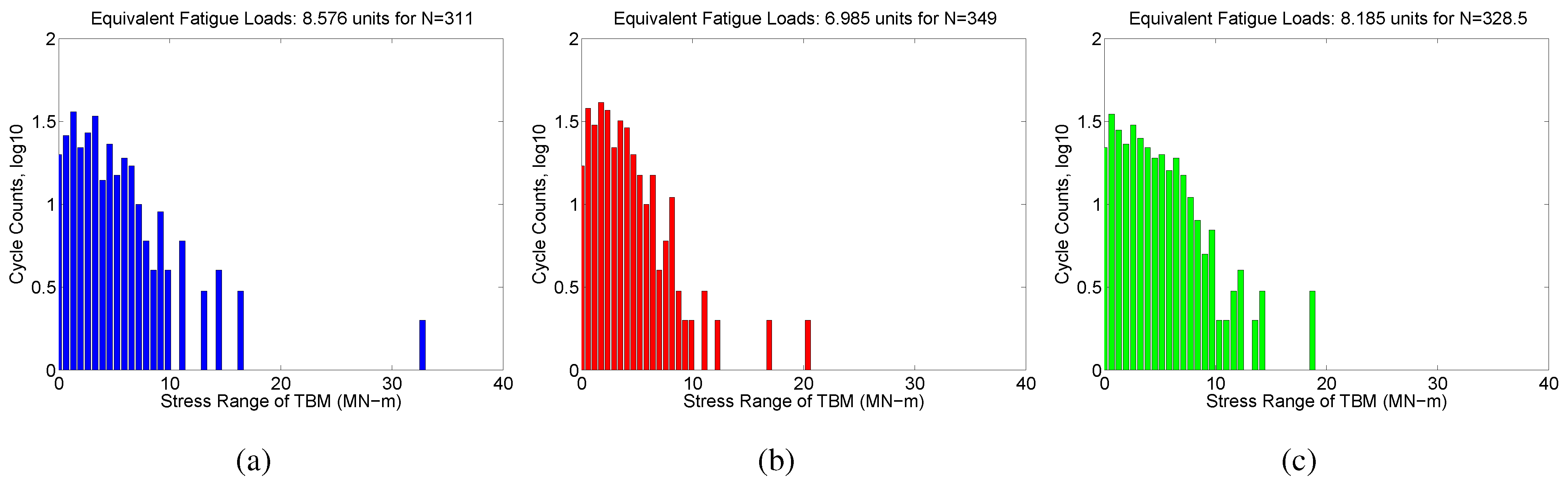
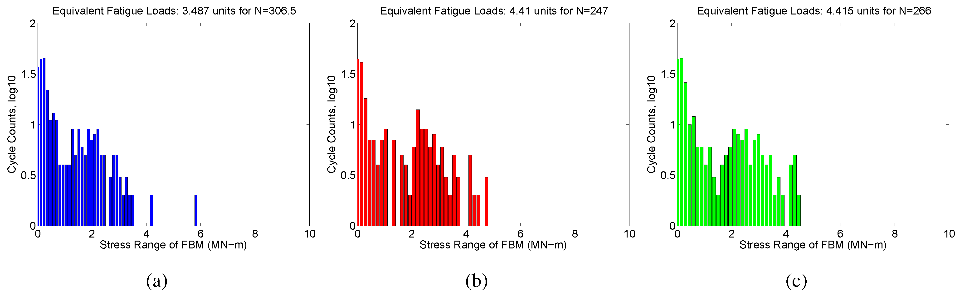
4.3. Fatigue Load Estimation

Stress range histograms can be established from time series of wind turbine loads by various means, including use of the rainflow cycle-counting algorithm [30], which is a commonly employed method for counting the number of cycles in an irregular load or stress time series. To obtain equivalent fatigue load (EFL) estimates for the wind turbine, Wöhler exponents equal to 3 and 10, respectively, are assumed for the steel tower (i.e., for TBM) and for the blades composed of fiber composite material (i.e., for FBM).

From each of the 15 simulated time series, load cycles were counted using the rainflow cycle-counting algorithm. The resulting stress cycles were binned into histograms and the equivalent fatigue load (EFL) and effective number of cycles (N) were also computed. Figure 10 and Figure 11 show fatigue stress range histograms of FBM and TBM, respectively.

Figure 10. Fatigue load range histograms based on 15 simulations for FBM (wind speed = 12 m/s): TurbSim (a); LES (b); LES + FIT (c).

Figure 10. Fatigue load range histograms based on 15 simulations for FBM (wind speed = 12 m/s): TurbSim (a); LES (b); LES + FIT (c).

Figure 11. Fatigue stress range histograms based on 15 simulations for TBM (wind speed = 12 m/s): TurbSim (a); LES (b); LES + FIT (c).

Figure 11. Fatigue stress range histograms based on 15 simulations for TBM (wind speed = 12 m/s): TurbSim (a); LES (b); LES + FIT (c).

Load range histograms based on LES flows are slightly lacking in some of the stress cycle bins compared to the those from the TurbSim flows. It is evident that fractal interpolation helps by filling in some of the missing cycles; this is more obvious for the TBM histogram. The TBM EFL estimate for LES inflow was significantly smaller than the EFL value based on TurbSim inflow before FIT was applied. After fractal interpolation, the equivalent fatigue load and damage were comparable with that from TurbSim inflow.

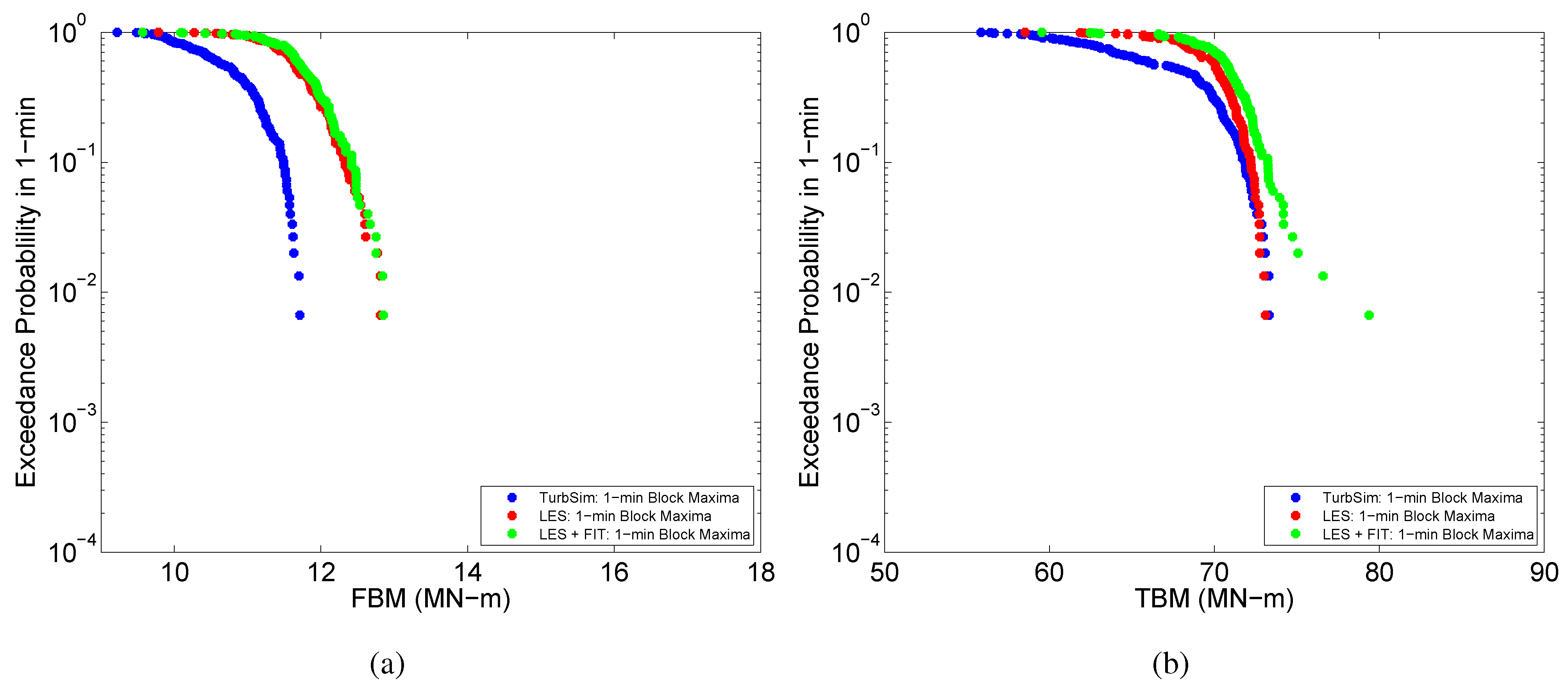
4.4. Load Probability Distributions

The International Electrotechnical Commission (IEC) standard [1] for the design of wind turbines includes a load case (for an ultimate limit state) that requires estimation of a 50-year return period load. In order to estimate this rare load from a limited number of simulations, one needs to use statistical extrapolation to predict this rare long-term load. Design Load Case (DLC) 1.1 in the IEC standard requires inflow turbulence under near-neutral atmospheric conditions and with specified turbulence intensity values that should be simulated with a normal turbulence model (NTM). The ten-minute average hub-height wind speed is treated as a single random variable representing the environment. In addition, to obtain loads for addressing DLC 1.1, the IEC standard requires one to perform aeroelastic simulations for the entire power-producing wind speed range from cut-in to cut-out. In this study, our simulations are limited to three specific wind speeds since the objective of this study was only to evaluate alternate inflow simulation methods. As a result, we only compute so-called “short-term” load distributions for the wind speeds studied; we do not attempt a full long-term load extrapolation.

In order to predict short-term load extremes from ten-minute time series, one can use the peak-over-threshold (POT) method, extract global (ten-minute) maxima, or extract block maxima (maxima over fixed intervals shorter than ten minutes). Agarwal [31] demonstrated that the three alternative extreme models—peak-over-threshold (POT), global maxima, and block maxima—all give comparable load distributions if a sufficient number of simulations are available to establish the distribution tails. The present study is based on a limited number of simulations; hence, we use one-minute block maxima to define our extreme load statistics. Under the assumption that these one-minute maxima are independent of each other, the short-term ten-minute maximum (L) distribution may be obtained for any wind speed $V=v$ from the short-term block maxima ($L_{block}$). In terms of the probability of exceedance of any load level, l, the short-term global maxima distribution may be expressed as follows:

$$P(\left.L>l\right|V=v)=1-{[1-P(\left.L_{block}>l\right|V=v)]}^n$$

(4)

Accounting for the different values of V, the long-term distribution on L can be obtained as follows:

$$P(L>l)=\underset{V_{in}}{\overset{V_{out}}{\int }}P(L>l\left|V=v)f_V\left(v\right)dv\right.$$

(5)

where $f_V\left(v\right)$ is the wind speed probability density function, which is usually taken to be a Weibull density function (of which, the Rayleigh distribution is a special case).

Figure 12 shows the short-term distribution for FBM and TBM loads. For the FBM loads, fractal interpolation leads to no change in the load distribution obtained using LES. The difference between LES and TurbSim predictions of the 80th percentile ten-minute maximum value (or, equivalently, of the load associated with a 0.022 non-exceedance probability in 1 min) is approximately $10\%$ for this load. For the TBM loads, the LES distribution matches that from TurbSim while fractal interpolation introduces a deviation in the distribution tail. It appears that possibly excessive high-frequency energy introduced by FIT causes larger loads in a few simulations that directly influences the distribution tails. Note, however, that the short-term loads distributions presented here are based only on a limited number of simulations (and uncertainty is especially an issue for rare fractiles and with small sample sizes); additional simulations might be warranted to establish stable extreme distribution tails.

Figure 12. Short-term probability distributions of wind turbine loads for a wind speed of 12 m/s for FBM (a) and TBM (b).

Figure 12. Short-term probability distributions of wind turbine loads for a wind speed of 12 m/s for FBM (a) and TBM (b).

5. Conclusions

Findings from this study suggest that in inflow wind field simulations, a grid spacing around one-tenth of the rotor diameter ($\approx 10$ m) and 1 Hz inflow data (temporal filtering) may be adequate for loads studies. In particular, such space-time resolution may be justified in flow field generation using either stochastic simulation or large-eddy simulation (LES). An LES computational framework was defined with this consideration.

Turbine loads under inflow turbulence generated by different simulation techniques (LES versus stochastic) were compared. Inflow turbulence for a neutrally stratified boundary layer generated by conventional stochastic simulation, large-eddy simulation, and large-eddy simulation with fractal interpolation was considered. Load statistics were studied to understand the characteristics of turbine loads at different hub-height wind speeds. The hub-height wind speed of 12 m/s had the largest loads compared to the wind speeds of 15 m/s or 17 m/s. Fractal interpolation was helpful for recovering energy deficit at high frequencies in large-eddy simulations. Fatigue loads and stress range histograms were also studied; again fractal interpolation improved the stress cycle histograms from LES versus stochastic simulation especially for tower loads. Short-term load distributions of turbine loads were studied using 1-min block maxima; these distributions from stochastic simulation and LES were reasonably consistent with each other.

Based on the various turbine load studies conducted, it is concluded that large-eddy simulations with fractal interpolation can generate turbine loads that are comparable with the stochastic simulation results. For fatigue and ultimate limit states, LES with FIT is an attractive alternative to stochastic simulation. Having demonstrated its effectiveness as has been done here, additional studies are being carried out where LES with FIT is being employed to assess loads on turbines in the stable boundary layer where stochastic simulation is no longer possible.

References

1. International Electrotechnical Commission. Wind Turbines—Part 1: Design Requirements, 3rd ed.; IEC-61400-1; International Electrotechnical Commission: Geneva, Switzerland, 2005. [Google Scholar]
2. Veers, P. Three-Dimensional Wind Simulation; Technical Report SAND88-0152; Sandia National Laboratory: Albuquerque, NM, USA, 1988. [Google Scholar]
3. Mücke, T.; Kleinhans, D.; Peinke, J. Atmospheric turbulence and its influence on the alternating loads on wind turbines. Wind Energy 2011, 14, 301–316. [Google Scholar] [CrossRef]
4. Jonkman, B. TurbSim User’s Guide: Version 1.50; Technical Report NREL/TP-500-46198; National Renewable Energy Laboratory: Golden, CO, USA, 2009. [Google Scholar]
5. Kaimal, J.C.; Wyngaard, J.C.; Izumi, Y.; Coté, O.R. Spectral characteristics of surface-layer turbulence. Q. J. R. Meteorol. Soc. 1972, 98, 563–589. [Google Scholar] [CrossRef]
6. Jonkman, J.; Butterfield, S.; Musial, W.; Scott, G. Definition of a 5 MW Reference Wind Turbine for Offshore System Development; Technical Report NREL/TP-500-38060; National Renewable Energy Laboratory: Golden, CO, USA, 2007. [Google Scholar]
7. Jonkman, J.; Buhl, M. FAST User’s Guide; Technical Report NREL/EL-500-38230; National Renewable Energy Laboratory: Golden, CO, USA, 2005. [Google Scholar]
8. Hansen, M. Aerodynamics of Wind Turbines, 2nd ed.; Earthscan Publications Ltd.: London, UK, 2008. [Google Scholar]
9. Fogle, J.; Agarwal, P.; Manuel, L. Towards an improved understanding of statistical extrapolation for wind turbine extreme loads. Wind Energy 2008, 11, 613–635. [Google Scholar] [CrossRef]
10. Kelley, N.; Osgood, R.; Bialasiewicz, J.; Jakubowski, A. Using wavelet analysis to assess turbulence/rotor interactions. Wind Energy 2000, 3, 121–134. [Google Scholar] [CrossRef]
11. Pope, S.B. Turbulent Flows; Cambridge University Press: Cambridge, UK, 2000. [Google Scholar]
12. Sagaut, P. Large Eddy Simulations for Incompressible Flows; Springer-Verlag: Berlin, Germany, 2001; pp. 1–426. [Google Scholar]
13. Geurts, B.J. Elements of Direct and Large-Eddy Simulation; Edwards: Philadelphia, PA, USA, 2003; pp. 1–329. [Google Scholar]
14. Basu, S.; Vinuesa, J.F.; Swift, A. Dynamic LES modeling of a diurnal cycle. J. Appl. Meteorol. Climatol. 2008, 47, 1156–1174. [Google Scholar] [CrossRef]
15. Nieuwstadt, F.T.M.; Mason, P.J.; Moeng, C.H.; Schumann, U. Large-eddy simulation of the convective boundary layer: A comparison of four computer codes. In Turbulent Shear Flows 8; Durst, F., Friedrich, R., Launder, B.E., Schmidt, F.W., Schumann, U., Whitelaw, J.H., Eds.; Springer: Berlin, Germany, 1991; pp. 343–367. [Google Scholar]
16. Andrén, A.; Brown, A.R.; Graf, J.; Mason, P.J.; Moeng, C.H.; Nieuwstadt, F.T.M.; Schumann, U. Large-eddy simulation of a neutrally stratified boundary layer: A comparison of four computer codes. Q. J. R. Meteorol. Soc. 1994, 120, 1457–1484. [Google Scholar] [CrossRef] [Green Version]
17. Beare, R.J.; Macvean, M.K.; Coauthors. An Intercomparison of large-eddy simulations of the stable boundary layer. Bound. Layer Meteorol. 2006, 118, 247–272. [Google Scholar] [CrossRef]
18. Uchida, T.; Ohya, Y. Micro-siting technique for wind turbine generators by using large-eddy simulation. J. Wind Energy Ind. Aerodyn. 2008, 96, 2121–2138. [Google Scholar] [CrossRef]
19. Calaf, M.; Meneveau, C.; Meyers, J. Large eddy simulation study of fully developed wind-turbine array boundary layers. Phys. Fluids 2010, 22, 015110. [Google Scholar] [CrossRef]
20. Bechmann, A.; Sørensen, N.N. Hybrid RANS/LES applied to complex terrain. Wind Energy 2011, 14, 225–237. [Google Scholar] [CrossRef]
21. Bechmann, A.; Sørensen, N.N.; Berg, J.; Mann, J.; Réthoré, P.E. The bolund experiment, Part II: Blind comparison of microscale flow models. Bound. Layer Meteorol. 2011, 141, 245–271. [Google Scholar] [CrossRef]
22. Wu, Y.T.; Porté-Agel, F. Large-Eddy Simulation of Wind-Turbine Wakes: Evaluation of Turbine Parametrisations. Bound. Layer Meteorol. 2011, 138, 345–366. [Google Scholar] [CrossRef]
23. Basu, S.; Porté-Agel, F. Large-eddy simulation of stably stratified atmospheric boundary layer turbulence: A scale-dependent dynamic modeling approach. J. Atmos. Sci. 2006, 63, 2074–2091. [Google Scholar] [CrossRef]
24. Basu, S.; Porté-Agel, F.; Foufoula-Georgiou, E.; Vinuesa, J.F.; Pahlow, M. Revisiting the local scaling hypothesis in stably stratified atmospheric boundary layer turbulence: An integration of field and laboratory measurements with large-eddy simulations. Bound. Layer Meteorol. 2006, 119, 473–500. [Google Scholar] [CrossRef]
25. Anderson, W.C.; Basu, S.; Letchford, C.W. Comparison of dynamic subgrid-scale models for simulations of neutrally buoyant shear-driven atmospheric boundary layer flows. Environ. Fluid Mech. 2007, 7, 195–215. [Google Scholar] [CrossRef]
26. Vinuesa, J.F.; Basu, S.; Galmarini, S. The diurnal evolution of 222Rn and its progeny in the atmospheric boundary layer during the Wangara experiment. Atmos. Chem. Phys. 2007, 7, 5003–5019. [Google Scholar] [CrossRef]
27. Basu, S.; Holtslag, A.A.M.; Bosveld, F.C. GABLS3 LES Intercomparison Study. In Proceedings of ECMWF/GABLS Workshop on “Diurnal Cycles and the Stable Atmospheric Boundary Layer”; UK, 7–10 November 2011, European Centre for Medium-Range Weather Forecasts (ECMWF): Reading, UK; World Climate Research Programme (WCRP): Geneva, Switzerland, 2011; pp. 75–82. [Google Scholar]
28. Basu, S.; Foufoula-Georgiou, E.; F. Porté-Agel, F. Synthetic turbulence, fractal interpolation, and large-eddy simulation. Phys. Rev. E 2004, 70, 026310. [Google Scholar] [CrossRef] [PubMed]
29. Tukey, J. Extrapolatory Data Analysis; Addison-Wesley: New York, NY, USA, 1977. [Google Scholar]
30. American Society for Testing and Materials Standards. Standard Practices for Cycle Counting in Fatigue Analysis; E1049-85; ASTM International: West Conshohocken, PA, USA, 1985. [Google Scholar]
31. Agarwal, P. Structural Reliability of Offshore Wind Turbines. Ph.D. Dissertation, University of Texas at Austin, Austin, TX, USA, 2008. [Google Scholar]