Study on the Development of an Optimal Heat Supply Control Algorithm for Group Energy Apartment Buildings According to the Variation of Outdoor Air Temperature

Abstract

In the present study, we have developed an optimal heat supply algorithm which minimizes the heat loss through the distribution pipe line in a group energy apartment. Heating load variation of a group energy apartment building according to the outdoor air temperature was predicted by a correlation obtained from calorimetry measurements of all households in the apartment building. Supply water temperature and mass flow rate were simultaneously controlled to minimize the heat loss rate through the distribution pipe line. A group heating apartment building located in Hwaseong city, Korea, which has 1473 households, was selected as the object building to test the present heat supply algorithm. Compared to the original heat supply system, the present system adopting the proposed control algorithm reduced the heat loss rate by 10.4%.

1. Introduction

Research on group energy heating systems has been conducted continuously in Europe over the years as well as in the U.S.A and Japan. Group energy heating is district heating for apartment building containing various households. Research on district heating is needed to meet individual household heating needs while minimizing heat losses.

Bøhm et al. [1] research includes energy and exergy analysis of group energy heat sources and heat using facilities. Stevanovic et al. [2] researched a group energy heating system using non-used energy and renewable energy, Wu et al. [3,4,5,6] studied the economic feasibility of group energy heating system and improvement of policies and regulations.

Bøhm et al. [1] analyzed group apartment building energy usage and pump efficiency and heat exchanger efficiency in the Copenhagen (Denmark) area, while Knutsson et al. [7] developed a simulation method for energy analysis according to fuel usage in local heating. Shimoda et al. [8] proved the benefits of local heating and cooling systems through energy simulation, considering design parameters and operating condition. Lin et al. [9] presented an optimization method and modeling of group energy heating system pipeline and effect of supply water temperature and return water temperature of local heating and cooling system in China according to energy usage. Larsen et al. [10] conducted research on heat source facility system performance improvement and optimized control and also conducted simulation analysis of local heating and cooling system pipeline for optimization of group energy heating system supply water temperature, and compared German method and Danish method of group energy heating system modeling analysis [11]. Bojic et al. [12] tried to improve system performance by developing an optimizing program for efficient heat supply distribution in group energy heating systems. Nielsen et al. [13] suggested a mathematical modeling method of group energy system energy consumption rate according to Denmark climate change (grey-box modeling).

There are studies on group energy heating system modeling and performance such as the research conducted by Holmgren et al. [14], which suggested the environmental effects of incineration facilities including CO₂ emissions and economical group energy heating system usage through simultaneous heat consumption in industrial estates.

Henning et al. [15] optimized a Swedish group energy heating system of combined heat and power plant which uses various fuels, with the MODEST simulation method. Gabrielaitinene et al. [16] compared simulated results of medium temperature water supply water temperature and return water temperature in a Naestved (Denmark) area group energy heating system with experimental results. The study reported slight differences in experimental and simulated results in long distance pipelines with large numbers of joints and bend pipes. Stevanovic et al. [2] suggested a numerical method for analysis of the energy saving effects of pump operations in a complex group energy heating system pipeline through prediction of supply water temperature in the steady state.

Lianzhong et al. [17] studied the optimal operation of group energy heating systems for energy savings. Wu et al. [3] suggested a method for deducing and optimizing the economic and environmental effects of a heat & power plant based group energy heating system using an energy equilibrium model method. Dotzauer et al. [4] suggested a long term proposal over a month through optimal modeling and simulation methods to meet basic heat consumption needs according to group energy heating system operation mode, while minimizing operational costs. Dotzauer [5] also suggested a heat load prediction model according to outdoor temperature changes for optimal operation of a local heating system, and Heller [6] suggested a heat load estimation model for optimal group energy composition. Langendries [18] proved maintenance of lowest return water temperature as the crucial operating factor in reducing group energy heat losses. However, among group energy heat supply system studies, there is no research conducted on optimal heat supply system that meets consumer needs and minimizes pipeline heat loss while supply water temperature and supply water rate are both varied.

In the studied Korean group energy apartment building heating system, supply water temperature and supply water rates of the consumer side are varied by the heat exchange between the primary pipeline and the secondary pipeline, which can be expressed as an empirical equation, according to the season and the outdoor temperature, but this empirical method results in increased supply water temperature and return water temperature, that increase heat losses in the heat supply pipeline and return pipeline. In this study, a variable supply water rate, variable supply water temperature optimal control algorithm is proposed to minimize the pipeline heat loss in a group energy heating system that supplies the required heat to each house hold according to the change in weather.

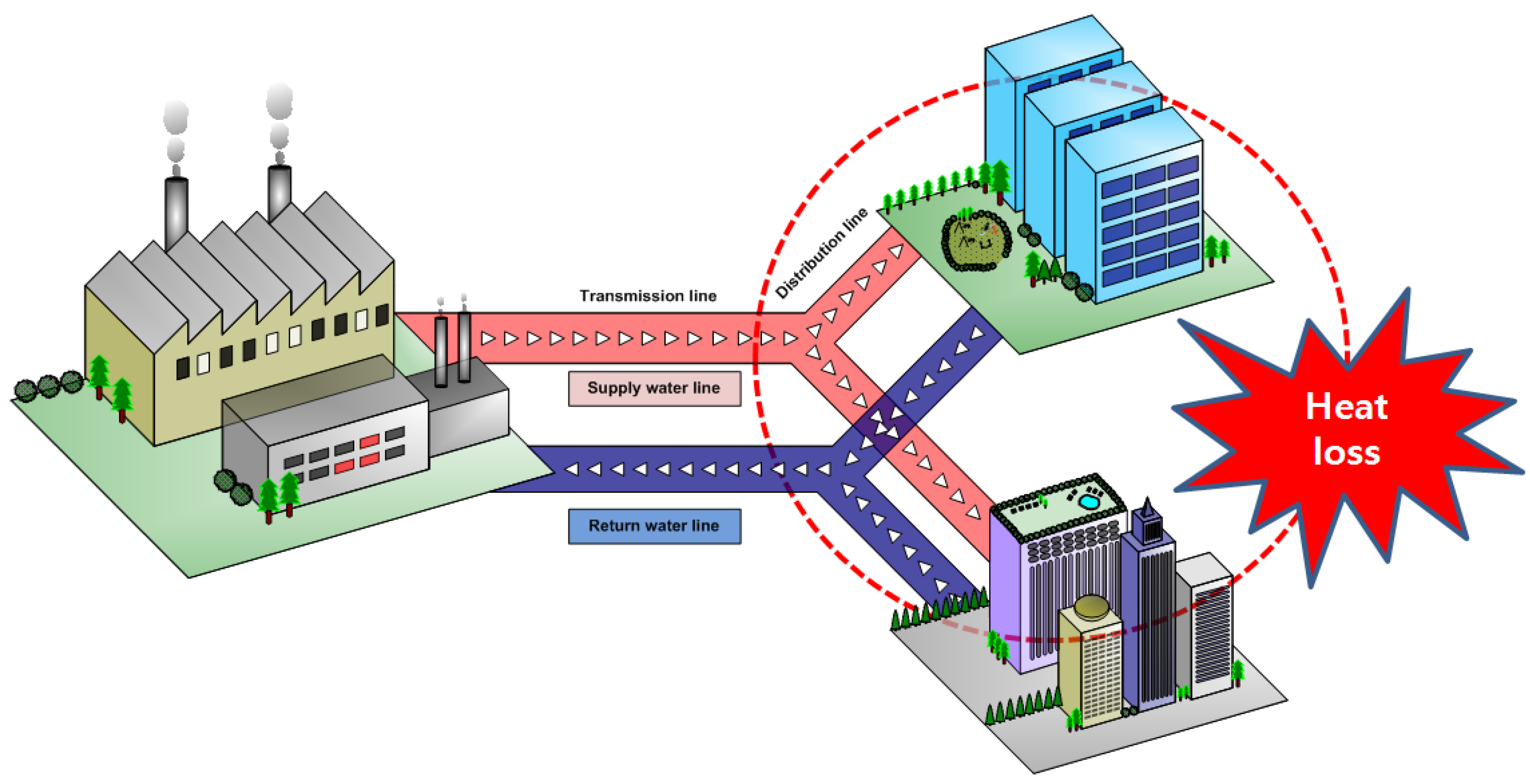
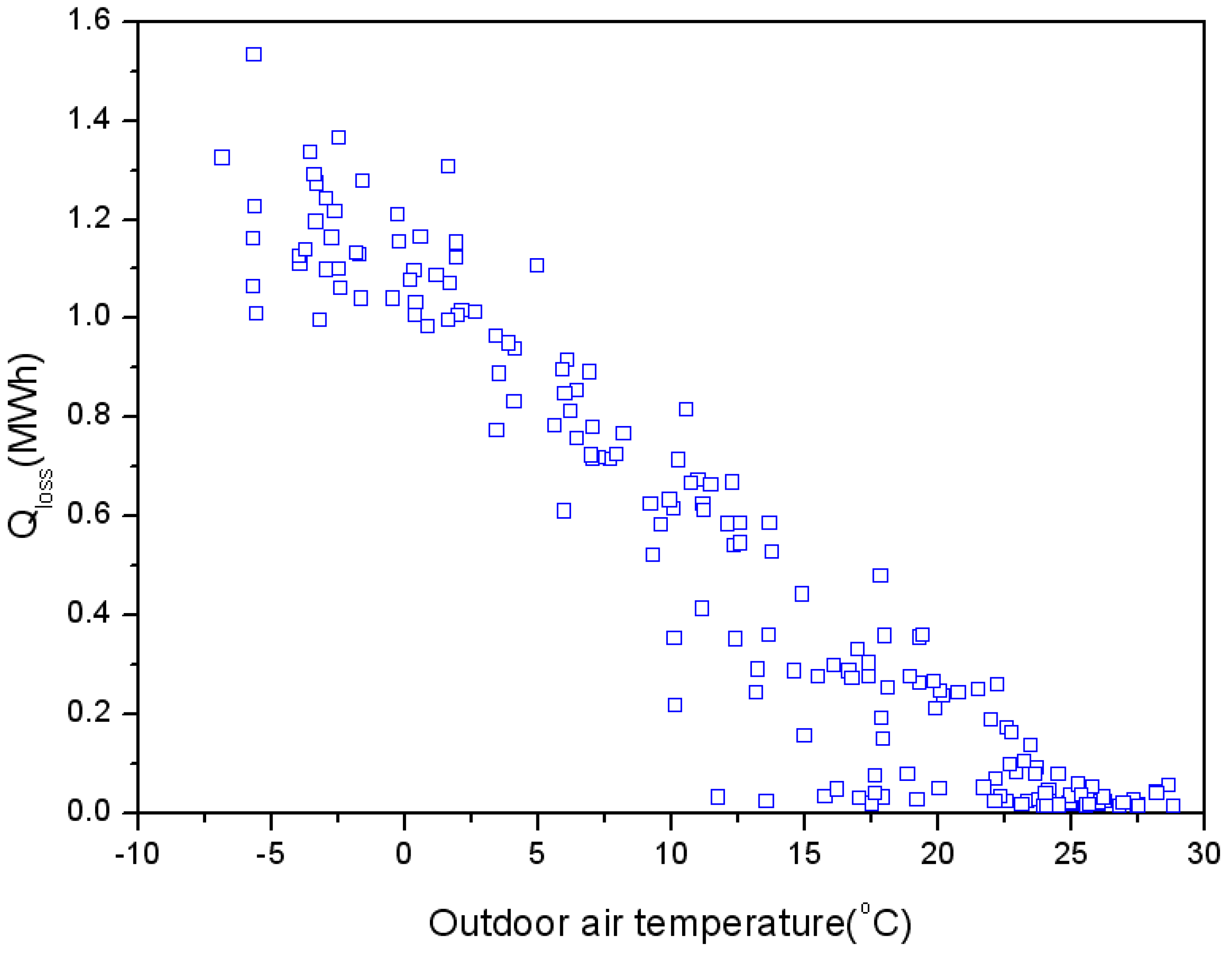
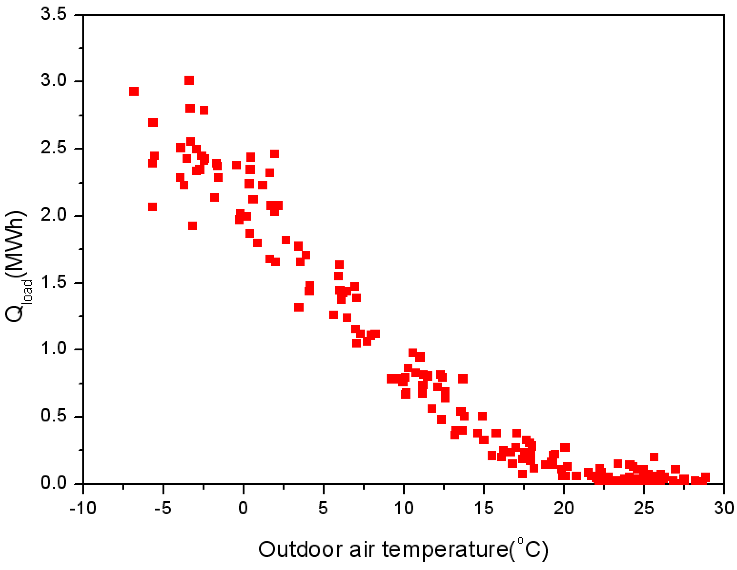
2. Analysis of Group Energy Apartment Building Heat Loss

A schematic of the studied Korean group energy heating system is shown in Figure 1. Heat is generated by the district heating corporation using fuel. Heat is transferred to the heat consuming facility via a heat transfer facility.

Figure 1. Schematic diagram of district heating system.

Figure 1. Schematic diagram of district heating system.

Apartment buildings, shopping centers and public buildings are such heat consuming facilities. District heating water produced by the heat generating facility is pressurized and supplied to the consumer’s (secondary) machinery room through a heat supply line in the heat supply system. The machinery room transfers heat to each consumer by a heat exchanger. Group energy transmission line is the water line connecting heat generating facility and apartment building machinery room. Group energy distribution line is the water line connecting apartment building machinery room and individual households in apartment building. Thus heat is generated at heat generating facility and transferred through transmission line and then distribution line to reach individual households.

In Korea, heat is transferred at a mandatory pressure and temperature of 16 bar and 120 °C, respectively [19]. In this study, apartment building D located in Gyeonggi-do Hwaseong city (Korea) was chosen as the target group energy heat supply apartment building. The variations of the heat loss rates in the heat supply line and the return line were investigated according to the variation in the outdoor temperature. The data provided a data base for development of an optimal heat supply control algorithm. The target apartment building specifications are provided in Table 1.

Table 1. Specifications of model group energy apartment for optimal heat supply control.

Item	Specifications
Object building	Apartment building
Number of households	1473
Period	2008.01.01~2008.12.31
Location	Hwaseong city, Gyeonggi-do, Korea
Heating source	District heating

Table 1. Specifications of model group energy apartment for optimal heat supply control.

Item	Specifications
Object building	Apartment building
Number of households	1473
Period	2008.01.01~2008.12.31
Location	Hwaseong city, Gyeonggi-do, Korea
Heating source	District heating

In this study, the supply water temperature and supply water flow rate were automatically controlled to provide each heat consuming house with sufficient heat at the lowest supply water temperature and return water temperature. An optimal heat supply control algorithm was developed to minimize the heat losses in the distribution line.

Experimental Data for Numerical Analysis

Figure 2 shows the variations of supply water temperature and return water temperature on the group energy apartment building supplier side (primary side), recorded for one year. The group energy supplier decides the supply water temperature and flow rate based on an empirical equation according to seasonal change.

Heat loss in the group energy transmission line is not considered in this study, because the objective of the research is to reduce heat losses in the distribution line.

The supply water temperature is constant around 110 °C from January to April, and in December, though it shows a slight variation according depending on the outdoor temperature. Between May and November, the supply water temperature varies between 90 °C and 100 °C according to the outdoor temperature. The return water temperature increases from 30 °C in summer to 45 °C in winter. But the return water temperature is not decided by the group energy heat supplier, but rather by the consumer side heat consumption rate, which varies according to outdoor temperature.

Supplier side and consumer side heat distribution lines exchange heat in the heat exchanger. Annual variations of supply and return water temperatures in the consumer side distribution line are shown in Figure 3. The figure shows that the supply water temperature is maintained at 53 °C during winter and 50 °C during spring, which is varied according to the outdoor temperature after May. But basis for determining the supply water temperature variation is vague. The variation of the supply water temperature seems to controlled by the empirical equation.

Figure 2. Annual variation of supply and return water temperatures of group energy primary side (supplier side) of the model apartment.

Figure 2. Annual variation of supply and return water temperatures of group energy primary side (supplier side) of the model apartment.

Figure 3. Annual variation of supply and return water temperatures of group energy secondary side (consumer side) of the model apartment.

Figure 3. Annual variation of supply and return water temperatures of group energy secondary side (consumer side) of the model apartment.

Figure 4 shows the annual variations of mass flow rates in the apartment building machinery transmission line and distribution line at the consumer side. How the temperature variation is determined is also difficult to define in this case. The temperature seems to be controlled by some empirical equation according to the outdoor temperature.

Figure 4. Annual variations of mass flow rates in the transmission and distribution lines of group energy supply system at the model group energy apartment.

Figure 4. Annual variations of mass flow rates in the transmission and distribution lines of group energy supply system at the model group energy apartment.

Figure 5 is a comparison between the heat supplied and the heat consumed in an apartment. The supplied heat is greater than the consumed heat, because of the heat loss that occurs in the distribution line as hot water is transmitted from the heat exchanger to individual homes.

Note that the amount of heat loss varies by season. The heat loss rate in the consumer side distribution line extracted from Figure 5 is shown in Figure 6.

Also annual variation of outdoor temperature is shown in Figure 6. Heat loss rate in the distribution line according to the outdoor air temperature variation is shown in Figure 7. The figure shows a linear increase of the heat loss rate (${\dot{Q}}_{loss}$) with the decrease of the outdoor temperature (T_air). Consumer side heat loss rate is the rate of heat loss as hot water is supplied from the heat exchanger to individual homes and is returned from the individual homes to the heat exchanger.

The objective of present study was to develop a heat supply control algorithm which minimizes the heat loss rate of the distribution line on the consumer side. Lowering the supply and return water temperatures to their minimums can minimize the heat loss rate, but the heat needed in apartments must be supplied as the supply and return water temperatures are lowered. A heat supply control algorithm is developed to minimize the supply and return water temperatures according to the outdoor temperature while meeting needs of heat consumption of individual homes.

Figure 5. Annual variations of heat supply and use rates of the model apartment.

Figure 5. Annual variations of heat supply and use rates of the model apartment.

Figure 6. Annual variation of heat loss rate of distribution line of the model apartment and annual variation of outdoor air temperature.

Figure 6. Annual variation of heat loss rate of distribution line of the model apartment and annual variation of outdoor air temperature.

Figure 7. Heat loss rate variation of distribution line at the model apartment with respect to outdoor air temperature.

Figure 7. Heat loss rate variation of distribution line at the model apartment with respect to outdoor air temperature.

Viewing the present study as an optimization problem, we have the following considerations:

• Constraint: Supply heat needed in individual homes according to outdoor temperature variation.
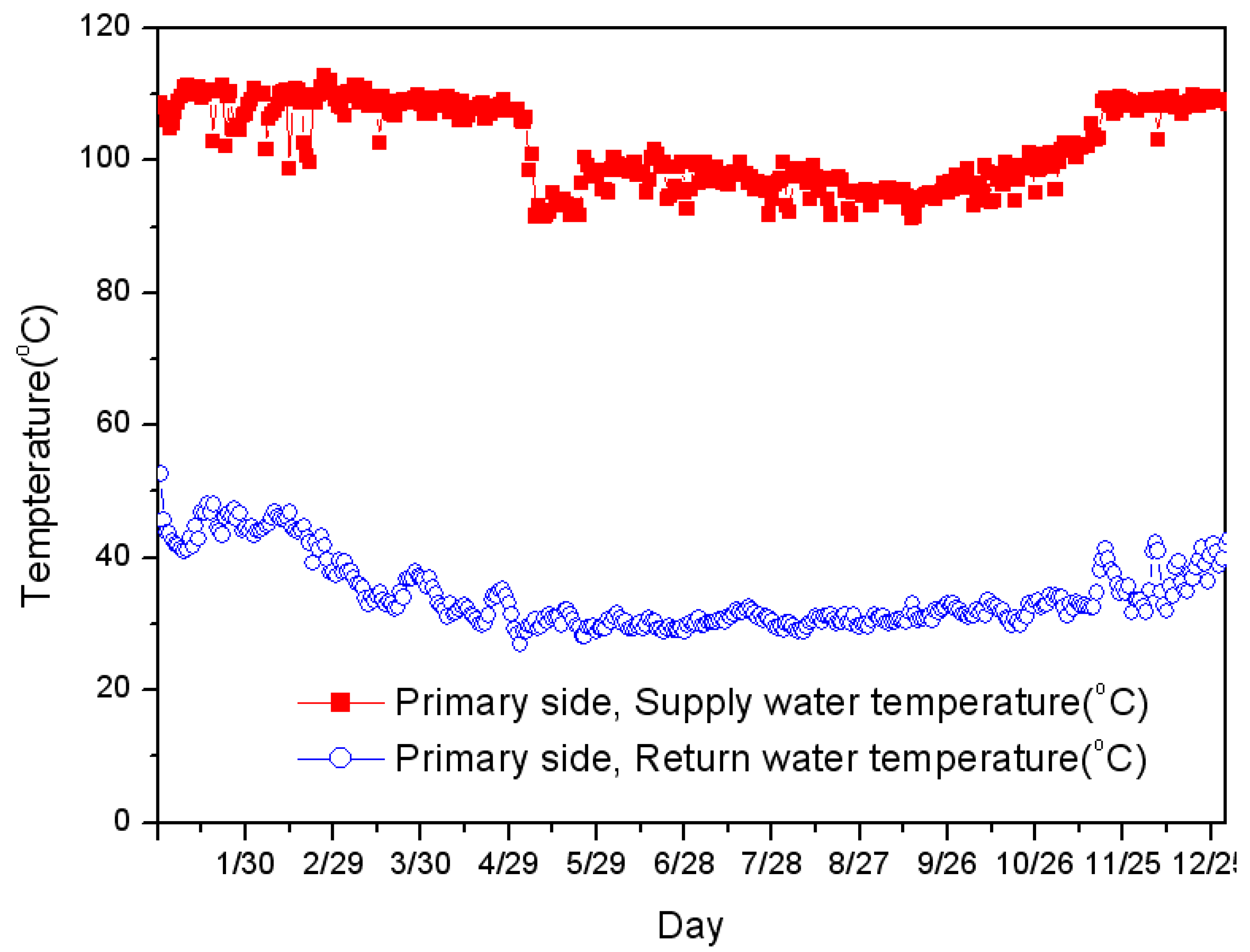
• Objective function: Determine supply water temperature and return water temperature that yield the lowest heat loss rate on the consumer side distribution line.

The heat loss rate in consumer side distribution line (${\dot{Q}}_{loss}$) can be expressed by the following equation, where T_s denotes the supply water temperature, T_air the outdoor temperature, (${\dot{m}}_S$) the supply water flow rate, and T_R the return water temperature:

$${\dot{Q}}_{loss}=f\left(T_S,T_{air},{\dot{m}}_s,T_R,\beta \right)$$

(1)

Here, β is the equivalent heat transfer coefficient between the heat supply distribution line and the outdoors. Meanwhile, the return water temperature can be expressed as:

$$T_R=g\left(T_S,T_{air},{\dot{m}}_s,\alpha \right)$$

(2)

Where α is the equivalent heat transfer coefficient between the floor and the room of a home in an apartment building. (The traditional heating system in Korea is the Ondol floor heating system [20].)

Substituting Equation (2) into Equation (1) yields:

$${\dot{Q}}_{loss}=f\left(T_S,T_{air},{\dot{m}}_s,\alpha ,\beta \right)$$

(3)

In this study, the heat loss rate in the consumer side distribution line was obtained from the difference between supplied heat and consumed heat in a standard group energy heat supply system. The optimal heat supply control algorithm for determining T_s and (${\dot{m}}_S$) that yields the minimal (${\dot{Q}}_{loss}$) in Equation (3) will be demonstrated.

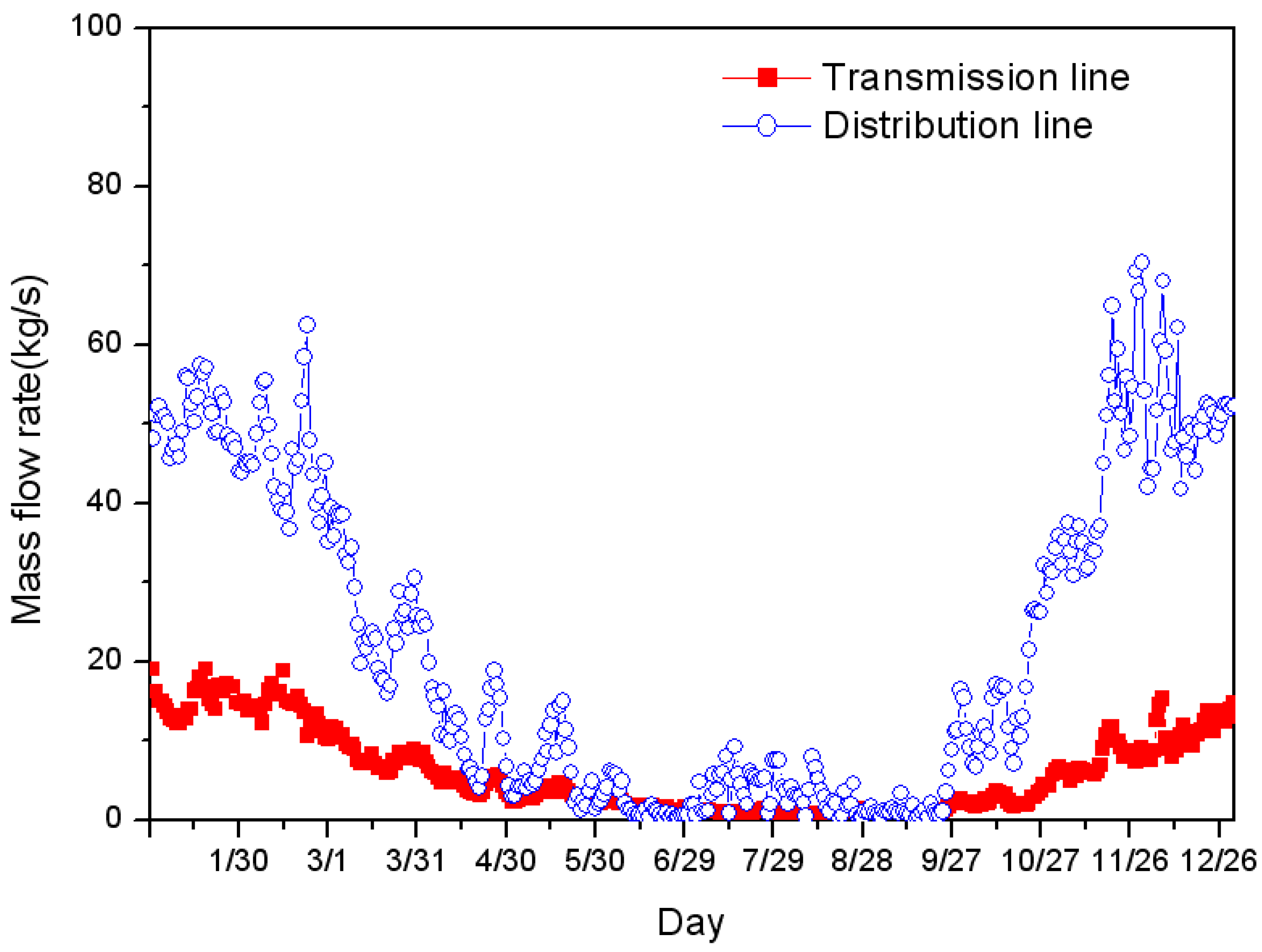
3. Analysis of Heat Loss in Heat Distribution Line of Target Group Energy Apartment Building

The optimal heat supply control algorithm varies the supply water temperature and supply water flow rate simultaneously according to the outdoor temperature, to minimize the heat loss rate in the heat supply distribution line while meeting the heat supply demands of the consumers. Figure 8 is a schematic diagram of the optimal heat supply control system with variable supply water temperature and variable mass flow rate.

Figure 8. Schematic diagram of optimal heat supply control algorithm that varies the supply water temperature and mass flow rate according to outdoor air temperature.

Figure 8. Schematic diagram of optimal heat supply control algorithm that varies the supply water temperature and mass flow rate according to outdoor air temperature.

The total heat load of a group energy apartment building can be expressed as a function of outdoor temperature and indoor average temperature:

$$\dot{Q}=f\left({\overline{T}}_{Room},T_{air}\right)$$

(4)

$${\dot{Q}}_h=\max \left({\dot{Q}}_h^1,{\dot{Q}}_h^2,{\dot{Q}}_h^3\right)$$

(5a)

$${\dot{Q}}_h^1=-102,380T+2,150,000$$

(5b)

$${\dot{Q}}_h^2=-47,272T+1,300,000$$

(5c)

$${\dot{Q}}_h^3=-10,000T+500,000$$

(5d)

Here, ${\overline{T}}_{Room}$ is the average indoor temperature of the individual apartments in the group apartment building, and T_air is the outdoor temperature. In this study, the indoor temperature is assumed as 22 °C from January to August and 23 °C from September to December. Heat load is a function of the outdoor temperature, as shown in Figure 9.

Figure 9. Variation of heating load of the model group energy apartment building according to outdoor air temperature.

Figure 9. Variation of heating load of the model group energy apartment building according to outdoor air temperature.

To develop the heat supply control algorithm that provides minimal heat loss in the apartment building distribution line, heat load in Figure 9 is expressed by correlation equations. The equations are the correlation equation deduced from the heat loss data in Figure 9. The heat loss data was obtained from Figure 5.

Figure 10 shows the schematic of the secondary loop in a group energy heat supply system in distribution line. T_S2i is the outlet supply water temperature of the heat exchanger in the secondary loop. T_S2o is the apartment building entrance supply water temperature, T_R2i is apartment building exit return water temperature, and T_R2o is heat exchanger entrance return water temperature. The heat loss rate in the heat distribution line the secondary loop is expressed as ${\dot{Q}}_{loss}^S$ and the heat loss rate in return water line is expressed as ${\dot{Q}}_{loss}^R$.

Figure 10. Schematic diagram of secondary loop of group energy heat supply system.

Figure 10. Schematic diagram of secondary loop of group energy heat supply system.

4. Development of Optimal Heat Supply Control Algorithm for Group Energy Secondary Loop

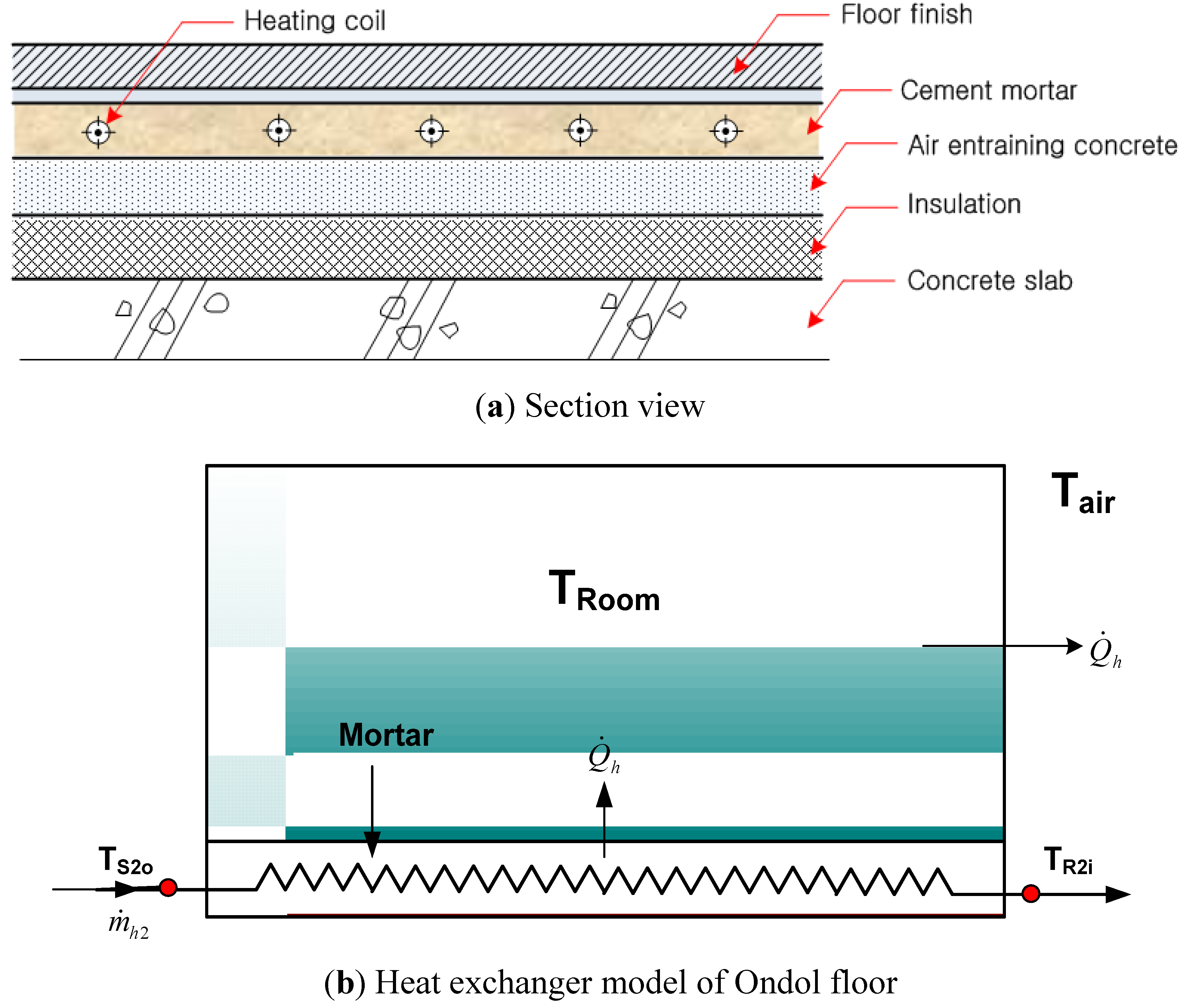
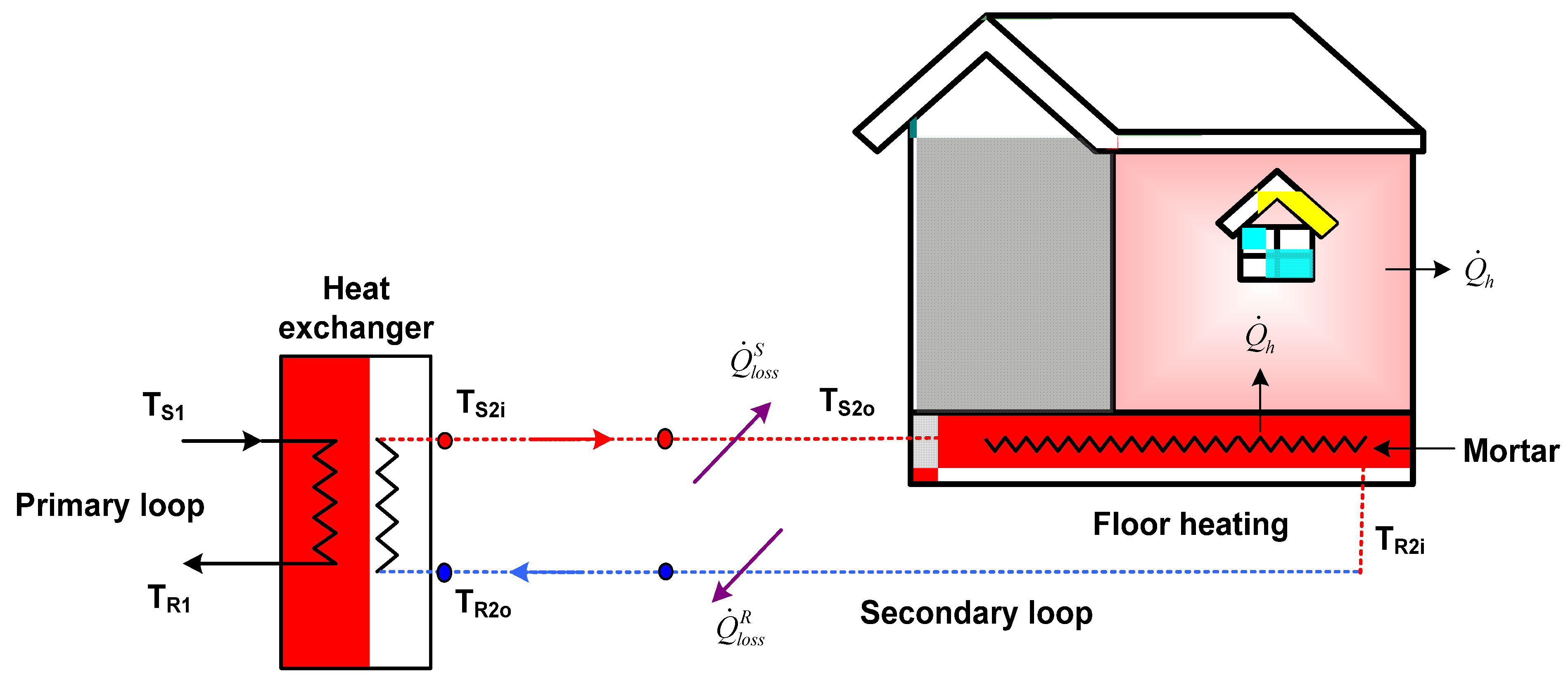
4.1. Heat Exchange Model of Traditional Korean Floor Heating

Figure 11 shows traditional Korean Ondol floor heating system. Figure 11(a) is a sectional view of Ondol floor heating system. The Ondol system is different from radiant systems. Ondol uses water to heat floors. The water line is installed in the floor mortar. The Ondol heating system is modeled as a heat exchanger. The heat exchanger model is shown in Figure 11(b).

The supply water temperature entering the heat supply system is denoted as T_S2o, the mass flow rate as ${\dot{m}}_{h2}$, and the heat capacity of the supply water as C_p. The heat energy of the supply water is transferred indoor through the mortar in the Ondol floor, and then transferred to outdoor through the window, wall, and ceiling. By modeling the Ondol floor as a heat exchanger, T_R2o is the inlet temperature of the Ondol heat exchanger, T_R2i is the outlet temperature of the Ondol heat exchanger, A_Room is the total heating area of the Ondol hot water line, U_Room is the equivalent heat transfer coefficient between the Ondol pipeline and room air. Based on the heat exchanger theorem, the outlet temperature of the Ondol heat exchanger T_R2i is determined from T_Room, T_S2o and (U_RoomA_Room)/( ${\dot{m}}_h{C}_p$) as shown in the following Equation.

$$T_{R2i}=T_{Room}+\left(T_{S2o}-T_{Room}\right)e^{-\frac{(U_{Room}{A}_{Room})}{({\dot{m}}_h{C}_p)}}=T_{Room}+\left(T_{S2o}-T_{Room}\right)e^{-\alpha }$$

(6)

where $(U_{Room}{A}_{Room})/({\dot{m}}_h{C}_p)$ is expressed as α.

Figure 11. Traditional Korean Ondol floor heating system.

Figure 11. Traditional Korean Ondol floor heating system.

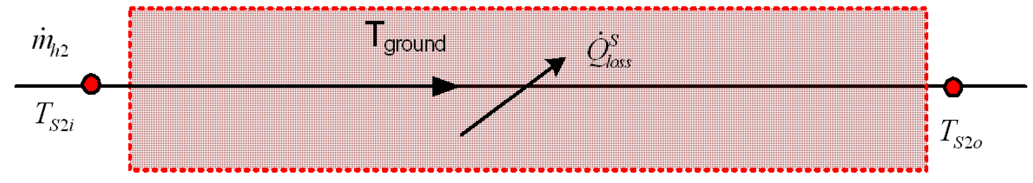
4.2. Heat Loss Rate at the Supply Water Line

Figure 12 is a schematic of the heat loss model of the supply water line. The supply water line connecting the machinery room to the apartment building can be assumed as a heat exchanger. Then, the total heating area of the supply water line is A_s, and U_s is equivalent heat coefficient between the supply water and the wall surrounding the water line. The supply water line is not exposed to air, but is buried underground. Defining T_g as the equivalent temperature of the underground near the supply water line, the supply water line outlet temperature becomes the Ondol inlet temperature T_S2o and based on the heat exchanger theorem:

$$T_{S2o}=T_g+\left(T_{S2i}-T_g\right)e^{-\frac{(U_S{A}_S)}{({\dot{m}}_{h2}{C}_p)}}$$

(7)

where $(U_S{A}_S)/({\dot{m}}_{h2}{C}_p)$ is expressed as ${\beta }_S$.

Meanwhile, the heat loss rate at the supply water line can be expressed as follows using Equation (7):

$$\begin{array}{c}{\dot{Q}}_{loss}^S=C_p{\dot{m}}_{h2}\left[T_{S2i}-T_{S2o}\right]\\ =C_p{\dot{m}}_{h2}\left[T_{S2i}-T_g-\left(T_{S2i}-T_g\right)e^{-{\beta }_S}\right]\end{array}$$

(8)

Substituting Equation (7) into Equation (6) yields,

$$T_{R2i}=T_{Room}+\left[T_g+\left(T_{S2i}-T_g\right)e^{-{\beta }_S}-T_{Room}\right]e^{-\alpha }$$

(9)

Figure 12. Heat loss model of supply water line.

Figure 12. Heat loss model of supply water line.

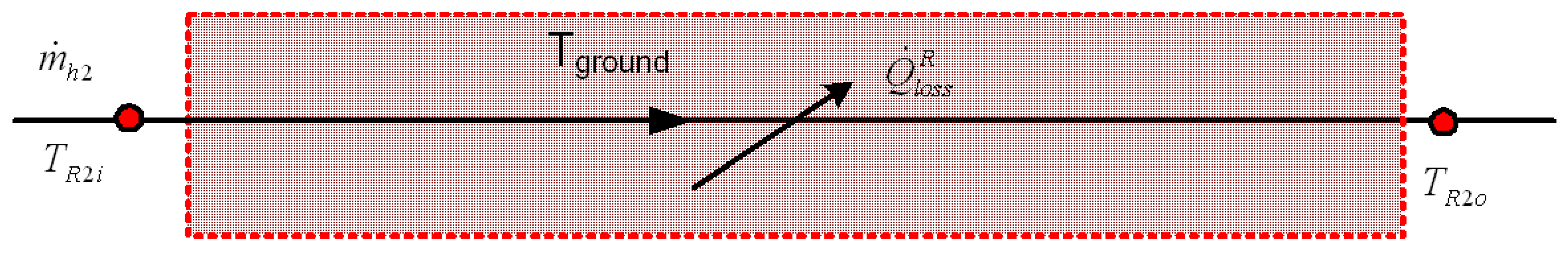
4.3. Heat Loss Rate at the Return Water Line

Figure 13 is a schematic of the heat loss model of return water line. Assuming the return water line as a heat exchanger yields:

$$T_{R2o}=T_g+\left(T_{R2i}-T_g\right)e^{-\frac{U_R{A}_R}{{\dot{m}}_{h2}{C}_p}}$$

(10)

where, T_R2i is the return water line inlet temperature, T_R2o is the return water line heat exchanger outlet temperature, A_R is the total heating area of return water line, and U_R is the equivalent heating coefficient between the return water line and ground. Based on Equation (10), the heat loss rate at the return water line can be expressed by the following Equation:

$$\begin{array}{c}{\dot{Q}}_{loss}^R=C_p{\dot{m}}_{h2}\left(T_{R2i}-T_{R2o}\right)\\ =C_p{\dot{m}}_{h2}\left[T_{R2i}-T_g-\left(T_{R2i}-T_g\right)e^{-{\beta }_R}\right]\end{array}$$

(11)

Figure 13. Heat loss model of return water line.

Figure 13. Heat loss model of return water line.

Meanwhile, assuming that size, length and heating conditions between the supply water line and the return water line are the same, ${\beta }_S={\beta }_R=\beta$ from Equation (10) and Equation (13). In this condition, when Equation (11) and Equation (14) are summed, the total heat loss rate is:

$$\begin{array}{c}{\dot{Q}}_{loss}={\dot{Q}}_{loss}^S+{\dot{Q}}_{loss}^R=C_p{\dot{m}}_h\left(1-e^{-{\beta }_R}\right)\left(T_{S2i}+T_{R2i}-2T_g\right)\\ =C_p{\dot{m}}_h\left(1-e^{-\beta }\right)\left[\left(T_{S2i}-T_g\right)\left(1+e^{-\beta }{e}^{-\alpha }\right)+\left(T_{Room}-T_g\right)\left(1-e^{-\alpha }\right)\right]\end{array}$$

(12)

The heat load of the apartment building is:

$$\begin{array}{c}{\dot{Q}}_h=\dot{m}{C}_p\left(T_{S2o}-T_{R2i}\right)={\dot{m}}_h{C}_p\left[T_{air}+\left(T_{S2i}-T_{air}\right)e^{-{\beta }_S}-T_{Room}-\left(T_{air}+\left(T_{S2i}-T_{air}\right)e^{-{\beta }_S}-T_{Room}\right)e^{-\alpha }\right]\\ ={\dot{m}}_h{C}_p\left[\left(1-e^{-\alpha }\right)\left(T_{air}-T_{Room}\right)+\left(T_{S2i}-T_{air}\right)e^{-{\beta }_S}\left(1-e^{-\alpha }\right)\right]\\ ={\dot{m}}_h{C}_p\left[1-e^{-\alpha }\right]\left[\left(T_{air}-T_{Room}\right)\left(T_{S2i}-T_{air}\right)e^{-{\beta }_S}\right]\end{array}$$

(13)

Organizing Equation (13) with respect to T_S2i yields:

$$T_{S2i}=\left[\frac{{\dot{Q}}_h\left(T_{Room},T_{air}\right)}{{\dot{m}}_{h2}{C}_p\left(1-e^{-\alpha }\right)}+T_{Room}-T_{air}\right]/e^{-{\beta }_S}+T_{air}$$

(14)

If ${\dot{Q}}_h$, U_SA_S, U_RA_R, U_RoomA_Room are known, T_S2i and ${\dot{m}}_h$, which supply ${\dot{Q}}_h$ while minimizing ${\dot{Q}}_{loss}$, can be found from Equations (12) and (14) by computational simulation. Then, the optimal heat supply control algorithm can be utilized.

5. Results and Discussion

Apartments with room temperature of 22 °C were obtained by determining T_Room, as shown in Figure 6, by solving the annual energy consumption with the thermal resistance-capacitance method [21,22] as T_Room is varied. Figure 14 shows the comparison of heat load determined by the thermal resistance-capacitance method and the heat consumption of the target apartment. The two results agree well from March to November, but the heat consumption of the target apartment is slightly higher from the 1st of January to the 28th of February. The result suggests that the room temperature is higher than 22 °C during January and February.

The optimal supply water temperature is shown in Figure 15. Figure 15 is a comparison of the original and the optimal supply water temperature during a day. With the variable supply water temperature system, T_S2i is changed simultaneously with what, resulting in lower supply water temperature. Thus, the heat loss of in the pipeline is reduced.

Figure 16 shows the return water temperature to the heat exchanger. The return water temperature changes according to the outdoor temperature in the optimal heat supply system. T_R2o is lower during Spring, Summer, and Autumn compared to that in the original system.

Figure 17 is the variation of ${\dot{m}}_h$ in the optimal heat supply system. ${\dot{m}}_h$ varies greatly with the outdoor temperature. Thus, the optimal heat supply system increases ${\dot{m}}_h$ and lowers T_S2i. Also, the variations of ${\dot{m}}_h$ of T_S2i according to outdoor temperature were obtained.

Figure 18 is a comparison of the heat loss for the original and the optimal heat supply system. In this study, the optimal heat supply control system was able to meet the heat demand on the consumer side at the lowest supply water temperature and return water temperature, which resulted in 10.4% less energy loss than the case of the original heat supply system.

Figure 14. Annual variation of heating load of the model group energy apartment building.

Figure 14. Annual variation of heating load of the model group energy apartment building.

Figure 15. Comparison of experimental and optimized simulation data of supply water temperatures at group energy apartment building during a day for a year.

Figure 15. Comparison of experimental and optimized simulation data of supply water temperatures at group energy apartment building during a day for a year.

Figure 16. Comparison of experimental and optimized simulation data of temperatures of heat exchanger of group energy apartment building during a day for a year.

Figure 16. Comparison of experimental and optimized simulation data of temperatures of heat exchanger of group energy apartment building during a day for a year.

Figure 17. Comparison of mass flow rate of group energy apartment building with original heating system and that with the optimal heating system for a year.

Figure 17. Comparison of mass flow rate of group energy apartment building with original heating system and that with the optimal heating system for a year.

Figure 18. Comparison of heat loss for a year for original and optimal heat supply system.

Figure 18. Comparison of heat loss for a year for original and optimal heat supply system.

6. Conclusions

In this study, energy loss according to supplied heat was analyzed by developing an optimal heat supply algorithm for group energy apartment buildings. The optimal heat supply control algorithm based on outdoor temperature and heat load curve calculation was also studied.

The results can be summarized as follows.

(1)

This study was based on the apartment building heat consumption data collected in year 2008. Thus, if an accurate database on heat supply and consumption pattern can be obtained, the developed system can accurately predict heat load variations according to outdoor temperature.

(2)

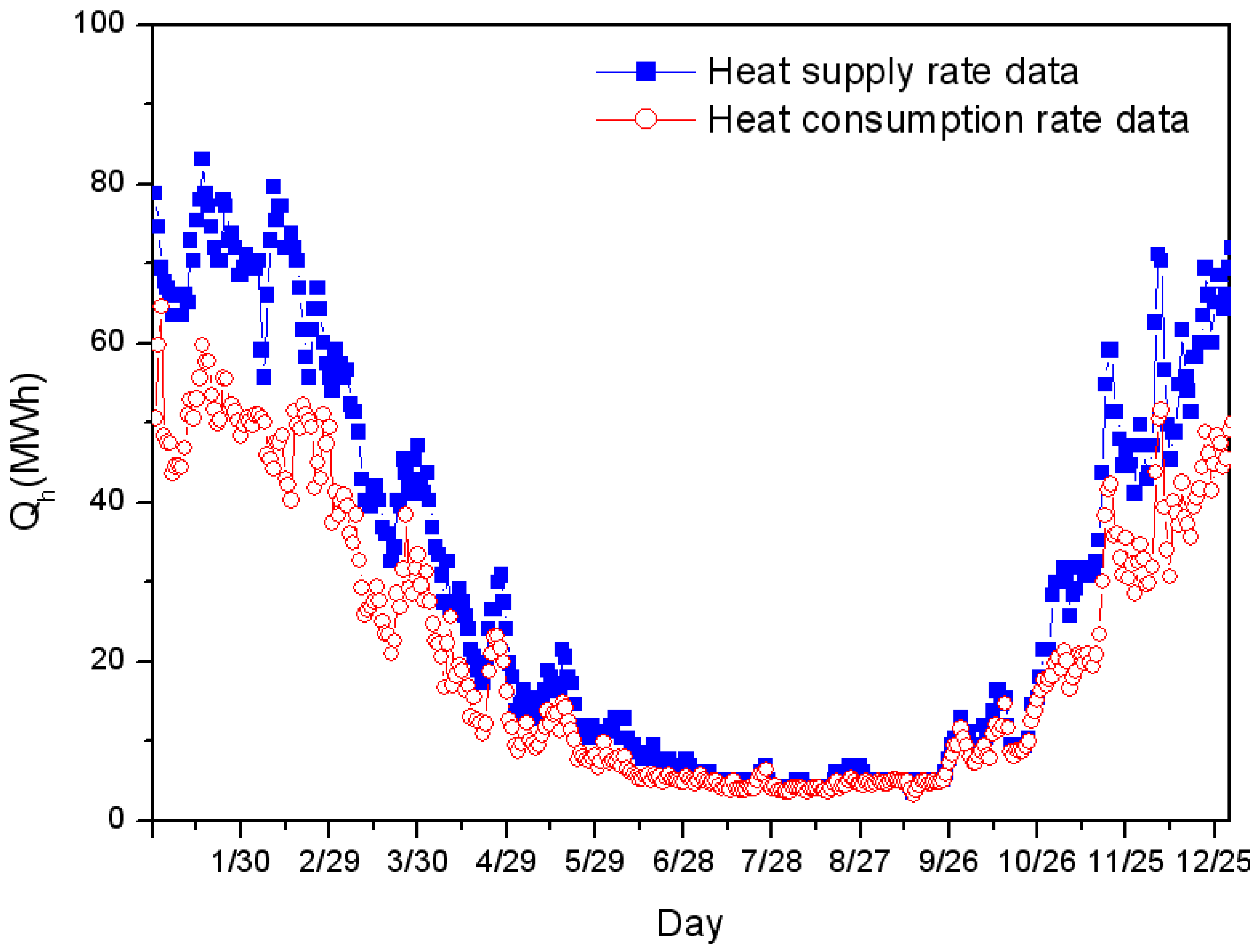
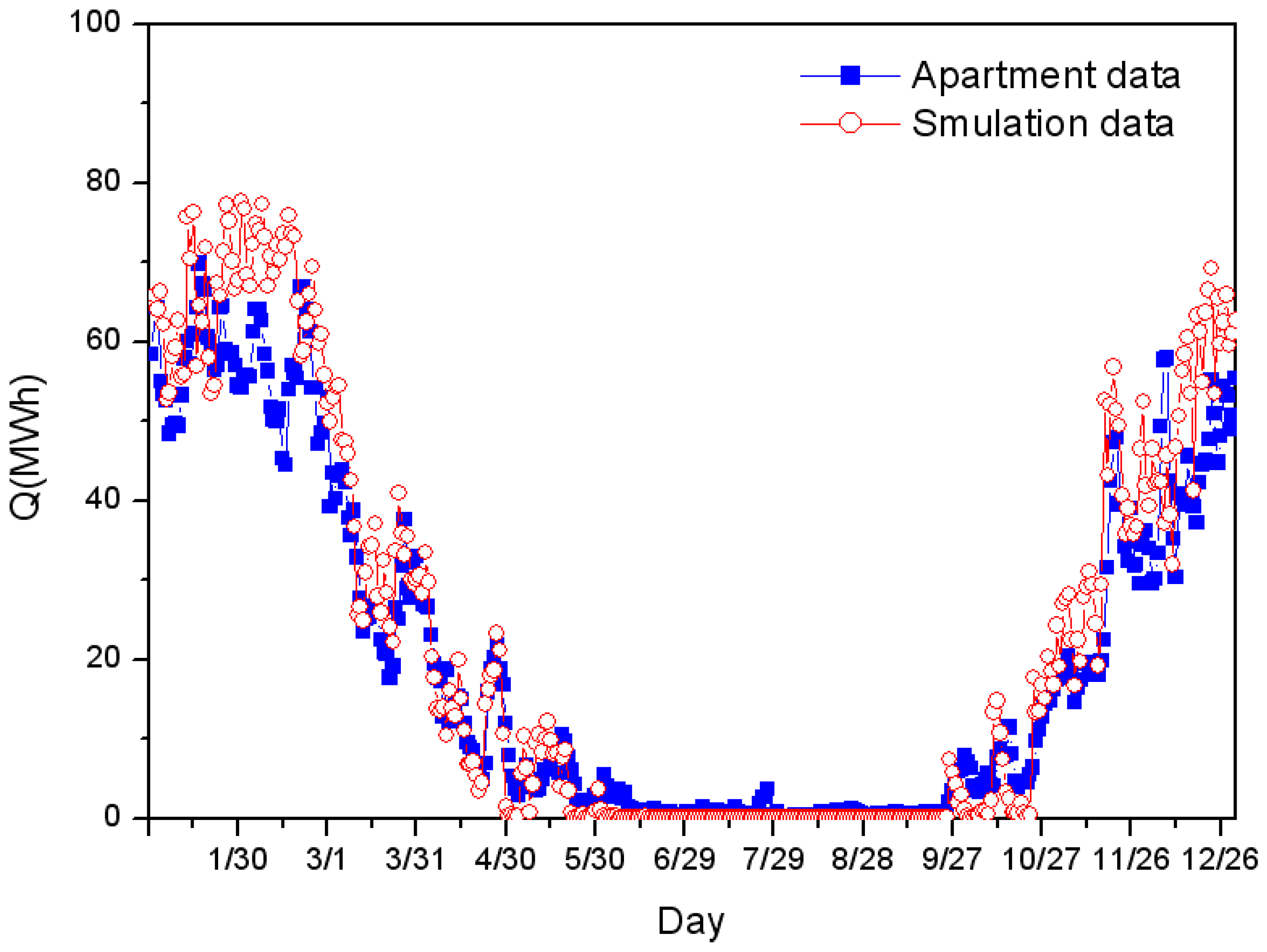
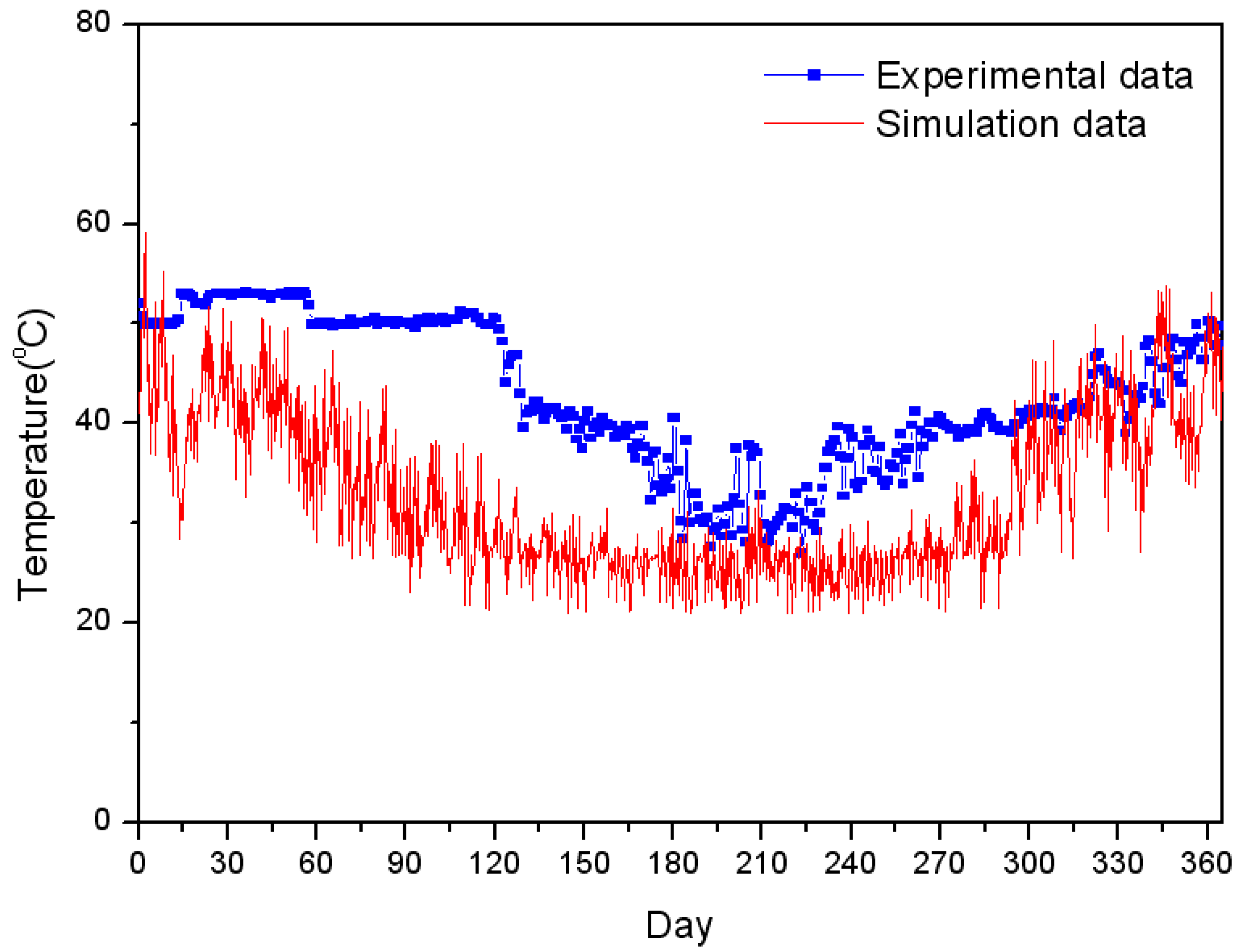
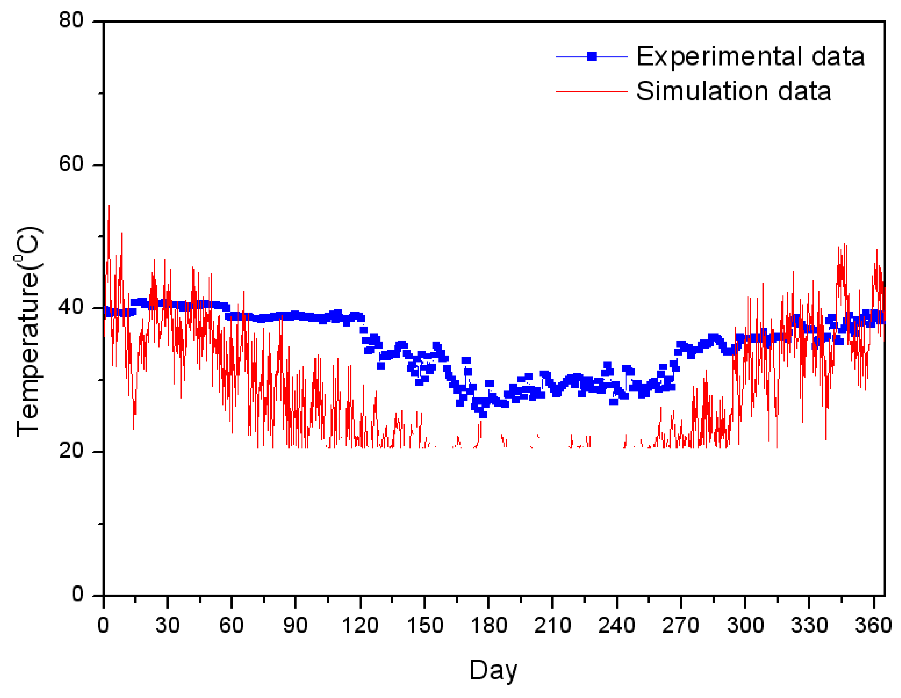
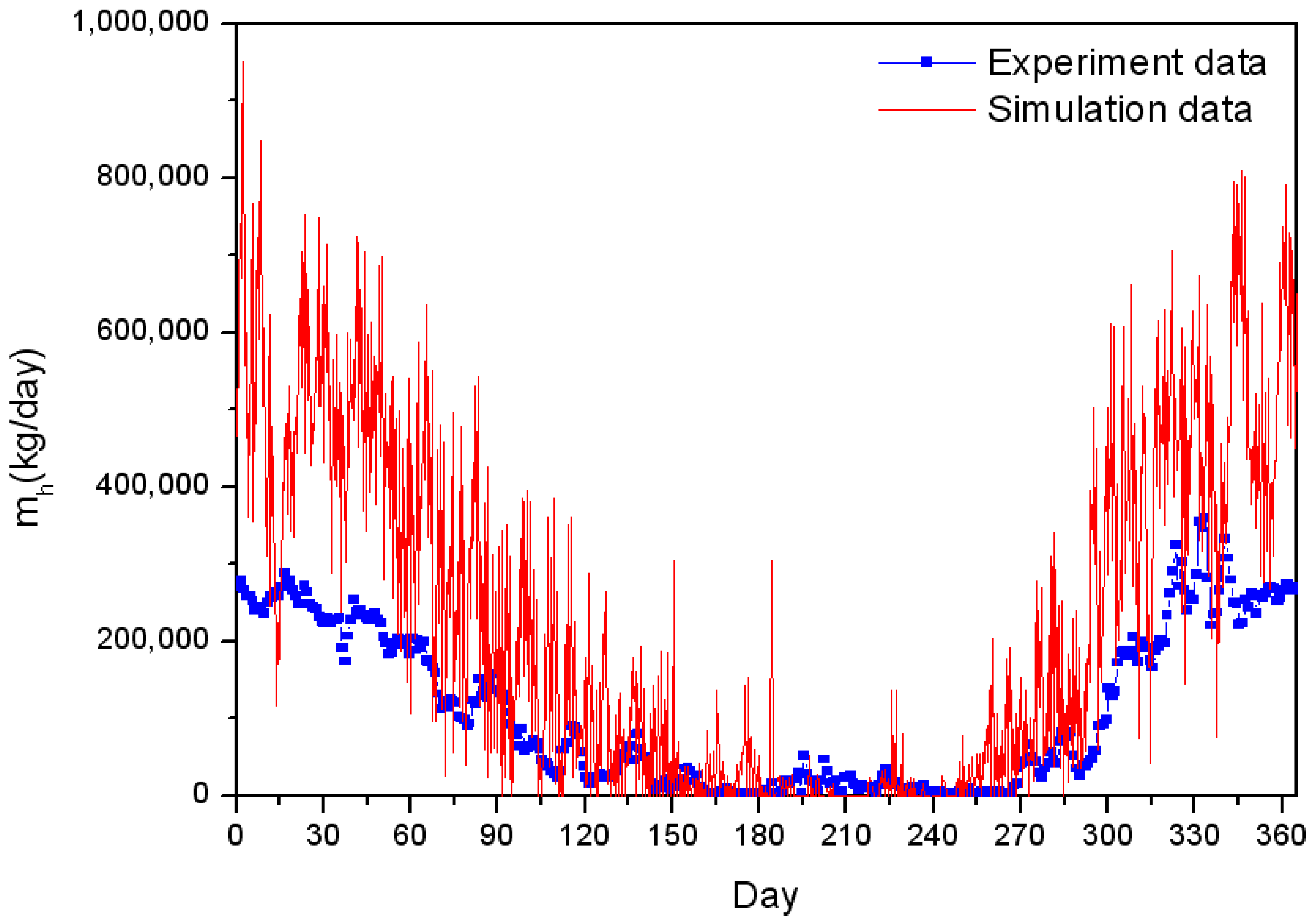
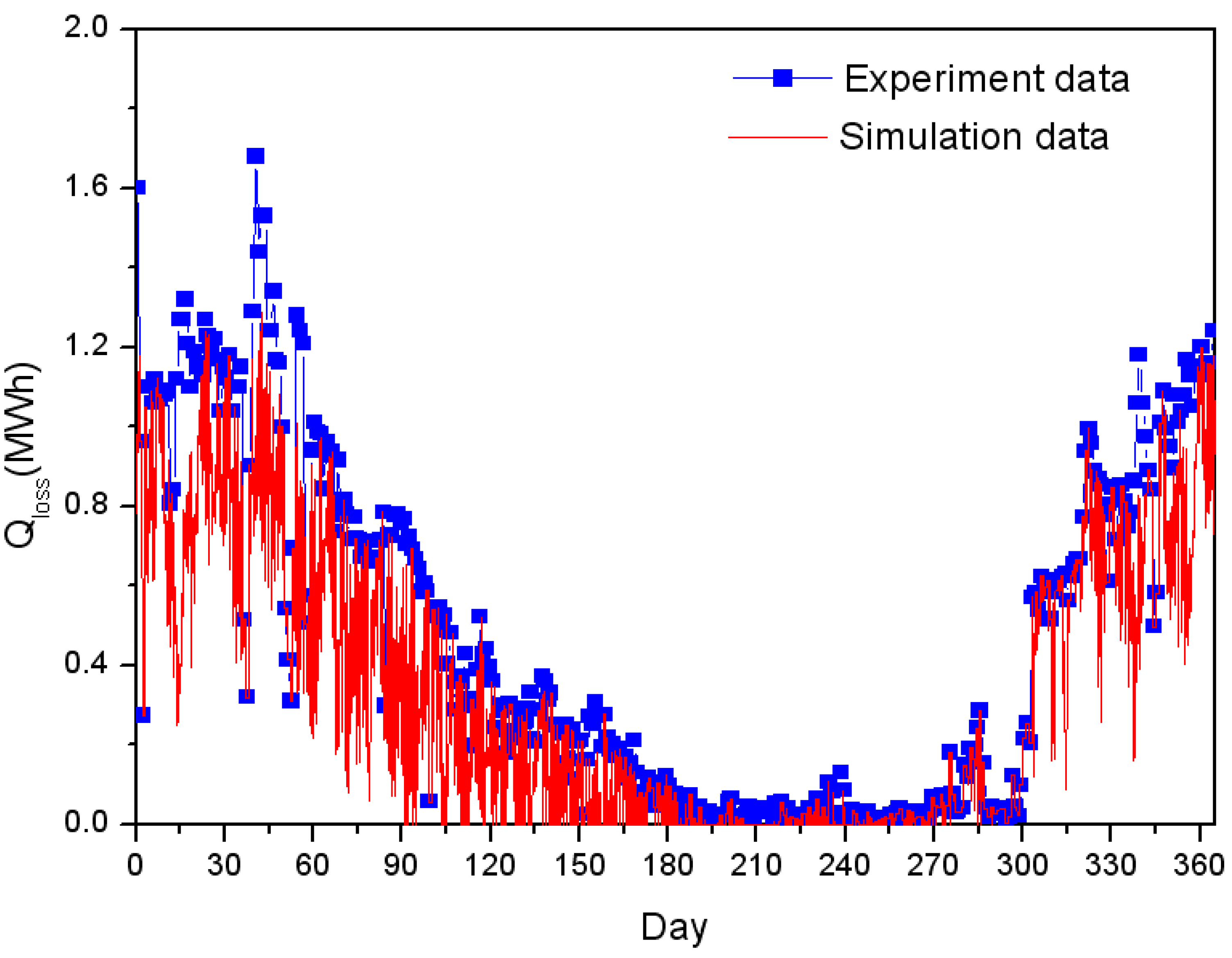
Heat load was predicted for group energy apartment buildings. The predictions were compared with experimental data for validation. The results of the heat load prediction method for group energy apartment buildings agreed well with experimental data.

(3)

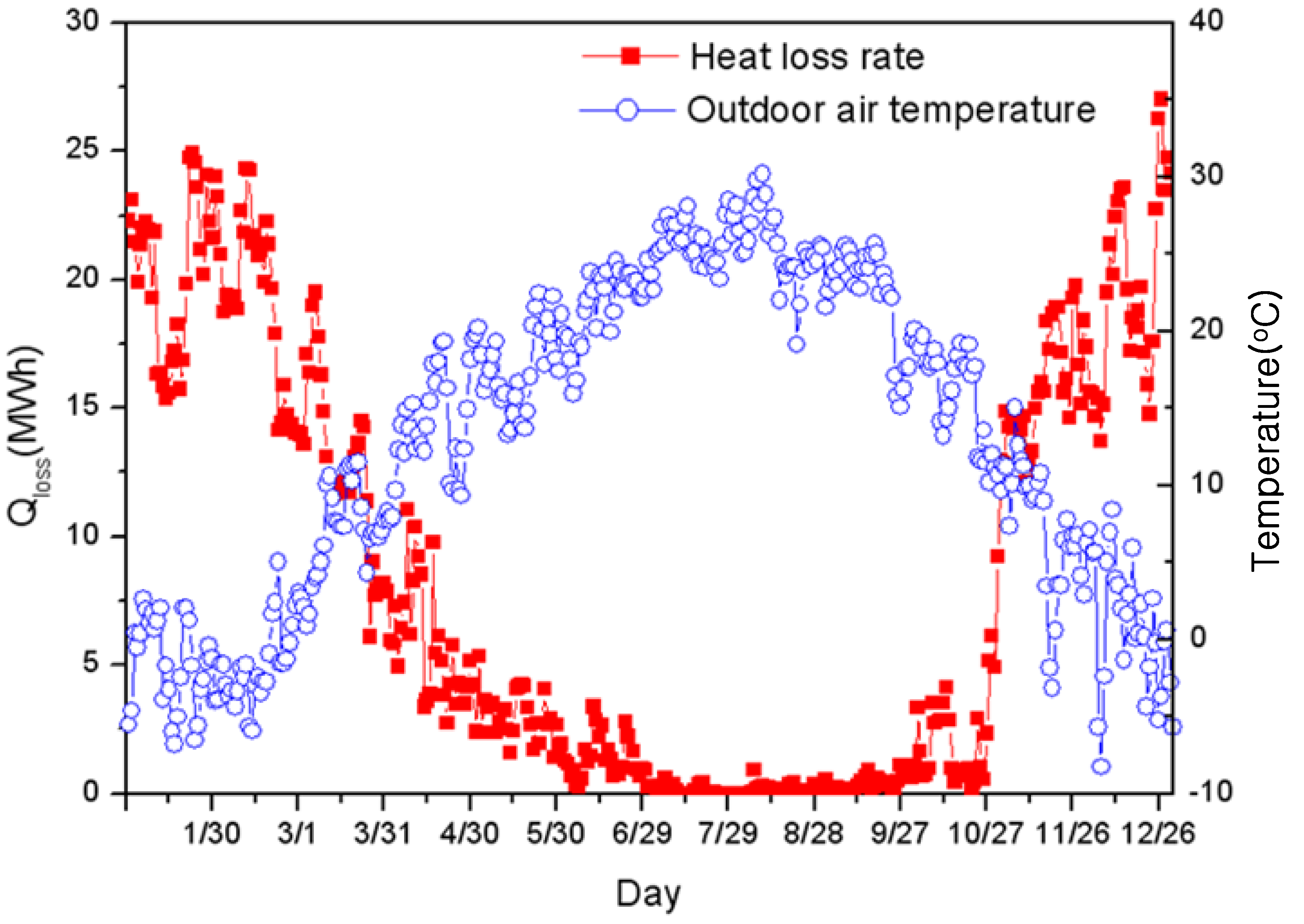
In this study, energy loss was decreased by 10.4% compared to the supply heat by applying the lowest supply water temperature and return water temperature in the optimal heat supply control system.

(4)

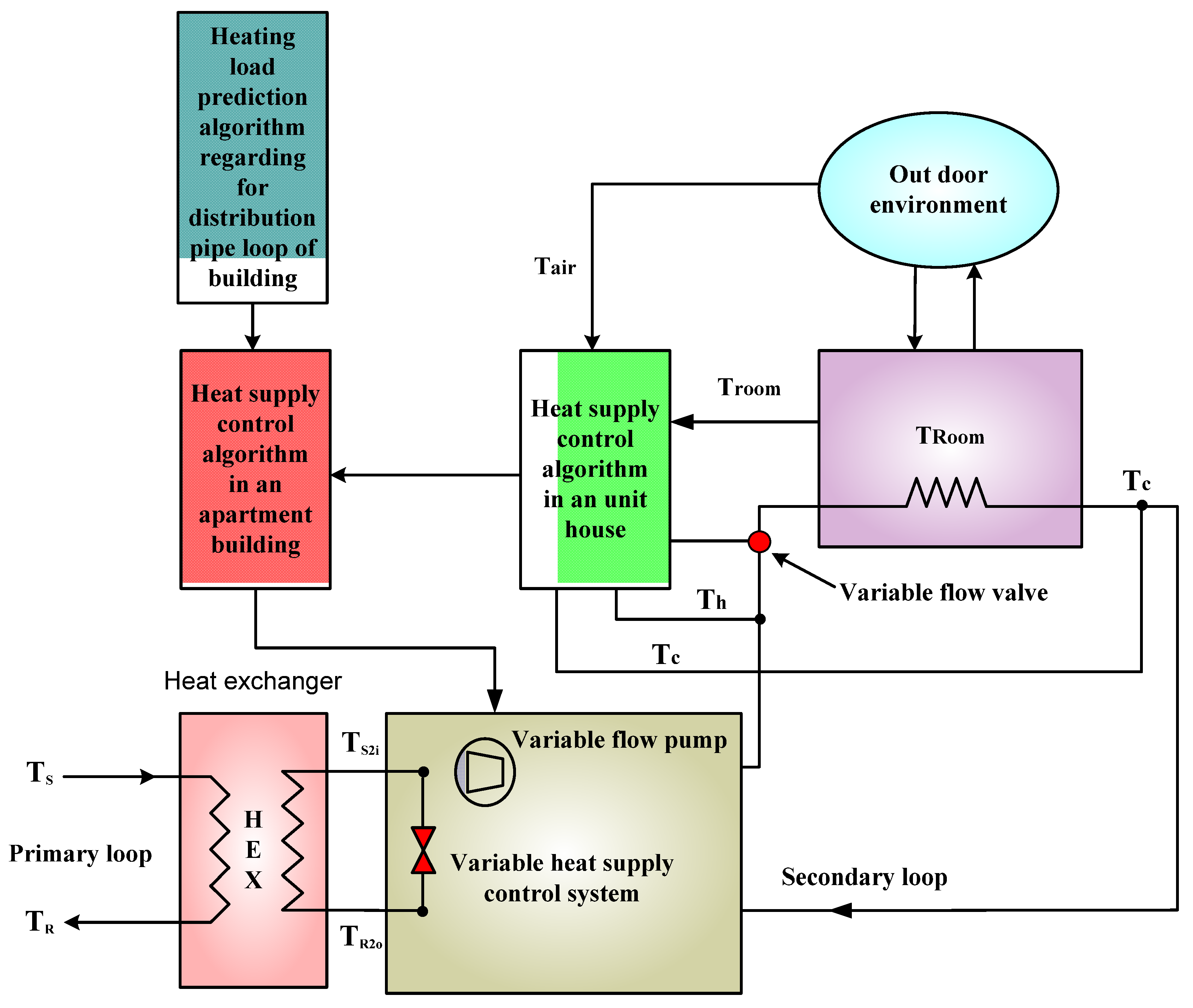
Heat supply control can be achieved by variable supply mass flow rate control and variation supply water temperature control. To meet consumer heat capacity needs, mass flow rate is varied according to supply water temperature. Low mass flow rate is applied for high supply water temperature, while mass flow rate is increased when the supply water temperature is low.

(5)

Primary return water temperature without affecting the indoor temperature. Thus a better utilization of the heat generated from heat generation facility is achievable. The optimal primary side supply water temperature is found when the return water temperature reaches its minimum under the heat control algorithm.

(6)

Analysis results of this study can be used to evaluate heat consumption patterns according to outdoor temperature. The analysis results suggest that further research in this area could lead to substantial energy savings in apartment buildings.

References

1. Bøhm, B.; Danig, P.O. Monitoring the energy consumption in a district heated apartment building in Copenhagen, with specific interest in the thermodynamic performance. Energy Build. 2004, 36, 229–236. [Google Scholar]
2. Stevanovic, V.D.; Prica, S.; Maslovaric, B.; Zivkovic, B.; Nikodijevic, S. Efficient numerical method for district heating system hydraulics. Energy Convers. Manag. 2007, 48, 1536–1543. [Google Scholar] [CrossRef]
3. Wu, Y.G.; Rosen, M.A. Assessing and optimizing the economic and environmental impacts of cogeneration/district energy systems using an energy equilibrium model. Appl. Energy 1999, 62, 141–154. [Google Scholar] [CrossRef]
4. Dotzauer, E. Experiences in mid-term planning of district heating systems. Energy 2003, 28, 1545–1555. [Google Scholar] [CrossRef]
5. Dotzauer, E. Simple model for prediction of loads in district-heating systems. Appl. Energy 2002, 73, 277–284. [Google Scholar] [CrossRef]
6. Heller, A.J. Heat-load modelling for large systems. Appl. Energy 2002, 72, 371–387. [Google Scholar] [CrossRef]
7. Knutsson, D.; Sahlin, J.; Werner, S.; Ekvall, T.; Ahlgren, E.O. HEATSPOT—A simulation tool for national district heating analyses. Energy 2006, 31, 278–293. [Google Scholar] [CrossRef]
8. Shimoda, Y.; Nagota, T.; Isayama, N.; Mizuno, M. Verification of energy efficiency of district heating and cooling system by simulation considering design and operation parameters. Build. Environ. 2006, 43, 569–577. [Google Scholar] [CrossRef]
9. Fu, L.; Yi, J.; Yuan, W.; Qin, X. Influence of supply and return water temperatures on the energy consumption of a district cooling system. Appl. Therm. Eng. 2001, 21, 511–521. [Google Scholar] [CrossRef]
10. Larsen, H.V.; Palsson, H.; Bøhm, B.; Wigbels, M. A comparison of aggregated models for simulation and operational optimisation of district heating networks. Energy Convers. Manag. 2004, 45, 1119–1139. [Google Scholar] [CrossRef]
11. Salsbury, T.; Diamond, R. Performance validation and energy analysis of HVAC system using simulation. Energy Build. 2000, 21, 5–17. [Google Scholar] [CrossRef]
12. Bojic, M.; Trifunovic, N.; Gustafsson, S.I. Mixed 0–1 sequential linear programming optimization of heat distribution in a district-heating system. Energy Build. 2000, 32, 309–317. [Google Scholar] [CrossRef]
13. Nielsen, H.; Madsen, H. Modelling the heat consumption in district heating systems using a grey-box approach. Energy Build. 2000, 38, 63–71. [Google Scholar] [CrossRef]
14. Holmgren, K.; Gebremedhin, A. Modelling a district heating system: Introduction of waste incineration, policy instruments and co-operation with an industry. Energy Policy 2004, 32, 1807–1817. [Google Scholar] [CrossRef]
15. Henning, D.; Amiri, S.; Holmgren, K. Modelling and optimisation of electricity, steam and district heating production for a local Swedish utility. Eur. J. Oper. Res. 2006, 175, 1224–1247. [Google Scholar] [CrossRef]
16. Gabrielaitiene, I.; Bøhm, B.; Sunden, B. Modelling temperature dynamics of a district heating system in Naestved, Denmark—A case study. Energy Convers. Manag. 2007, 48, 78–86. [Google Scholar] [CrossRef]
17. Lianzhong, L.; Zaheeruddin, M. A control strategy for energy optimal operation of a direct district heating system. Int. J. Energy Res. 2004, 28, 597–612. [Google Scholar] [CrossRef]
18. Langendries, R. Low return temperature (LRT) in district heating. Energy Build. 1998, 12, 191–200. [Google Scholar] [CrossRef]
19. Kim, M.H. Low Thermal Quantity and Pattern of Special Facilities Connected by a District Heat. M.S. Thesis, Hanyang University, Seoul, Korea, February 2007. [Google Scholar]
20. Kim, S.K.; Lee, D.H.; Hong, H.K. An energy saving technique using Ondol heating schedule control of housing units in Korea. Indoor Built Environ. 2009, 19, 88–93. [Google Scholar] [CrossRef]
21. Lee, C.S.; Choi, Y.D. Analysis of energy consumption of office building by thermal resistance-capacitance method. Korea J. Air-Cond. Ref. Eng. 1997, 9, 1–13. [Google Scholar]
22. Yoon, J.H.; Hong, J.K.; Lee, N.H.; Choi, Y.D. Simulation of thermal performance of model hot water panel house in consideration of radiant heat transfer. Korea J. Air-Cond. Ref. Eng. 1993, 5, 295–305. [Google Scholar]