1. Introduction
Wind power has experienced a rapid global growth since the late 1990s. In the year 1997, there was only 7480 MW of installed capacity worldwide. Initially, this capacity was increased by about 2000 MW per year. However this annual growth rate has been increased until reaching a rate of 42 GW that were added in 2011 after 37.6 GW added in 2010, 38.3 GW added in 2009 and 27 GW added in 2008. In this sense the worldwide wind power installed capacity reaches 239 GW in 2011, and an annual growth rate of 60 GW in 2012 and 100 GW in 2013 is expected [
1].
The high growth rate of wind power capacity is explained by the cost reduction as well as by new public government subsides in many countries linked to efforts to increase the use of renewable power production and reduce CO emissions.
All wind turbines installed by the end of 2010 worldwide are generating 430 TWh per annum, equaling more than 2.5% of the global electricity consumption, and it is expected that this percentage will increase in the following years. However, wind power production is highly dependent on the wind resources at the local site.
In 2010, the Chinese wind market became a class of its own, representing more than half of the world market for new wind turbines adding 18.9 GW, which equals a market share of 50.3%. A sharp decrease in new capacity happened in the USA, whose share in new wind turbines fell down to 14.9% (5.6 GW), after 25.9% (9.9 GW) in the year 2009. Nine further countries could be seen as major markets, with turbine sales in a range between 0.5 and 1.5 GW: Germany, Spain, India, United Kingdom, France, Italy, Canada, Sweden and the Eastern European newcomer Romania. Again twelve markets for new turbines had a medium size between 100 and 500 MW: Turkey, Poland, Portugal, Belgium, Brazil, Denmark, Japan, Bulgaria, Greece, Egypt, Ireland, and Mexico. By end of 2010, 20 countries had installations of more than 1000 MW, compared with 17 countries by end of 2009 and 11 countries by end of 2005. Worldwide, 39 countries had wind farms with a capacity of 100 MW or more installed, compared with 35 countries one year ago, and 24 countries five years ago. The top five countries (USA, China, Germany, Spain and India) represented 74.2% of the worldwide wind capacity, significantly more than 72.9% in the year 2009. The USA and China together represented 43.2% of the global wind capacity (up from 38.4% in 2009). Due to the strong performance of the Chinese market, a certain concentration process of the world market on China can be observed, with China alone representing more than half of the market for new wind turbines. The newcomer on the list of countries using wind power commercially is a Mediterranean country, Cyprus, which for the first time installed a larger grid-connected wind farm, with 82 MW.
In some countries and regions wind has become one of the largest electricity sources. Again in terms of wind share, Denmark is the world leader. The countries with the highest wind shares are: Denmark (21%), Portugal (18%), Spain (16%) and Germany (9%). In China, wind contributed 1.2% to the overall electricity supply, while in the USA the wind share has reached about 2%.
Based on the experience and growth rates of the past years, World Wind Energy Association (WWEA) expects that wind energy will continue its dynamic development also in the coming years. Although the short term impacts of the current finance crisis makes short-term predictions rather difficult, it can be expected that in the mid-term wind energy will rather attract more investors due to its low risk character and the need for clean and reliable energy sources. More and more governments understand the manifold benefits of wind energy and are setting up favorable policies, including those that are stimulation decentralized investment by independent power producers, small and medium sized enterprises and community based projects, all of which will be main drivers for a more sustainable energy system also in the future.
Carefully calculating and taking into account some insecurity factors, in 2015, a global capacity of 600 GW is possible. By the end of year 2020, at least 1500 GW can be expected to be installed globally and then wind energy will be able to contribute in the year 2020 at least 12% of global electricity consumption. However the large wind power penetration faces a variety of technical problems and challenges such as frequency and voltage regulation, power quality issues, electromagnetic interference,
etc. [
2,
3,
4,
5], which should be addressed in order to further increase the wind power penetration.
The Doubly Fed Induction Generator (DFIG), with vector control applied, is widely used in variable speed wind turbine control system owing to their ability to maximize wind power extraction and to their capability to fulfill the basic technical requirements set by the system operators and contribute to power system security [
6,
7,
8]. In these DFIG wind turbines the control system should be designed in order to to achieve the following objectives: regulating the DFIG rotor speed for maximum wind power capture, maintaining the DFIG stator output voltage frequency constant and controlling the DFIG reactive power.
One of the main task of the the controller is to carry the turbine rotor speed into the desired optimum speed, in spite of system uncertainties, in order to extract the maximum active power from the wind. This paper investigates a new robust speed control method for variable speed wind turbines, in order to obtain the maximum wind power capture in spite of system uncertainties [
9,
10].
In the last decade, some papers on application of sliding mode control to wind energy systems has been presented.
In the work of [
11] a Sliding Mode Control of Wind Energy Systems with a DFIG is presented. In the proposed design a static Kramer Drive is used as recovery drive. This converter uses a diode rectifier bridge and therefore only allows operation at sub-synchronous speed. In this sense, the rotor power flow only can be sent from the rotor to the DC link. In our proposed design an IGBT based inverter is used and therefore the system can operate at sub-synchronous or at super-synchronous speed.
In the work of [
12] a design method for variable structure system control for a wind energy conversion subsystem is presented. The design is comprised of a turbine directly coupled to a multiple permanent magnet synchronous generator (PMSG), a diode bridge rectifier and a DC/DC converter to adapt voltages. This control scheme uses a full converter. This implies that all the power have to be transmitted to the grid through the converter. Our proposed design uses a DFIG and then the power captured by the wind turbine is converted into electrical power by the DFIG and this power is transmitted to the grid by the stator and the rotor windings. In this scheme, the stator is directly connected to the grid and therefore only the power transmitted from the rotor winding have to be transmitted through the converter.
In the work of [
13] an integral fuzzy sliding mode control method is proposed for control objects with uncertain parameters and force disturbances. The proposed method is applied to generator speed tracking control of a large-scale variable speed wind power system in Section III. However this design uses a linearized model of the wind turbine system. Moreover, this design do not take into account the generator dynamics. Our proposed design do not use a linearized model of the wind turbine system and takes into account the generator dynamics.
In the work of [
14] the energy reliability optimization of wind energy conversion systems’ operation using a sliding mode control is presented. The proposed approach aims at designing a trade-off between maximizing the power harvested from the wind by a variable-speed doubly-fed-induction-generator-based wind power system and minimizing its mechanical stress. The proposed design uses a sliding surface that depends on the optimal shaft speed and the optimal electromagnetic torque that depends on the wind speed. Therefore the sliding surface changes with the wind speed too and then the system lost the sliding mode and hence the maximum power point tracking when the wind speed changes. In our proposed design the sliding surface do not depend on the wind and therefore the system do not lose the sliding mode when the wind speed changes.
Basically, the proposed robust design uses the sliding mode control algorithm to regulate both the rotor-side converter (RSC) and the grid-side converter (GSC). In the design a vector oriented control theory is used in order to decouple the torque and the flux of the induction machine. This control scheme leads to obtain the maximum power extraction from the different wind speeds that appear along time.
Finally, some tests of the proposed method based on a two-bladed horizontal axis wind turbine are conducted using the Matlab/Simulink software. In this test, several operating conditions are simulated and satisfactory results are obtained.
2. Problem Statement
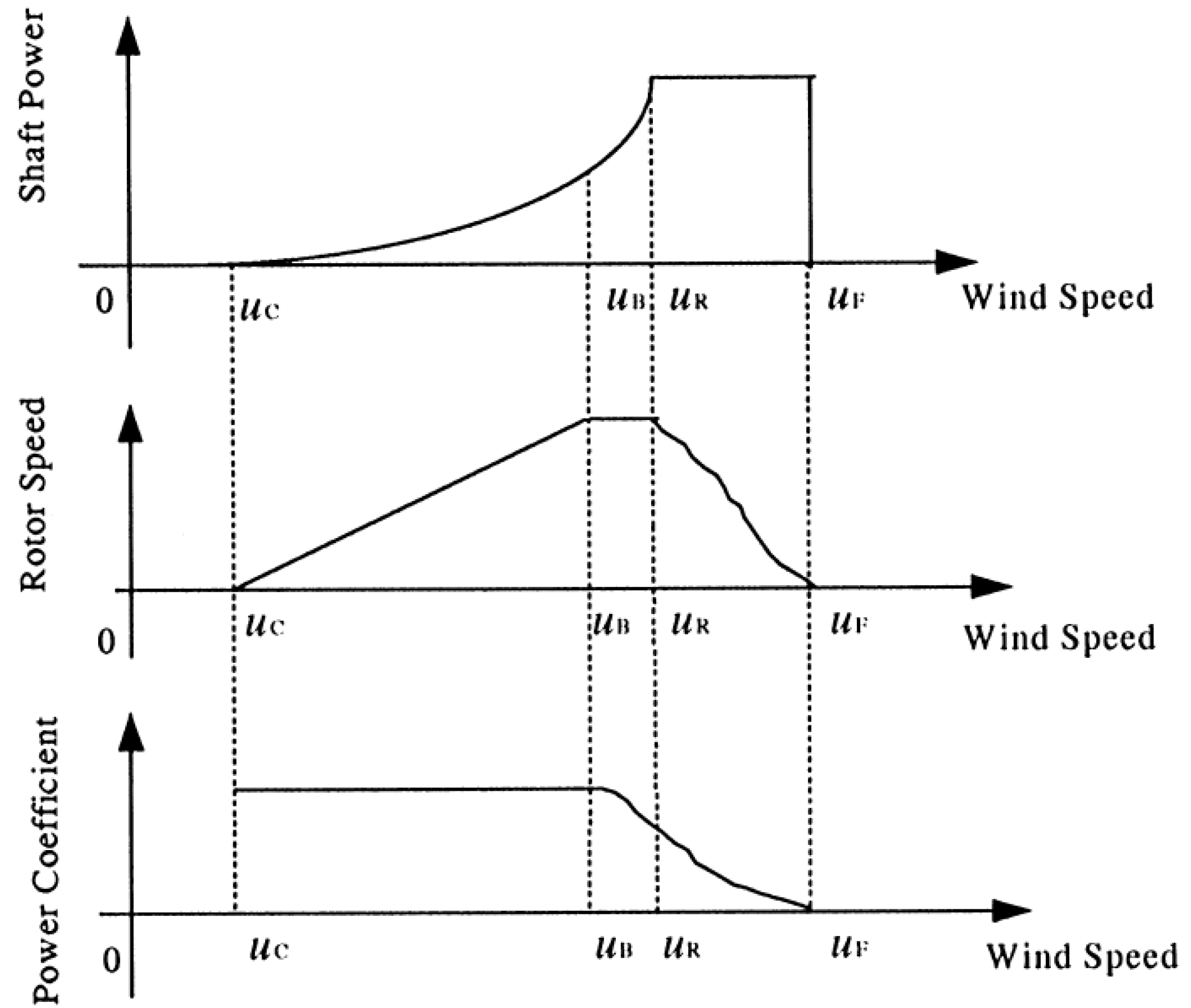
There are three fundamental modes of operation in order to extract effectively wind power while at the same time maintaining safe operation [
15]. In these modes illustrated in
Figure 1 the wind turbine should be driven according to:
Mode 1 Operation at variable speed/optimum tip-speed ratio:
Mode 2 Operation at constant speed/variable tip-speed ratio:
Mode 3 Operating at variable speed/constant power:
where
u is the wind speed,
is the cut-in wind speed,
denotes the wind speed at which the maximum allowable rotor speed is reached,
is the rated wind speed and
is the furling wind speed at which the turbine needs to be shut down for protection.
Figure 1.
Turbine speed operation modes.
Figure 1.
Turbine speed operation modes.
It is seen that, if high-power efficiency is to be achieved at lower wind speeds, the rotor speed of the wind turbine must be adjusted continuously against wind speed. A common practice in addressing the control problem of wind turbines is to use linearization approach. This method allows the linear system theory to be applied in control design and analysis. However, due to the stochastic operating conditions and the inevitable uncertainties inherent in the system, such a control method comes at the price of poor system performance and low reliability.
In this work we present a method for variable speed control of wind turbines. The objective is to make the rotor speed track the desired speed that is specified according to the three fundamental operating modes as described earlier. This is achieved regulating the rotor currents of the double feed induction generator (DFIG) through the developed nonlinear and robust control algorithms. Such a control scheme leads to more energy output without involving additional mechanical complexity to the system.
3. System Modelling
The power extraction of a wind turbine is a function of three main factors: the wind power available, the power curve of the machine and the ability of the machine to respond to wind fluctuation. The expression for power produced by the wind is given by [
16]:
where
ρ is the air density,
R is the radius of the rotor,
u is the wind speed,
denotes the power coefficient of the wind turbine,
λ is the tip-speed ratio and
β represents the pitch angle.
The tip-speed ratio is defined as:
where
w is the turbine rotor speed. Therefore, if the rotor speed is kept constant, then any change in the wind speed will change the tip-speed ratio, leading to the change of power coefficient
, as well as the generated power output of the wind turbine. However, if the rotor speed is adjusted according to the wind speed variation, then the tip-speed ratio can be maintained at an optimal point, which could yield maximum power output from the system.
For a typical wind power generation system, the following simplified elements are used to illustrate the fundamental work principle. The system primarily consists of an aeroturbine, which converts wind energy into mechanical energy, a gearbox, which serves to increase the speed and decrease the torque, and a generator used to convert the mechanical energy into the electrical energy.
Driving by the input wind torque , the rotor of the wind turbine runs at the speed . The transmission output torque is then fed to the generator, which produces a shaft torque of at generator angular velocity of w. Note that the rotor speed and generator speed are not the same in general, due to the use of the gearbox.
The mechanical equations of the system can be characterized by [
17]:
where
and
are the moment of inertia of the turbine and the generator,
and
are the viscous friction coefficient of the the turbine and the generator,
is the wind generated torque in the turbine,
T is the torque in the transmission shaft before gear box,
is the torque in the transmission shaft after gear box, and
is the the generator torque,
is the angular velocity of the turbine shaft and
w is the angular velocity of the generator rotor.
The relation between the angular velocity of the turbine
w and the angular velocity of the generator
is given by the gear ratio
γ:
Then, using Equations (3–6) it is obtained:
with
From Equations (1,2) it is deduced that the input wind torque is:
where
Now, we are going to consider the system electrical equations. In this work a double feed induction generator (DFIG) is used. This induction machine is fed from both stator and rotor sides. The stator is directly connected to the grid while the rotor is fed through a variable frequency converter (VFC). In order to produce electrical active power at constant voltage and frequency to the utility grid, over a wide operation range (from sub-synchronous to super-synchronous speed), the active power flow between the rotor circuit and the grid must be controlled both in magnitude and in direction. Therefore, the VFC consists of two four-quadrant IGBT PWM converters, the rotor-side converter (RSC) and the grid-side converter (GSC) that are connected back-to-back by a DC-link capacitor [
18].
The DFIG can be regarded as a traditional induction generator with a nonzero rotor voltage. The dynamic equation of a thee-phase DFIG can be written in a synchronously rotating d-q reference frame as [
19].
where
is the rotational speed of the synchronous reference frame,
is the slip frequency and
s is the slip,
is the generator rotor speed and the flux linkages are given by:
where
,
, and
are the stator inductance, rotor inductance and mutual inductances, respectively.
The electrical torque equation of the DFIG is given by:
where
p is the pole numbers.
Neglecting the power loses associated with the stator resistances, the active and reactive stator powers are:
Similarly, the rotor power (also called slip power) can be calculated as:
Then, when the power losses in the converters are neglected, the total real power injected into the grid equals to the sum of the stator power and the rotor power . In the same way, the reactive power exchanged with the grid equals to the sum of stator reactive power and the rotor reactive power .
4. Wind Turbine Control Scheme
The DFIG wind turbine control system should be designed in order to to achieve the following objectives:
Regulating the DFIG rotor speed for maximum wind power capture.
Maintaining the DFIG stator output voltage frequency constant.
Controlling the DFIG reactive power.
In order to achieve these objectives the wind turbine control system are generally composed of two parts: the electrical control on the DFIG and the mechanical control on the wind turbine blade pitch angle [
20]. The control of the DFIG is achieved by controlling the variable frequency converter (VFC), which includes control of the rotor-side converter (RSC) and control of the grid-side converter (GSC). The objective of the RSC is to govern both the stator-side active and reactive powers independently, while the objective of the GSC is to keep the DC-link voltage constant regardless of the magnitude and direction of the rotor power. The GSC control scheme can also be designed to regulate the reactive power or the stator terminal voltage of the DFIG. A typical scheme of a DFIG equipped wind turbine is shown in
Figure 2.
Figure 2.
Scheme of a wind turbine system with a DFIG.
Figure 2.
Scheme of a wind turbine system with a DFIG.
When the wind turbine generator (WTG) operates in the variable-speed mode, in order to extract the maximum active power from the wind, the shaft speed of the WTG must be adjusted to achieve an optimal tip-speed ratio
, which yields the maximum power coefficient
, and therefore the maximum power [
21]. In other words, given a particular wind speed, there is a unique wind turbine speed command to achieve the goal of maximum wind power extraction. The value of the
can be calculated from the maximum of the power coefficient curves versus tip-speed ratio, which depends of the modeling turbine characteristics.
The power coefficient
can be approximated by Equation (
25) based on the modeling turbine characteristics [
22]:
where the coefficients
to
depends on the wind turbine design characteristics, and
is defined as
The value of
can be obtained from Equation (
25) calculating the
λ value that maximizes the power coefficient. Then, based on the wind speed, the corresponding optimal generator speed command for maximum wind power extraction is determined by:
It should be noted that the proposed design is based on the knowledge of the turbine characteristics, and therefore the turbine characteristics should be calculated as accurately as possible in order to obtain a good performance for the system controller.
5. Rotor Side Converter Control
The RSC control scheme should be designed in order to regulate the wind turbine speed for maximum wind power capture. Therefore, a suitably speed controller is essential to track the optimal wind turbine speed reference for maximum wind power extraction. The design of such a speed controller should take into account the wind turbine system dynamics. In the DFIG-based wind generation system, this objective is commonly achieved by the rotor current regulation of the electrical generator using the stator-flux oriented reference frame.
In the stator-flux oriented reference frame, the d-axis is aligned with the stator flux linkage vector
, and then,
and
. This yields the following relationships [
23]:
where
Since the stator is connected to the grid, and the influence of the stator resistance is small, the stator magnetizing current (
) can be considered constant [
18]. Therefore, the electromagnetic torque can be defined as follows:
where
is a torque constant, and is defined as follows:
Then, from Equations (7,36) it is deduced that the wind turbine speed can be controlled by regulating the q-axis rotor current components (), while Equation (31) indicates that the stator reactive power () can be controlled by regulating the d-axis rotor current components, (). Consequently, the reference values of and can be determined directly from w and references.
From Equations (7,36) the following dynamic equation for the system speed is obtained:
where the parameters are defined as:
Now, we are going to consider the previous dynamic Equation (
38) with uncertainties as follows:
where the terms
,
and
represents the uncertainties of the terms
a,
b and
f respectively.
Let us define define the speed tracking error as follows:
where
is the rotor speed command.
Taking the derivative of the previous equation with respect to time yields:
where the following terms have been collected in the signal
,
and the uncertainty terms have been collected in the signal
,
To compensate for the above described uncertainties that are present in the system, a sliding control scheme is proposed. In the sliding control theory, the switching gain must be constructed so as to attain the sliding condition [
24]. In order to meet this condition a suitable choice of the sliding gain should be made to compensate for the uncertainties.
Now, we are going to define the sliding variable
with an integral component as:
where
k is a constant gain.
Then the sliding surface is defined as:
Now, we are going to design a variable structure speed controller in order to control the wind turbine speed.
where the
k is the constant gain defined previously,
β is the switching gain,
S is the sliding variable defined in Equation (
45) and
is the signum function.
In order to obtain the speed trajectory tracking, the following assumptions should be formulated:
The gain k must be chosen so that the term is strictly positive, therefore the constant k should be .
The gain β must be chosen so that for all time.
Note that this condition only implies that the system uncertainties are bounded magnitudes and that an upper bound for this system uncertainties are known.
Theorem 1 Consider the induction generator given by Equation (40). Then, if assumptions and are verified, the control law Equation (47) leads the wind turbine speed , so that the speed tracking error tends to zero as the time tends to infinity. The proof of this theorem will be carried out using the Lyapunov stability theory.
Proof: Define the Lyapunov function candidate:
Its time derivative is calculated as:
It should be noted that the Equations (42,45,47) and the assumption have been used in the proof.
Using the Lyapunov’s direct method, since
is clearly positive-definite,
is negative definite and
tends to infinity as
tends to infinity, then the equilibrium at the origin
is globally asymptotically stable. Therefore
tends to zero as the time tends to infinity. Moreover, all trajectories starting off the sliding surface
must reach it in finite time and then will remain on this surface. This system’s behavior once on the sliding surface is usually called
sliding mode [
24].
When the sliding mode occurs on the sliding surface Equation (
46), then
, and therefore the dynamic behavior of the tracking problem Equation (
42) is equivalently governed by the following Equation:
Then, under assumption , the tracking error converges to zero exponentially.
It should be noted that, a typical motion under sliding mode control consists of a
reaching phase during which trajectories starting off the sliding surface
move toward it and reach it in finite time, followed by
sliding phase during which the motion will be confined to this surface and the system tracking error will be represented by the reduced-order model (Equation (
50)), where the tracking error tends to zero.
Finally, the torque current command,
, can be obtained from Equations (43,47):
A frequently encountered problem in sliding control is that the control signal given by Equation (
51) is quite abrupt since the sliding control law is discontinuous across the sliding surfaces, which causes the chattering phenomenon. Chattering is undesirable in practice, since it involves high control activity and further it may excite high frequency dynamics. This situation can be avoided by smoothing out the control signal within a thin boundary layer of thickness
neighboring the switching surface [
25]. In this way, the sign function included in the control law is replaced by a saturation function in order to smooth the control signal.
where the saturation function
is defined in the usual way:
and
ξ represents the thickness of the boundary layer neighboring the switching surface.
Therefore, the proposed sliding mode control resolves the wind turbine speed tracking problem for variable speed wind turbines in the presence of system uncertainties, and hence with this wind turbine speed tracking the maximum wind power extraction for all wind speeds can be obtained.
6. Grid Side Converter Control
One of the main objective of the GSC control is to keep the DC link voltage constant regardless of the direction of rotor power flow. In order to achieve this objective, a vector control approach is used with a reference frame oriented along the stator (or supply) voltage vector position. In such scheme, direct axis current is controlled to keep the DC link voltage constant, and quadrature axis current component can be used to regulate the reactive power flow between the supply side converter and the supply. In this vector control scheme, all voltage and current quantities are transformed to a reference frame that rotates at the same speed as the supply voltage space phase with the real axis (d-axis) of the reference frame aligned to the supply voltage vector. At steady state, the reference frame speed equals the synchronous speed.
The scheme makes use of the supply voltage angle determined dynamically to map the the supply voltage, the converter terminal voltage and the phase currents onto the new reference frame.
In the stator voltage oriented reference frame, the d-axis is aligned with the supply voltage phasor
, and then
and
. Hence, the powers between the grid side converter and the grid are:
where
and
are the direct and quadrature components of the supply voltages, and
and
are the direct and quadrature components of the stator side converter input currents.
From the previous equations it is observed that the active and reactive power flow between supply side converter and the suppl will be proportional to and respectively.
The DC power change has to be equal to the active power flowing between the grid and the grid side converter. Thus,
where
E is the DC link voltage,
is the current between the DC link and the rotor and
is the current between the DC link and the stator.
From Equations (55,56) it is obtained:
where the function
is defined as:
The function
can be split up into two parts:
where
where the term
represents the reference value of
E, and the term
takes into account the deviations from the reference value.
It should be noted that if the controller works appropriately, the term will be a small value, because the DC link voltage will be roughly constant.
Then Equation (58) can be put as,
where
is the uncertainty term.
Let us define the DC link voltage error as follows,
Taking the derivative of the previous equation with respect to time yields,
where
Now the sliding variable
is defined with an integral component as:
where
λ is a positive constant.
Then the sliding surface is defined as:
Now, we are going to design a variable structure speed controller in order to regulate the DC link,
where the
λ is the constant gain defined previously,
γ is the switching gain,
S is the sliding variable defined in Equation (
68) and
is the signum function.
As in the case of the wind turbine speed controller, the following assumptions should be formulated in order to regulate the DC link:
The gain λ must be a positive constant.
The gain γ must be chosen so that for all time.
Note that this condition only implies that the uncertainty term is a bounded magnitude.
Theorem 2 Consider the DC-link voltage dynamic Equation (63). Then, if assumptions and are verified, the control law Equation (70) leads the DC-link voltage , so that the voltage regulation error tends to zero as the time tends to infinity. The proof of this theorem will be carried out using the Lyapunov stability theory.
Proof: Define the Lyapunov function candidate:
Its time derivative is calculated as:
Using the Lyapunov’s direct method, since is clearly positive-definite, is negative definite and tends to infinity as tends to infinity, then the equilibrium at the origin is globally asymptotically stable. Therefore tends to zero as the time tends to infinity. Moreover, all trajectories starting off the sliding surface must reach it in finite time and then will remain on this surface.
When the sliding mode occurs on the sliding surface Equation (
69), then
, and therefore the dynamic behavior of the regulation problem Equation (66) is equivalently governed by the following Equation:
Then, under assumption , the regulation error converges to zero exponentially.
Finally, the direct component of the stator side converter supply current command,
, can be obtained from Equations (67,70):
As in the case of the rotor side converter control the “chattering phenomenon" can be reduced replacing the sign function by a saturation function in the control law Equation (
74), so that the new control law becomes:
where
is a positive constant that represents the thickness of the boundary layer neighboring the switching surface.
Therefore, the proposed sliding mode current control for the stator side converter resolves the DC-link voltage regulation.
7. Simulation Results
In this section the variable speed wind turbine regulation performance using the proposed sliding-mode field oriented control scheme is studied. The objective of this regulation is to maximize the wind power extraction in order to obtain the maximum electrical power from the wind. In this sense, the wind turbine speed must be adjusted continuously against the variations of wind speed.
The simulation are carried out using the Matlab/Simulink software and the turbine model is the one provided in the SimPowerSystems library [
26].
In this example simulation a variable speed wind farm with a rated power of 9 MW is used. The farm consists of six 1.5 MW wind turbines connected to a 575 V bus line. The wind turbines use a six poles doubly-fed induction generator (DFIG) consisting of a wound rotor induction generator and an AC/DC/AC IGBT-based PWM converter. The stator winding is connected directly to the 60 Hz grid while the rotor is fed at variable frequency through the AC/DC/AC converter.
The system has the following mechanical parameters. The combined generator and turbine inertia constant is s expressed in seconds, the combined viscous friction factor pu in pu based on the generator rating and there are three pole pairs.
In this simulation example it is assumed that there is an uncertainty around 20% in the system parameters that will be overcome by the proposed sliding control.
Finally, the following values have been chosen for the controller parameters, , , and .
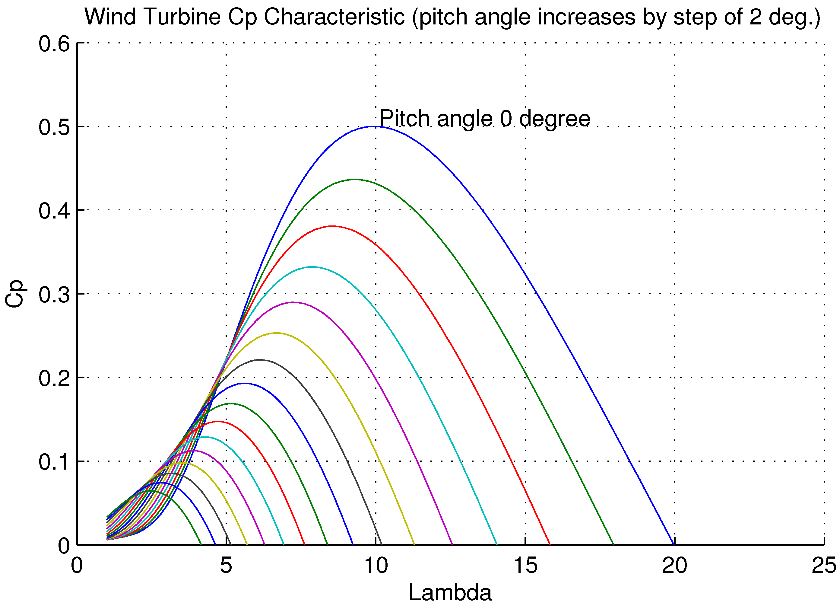
In the
Figure 3, the power coefficient,
, of the wind turbine, as a function of lambda, for different pitch angles,
β, ranging from 0 to 30 degrees is displayed. This figure shows that for
, the lambda optimum value is
, but for a larger pitch angle values the
value decreases.
Figure 3.
Turbine Power Characteristics.
Figure 3.
Turbine Power Characteristics.
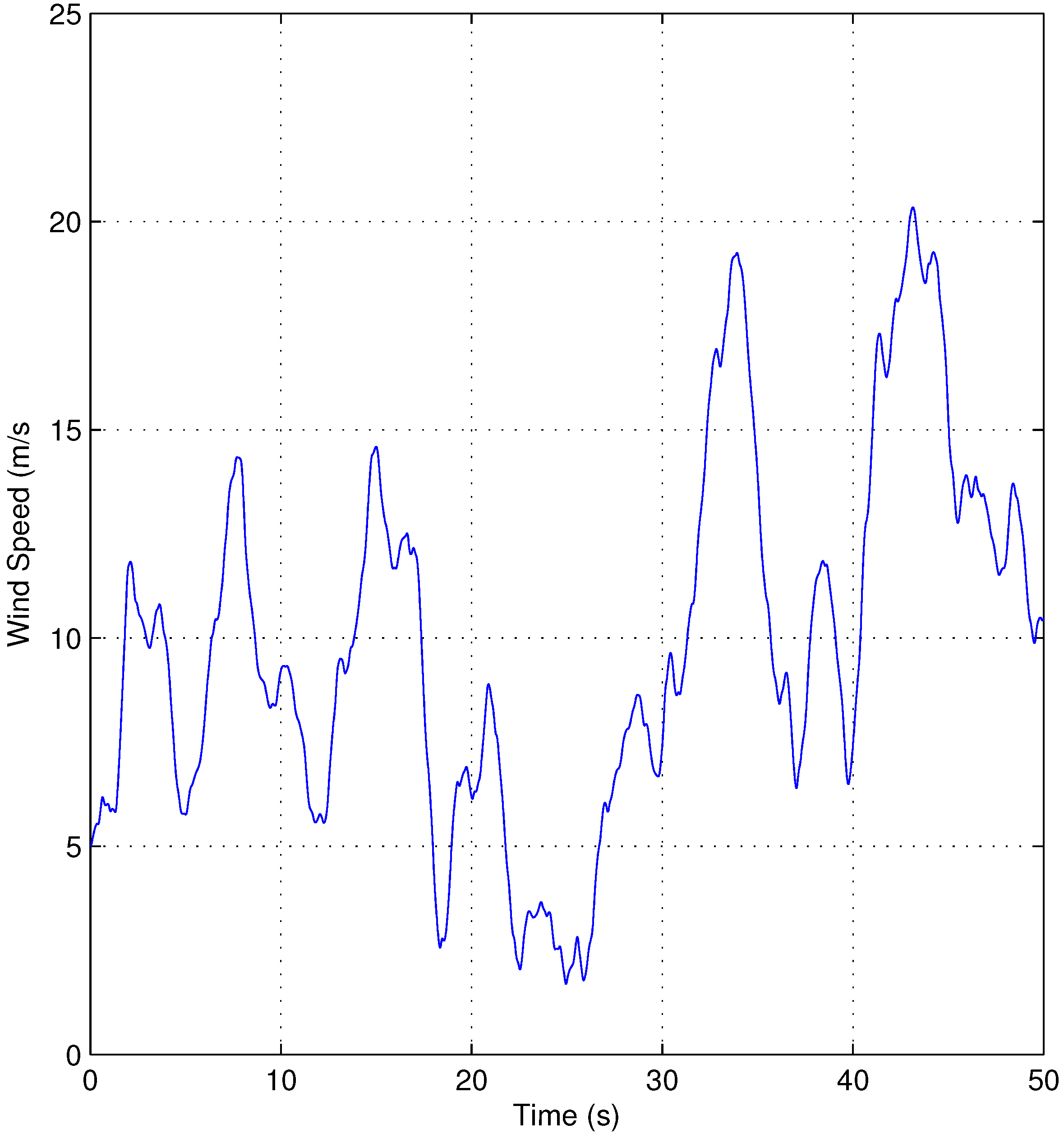
In the simulation a variable wind speed input, shows in the
Figure 4, is used. As it can be seen in the figure, the wind speed varies between 3 m/s and 20.3 m/s, and therefore the proposed controller have to maximize the electric power production for a wide range of wind speeds.
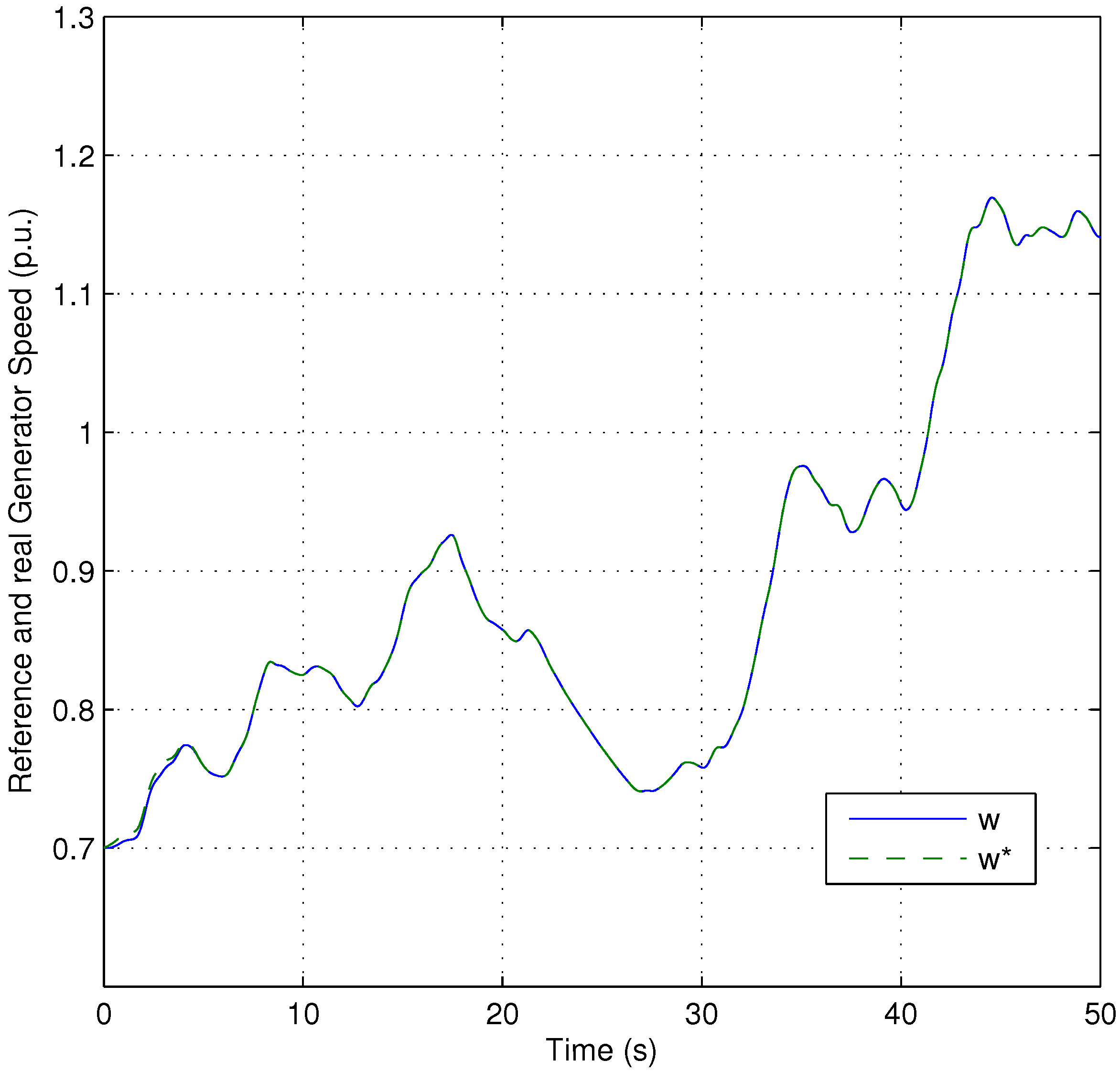
Figure 5 shows the reference (dashed line) and the real rotor speed (solid line). As it may be observed, after a transitory time, in which the sliding mode is reached, the rotor speed tracks the desired speed in spite of system uncertainties. Moreover, in this figure a good transient response can be observed because the system response do not present overshoot nor oscillations. In this figure, the speed is expressed in the per unit system (pu) that is based on the generator synchronous speed
rad/s.
Figure 5.
Reference and real rotor speed.
Figure 5.
Reference and real rotor speed.
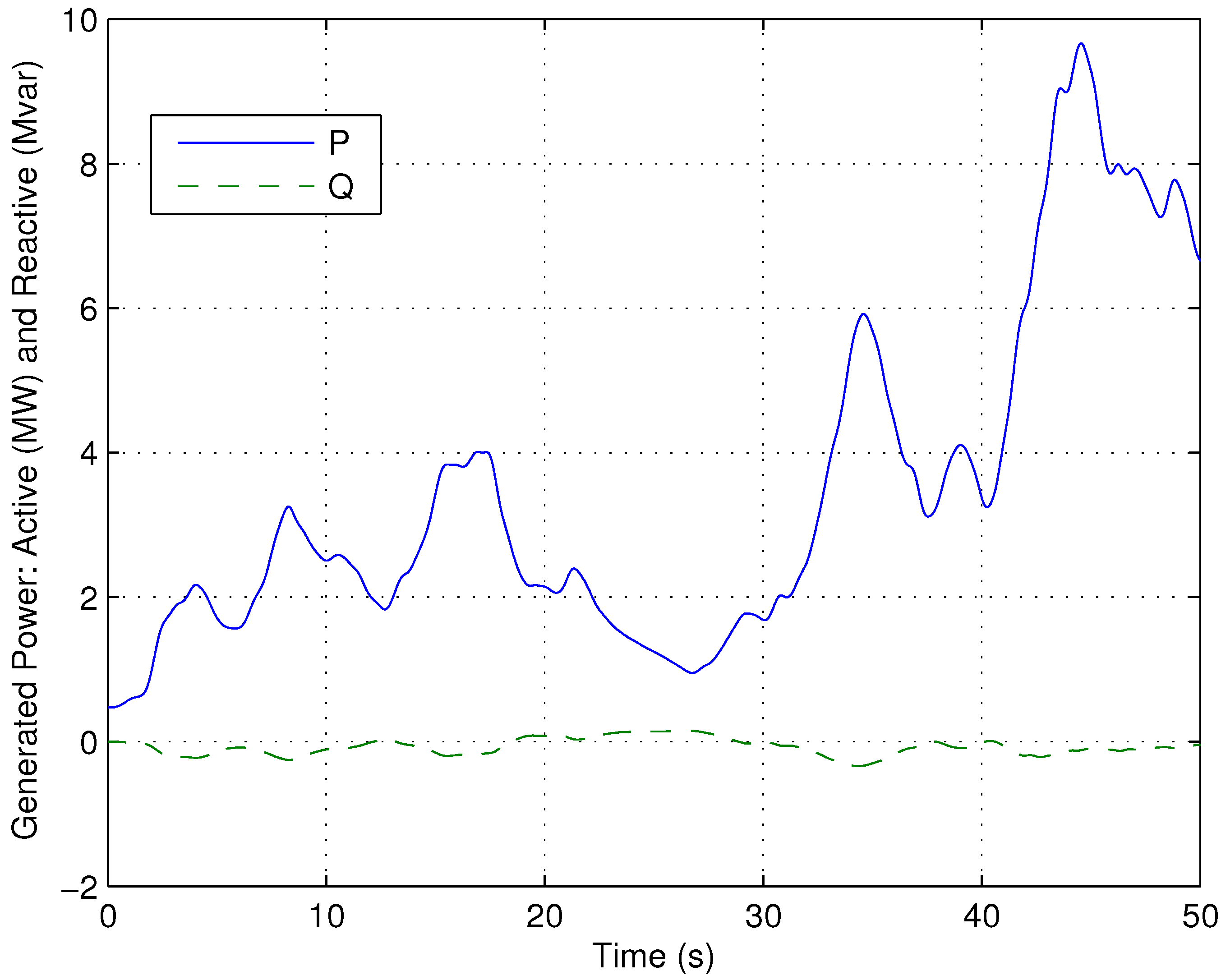
Figure 6 shows the generated reactive power (dashed line) and the generated active power (solid line), whose value is maximized by our proposed sliding mode control scheme.
Figure 6.
Generated active power.
Figure 6.
Generated active power.
Finally,
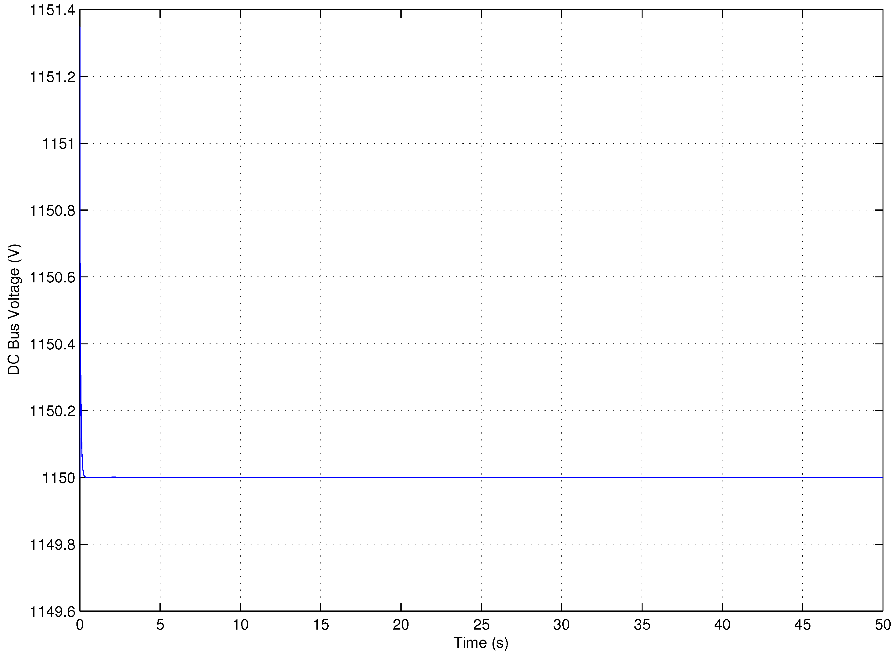
Figure 7 shows the DC link voltage response obtained using the proposed sliding mode control scheme. This figure shows that the proposed sliding mode control scheme maintains the dc-link voltage constant in spite of the system uncertainties and wind speed variations.
Figure 7.
DC Bus Voltage.
Figure 7.
DC Bus Voltage.
8. Conclusions
In this paper a sliding mode vector control scheme for a doubly fed induction generator drive used in variable speed wind power generation is described. The proposed variable structure control has an integral sliding surface to avoid the second derivative of the error signal, which is usual in the conventional sliding mode control schemes. Due to the nature of the sliding control, this control scheme is robust under uncertainties that usually appear in the real systems. The proposed control method allows to control the wind turbine operating with the optimum power efficiency over a wide range of wind speed, and therefore maximizes the power extraction for variable wind speeds.
At wind speeds less than the rated wind speed, the speed controller seeks to maximize the power according to the maximum coefficient curve. As result, the variation of the generator speed follows the slow variation in the wind speed.
The closed loop stability of the presented design has been proved through the Lyapunov stability theory.
Finally, by means of simulation examples, it has been shown that the proposed control scheme performs reasonably well in practice, and that the speed tracking objective is achieved in order maintain the maximum power extraction under system uncertainties. The simulations show that the proposed method successfully controls the variable speed wind turbine efficiently, within a range of normal operational conditions.

