Article

Factor Analysis of the Aggregated Electric Vehicle Load Based on Data Mining

State Key Laboratory of Power Systems, Tsinghua University, Beijing 100084, China
*
Author to whom correspondence should be addressed.
Energies 2012, 5(6), 2053-2070; https://doi.org/10.3390/en5062053
Submission received: 27 April 2012 / Revised: 9 June 2012 / Accepted: 19 June 2012 / Published: 21 June 2012
(This article belongs to the Special Issue Electrical Power and Energy Systems)

Abstract

:
Electric vehicles (EVs) and the related infrastructure are being developed rapidly. In order to evaluate the impact of factors on the aggregated EV load and to coordinate charging, a model is established to capture the relationship between the charging load and important factors based on data mining. The factors can be categorized as internal and external. The internal factors include the EV battery size, charging rate at different places, penetration of the charging infrastructure, and charging habits. The external factor is the time-of-use pricing (TOU) policy. As a massive input data is necessary for data mining, an algorithm is implemented to generate a massive sample as input data which considers real-world travel patterns based on a historical travel dataset. With the input data, linear regression was used to build a linear model whose inputs were the internal factors. The impact of the internal factors on the EV load can be quantified by analyzing the sign, value, and temporal distribution of the model coefficients. The results showed that when no TOU policy is implemented, the rate of charging at home and range anxiety exerts the greatest influence on EV load. For the external factor, a support vector regression technique was used to build a relationship between the TOU policy and EV load. Then, an optimization model based on the relationship was proposed to devise a TOU policy that levels the load. The results suggest that implementing a TOU policy reduces the difference between the peak and valley loads remarkably.

1. Introduction

Electric vehicles (EVs) have been promoted in recent years because of their potential to address energy security and environmental problems. It is predicted that 5.2 million EVs will have been sold worldwide by the end of 2017 [1]. This will create a great challenge. How can the power system accommodate the active, stochastic load of large-scale EV use, which might have a negative impact? Thanks to energy storage features, the grid might benefit from coordinating the charging behavior of EV owners via the potential flexibility of charging time. To reduce the negative impact and take full advantage of the positive effects, it is essential to understand the nature of the EV load from a system perspective.
Much effort has been directed toward developing an aggregated EV load model [2,3,4,5,6,7,8,9,10,11,12,13]. Since EV technology and infrastructure are still developing rapidly, it is at present difficult to construct an accurate load model. Moreover, many related issues have either not been solidified or may develop in the future. Consequently, it is interesting to determine what might happen if some important features of the aggregated EV load were to change. In other words, we are concerned how factors might affect the charging load of a swarm of EVs, such as “what is the relationship between battery size and the EV load?”, “how does the charging load curve change if the charging rate changes?”, “how does range anxiety influence the EV load if we always charge under a higher state of charge (SOC)?” and “what type of time-of-use (TOU) pricing policy will shift the EV load?” All these questions can be evaluated based on a factor analysis of the aggregated EV charging load.
Several studies have investigated the impact of factors on EV load [2,3,4,14]. Some assessed the impact of the charging rate, battery size, and penetration of the charging infrastructure on the EV load by constructing load curves [3,4]. Others assessed the effects of a given TOU policy on the load profiles with EV penetration [2,14]. Briefly, previous studies evaluated mainly the qualitative impact of some factors. However, it is also important to assess the quantitative impact of these factors on the aggregated EV load at a given instant. For instance, it is crucial to know how much the EV load changes with the factors. The impacts of different factors on the EV load should also be compared. Besides, a precise TOU policy needs devising to coordinate the EV aggregated load. These quantitative impacts haven’t been studied in detail and will be discussed here. In this study, the accurate temporal impact of each factor can be determined by means of a quantitative assessment. Based on the results, the aggregated EV load might be regulated by adjusting the values of controllable factors as well, such as by devising a TOU policy.
In order to quantify their impact on the EV load, we classified the factors as internal and external. The former include the battery size, charging rate selected by owners in different locations, penetration of the charging infrastructure, and charging habits. The latter mainly refers to the TOU policy. Data mining techniques were used to build the model by analyzing numerous EV load profiles for different values for these factors. The quantitative relationship between the EV load and these factors can be captured by linear regression (LR) and support vector regression (SVR) with massive input data. However, such input data does not exist in the real world, due to the relative scarcity of EVs and because the values of some factors are fixed. Consequently, a simulation is necessary to generate the input data.
Many studies have concentrated on prediction of the EV load profile by simulation [2,3,4,5,6,7,8,9,10,11,12,13]. A growing number of investigators have adopted specified real-world travel datasets to model the EV charging load, such as the National Household Travel Survey (NHTS) [15]. This real-world travel dataset includes the historical travel information of 150,147 households, including the number of daily trips, and the start and end times, distance, and purpose of each trip. Exploiting this travel dataset, two approaches can be used to predict the EV load: an indirect or stochastic approach and a direct or deterministic approach [13]. Both approaches are first used to simulate the daily EV travel schedules, and the charging schedules can be made based on the results. The difference between the two approaches is in the simulation of travel schedules. Using the indirect approach, travel information (such as the daily mileage) is calculated using probability distributions, rather than extracting it from the travel dataset directly [11,12,13]. The probability distribution of the travel information is fit by the statistics in the dataset. Using the direct approach, the daily trip schedule of an EV is considered to be identical to the vehicle information in the travel dataset, and the travel schedules of the total EV swarm are simulated exactly in accordance with the data records in the travel dataset [2,3,4,8]. We adopted the direct approach to generate different EV loads as data mining input.
The remainder of the paper is organized as follows: Section 2 proposes the framework of the data mining-based modeling. The methodology used to generate the data mining input data is shown in Section 3. Section 4 uses linear regression to model the relationship between the EV load and the internal factors, and evaluates the impact of these factors on the charging load. In Section 5, SVR modeling is used to build a relationship between the EV load and external excitation, which is the instant when the price of electricity changes. Section 6 presents our conclusions.

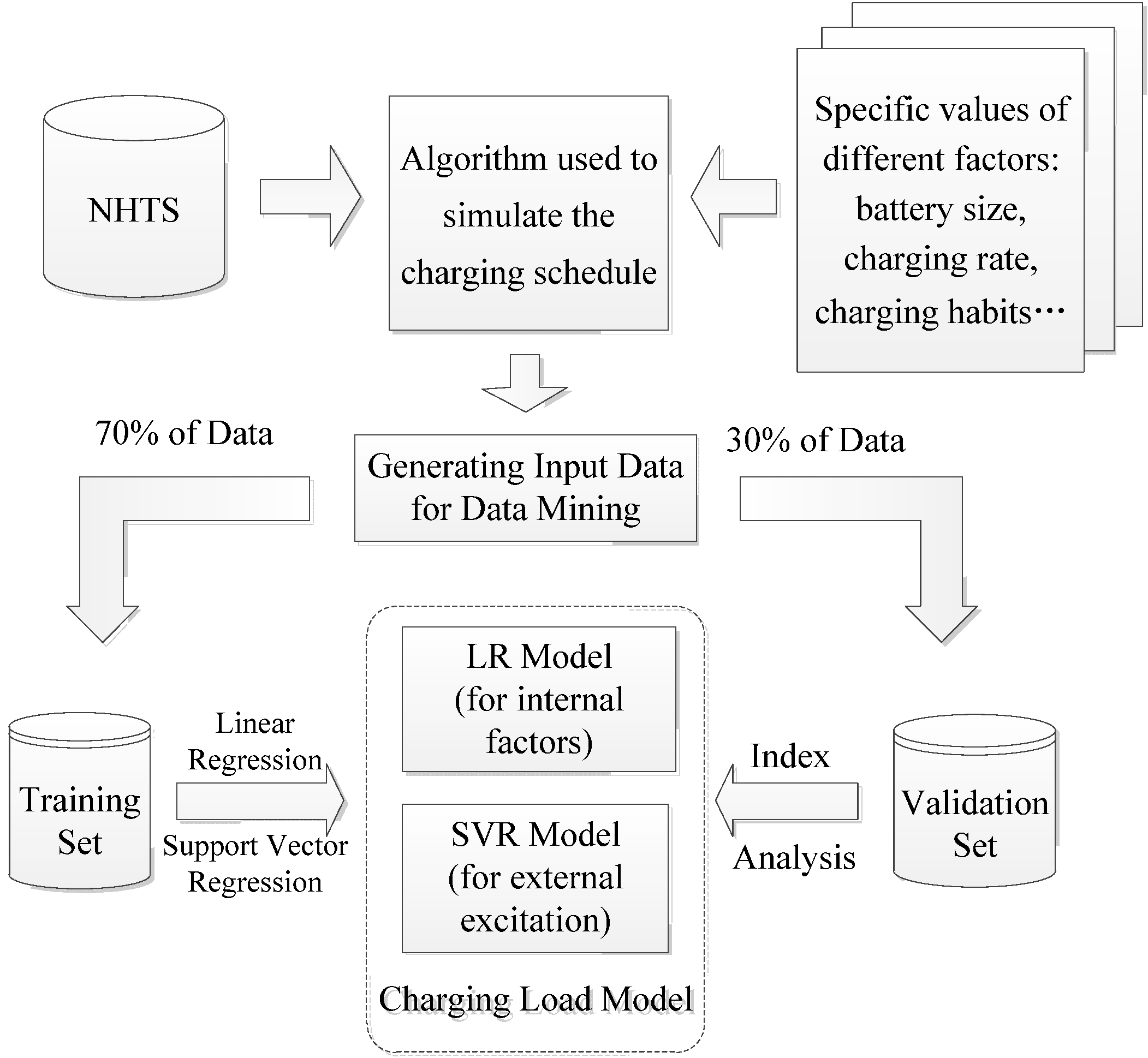
2. Framework of Data-Mining Based Modeling

Data mining (DM) techniques are adopted to examine the relationship between the EV load and various factors. The framework of the DM technique is shown in Figure 1. Data mining is always based on a massive input dataset. Since the input data in this case are unavailable in the real world, the first step of modeling is to generate large amounts of simulation data as input; the data describe the different EV load profiles for different values of the important factors to be investigated. The simulation adopts a direct-approach-based algorithm, in which a real-world travel survey serves as the background data to ensure that the simulation is consistent with the travel patterns of EV owners. Seventy percent of the input data is used as the training set, while the rest serves as the validation set.
The second step is to build the relationships between the EV load and the factors analyzed. LR is used to build the relationship between the EV load and the internal factors, because the LR coefficients represent the sensitivity of the EV load to these factors. SVR is appropriate for modeling external excitation, i.e., the instant when the price of electricity changes. With this model, a TOU policy can be devised to achieve the expected EV load, which is essential for load leveling.
Figure 1. Framework of DM-based modeling.
Energies 05 02053 g001
The third step is to validate the models. Two methods for validating the models are proposed: one calculates the model error using an index and the other analyzes the stability of the model coefficients.

3. Generating Input Data by Simulation

3.1. Methodology

The charging load of every EV at a given instant is assumed to be an independent random variable that follows the same probability distribution. According to the Central Limit Theorem, when n is a very large number, the EV load follows the normal distribution [3]:
i = 1 n P i ( t ) ~ N ( n μ ( t ) , n σ 2 ( t ) )
where n is the total number of EVs; Pi(t) denotes the load of the ith EV (i=1,2,…,n) in time step t; and µ(t) and σ2(t) are the expectation and variance of Pi(t), respectively. As long as the parameters µ(t) and σ2(t) are identified, the EV load can be predicted from Equation (1). These parameters can be calculated using the following method. When m is a large number, the law of larger number (LLN) suggests that:
μ ( t ) = 1 m i = 1 m P i ( t )
In addition, according to the aforementioned assumptions and the LLN:
σ 2 ( t ) = 1 m i = 1 m P i 2 ( t ) μ 2 ( t )
From Equations (2) and (3), the EV load profile can be generated from the charging schedules (P1(t), P2(t), …, Pm(t)) (m is a large number).

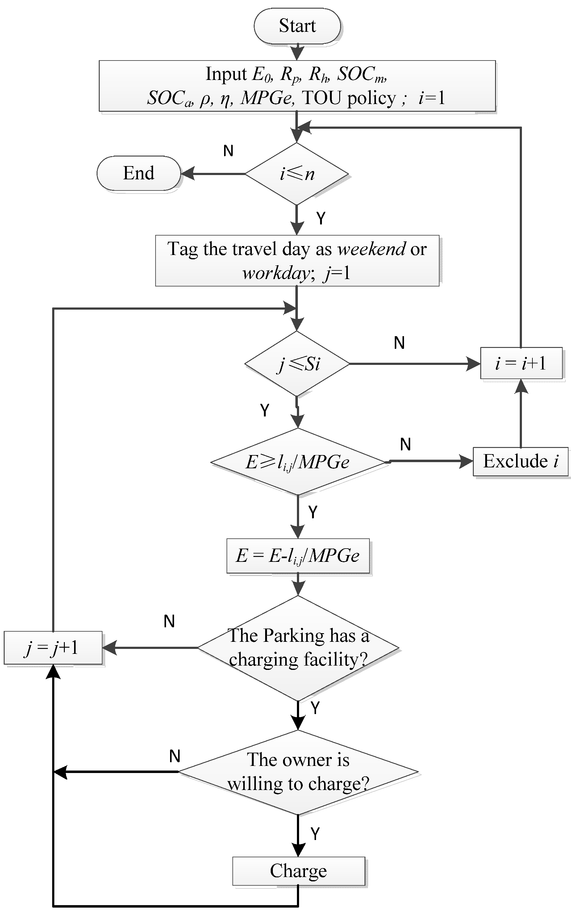
3.2. Simulation of the Charging Schedules

In order to predict the EV load, one must know the charging schedules. Assume that the travel behavior of EVs is identical to that of conventional vehicles (CVs). This assumption is acceptable when CVs are replaced by EVs and the performance of EVs is satisfactory in future. Consequently, an algorithm using the direct approach is developed to simulate the charging schedules based on the historical travel information for CVs. The historical travel information for each CV can be extracted from the NHTS. Since current commercial EVs are mainly cars, only vehicles labeled “CAR” are selected from the NHTS for the charging schedule simulation. If necessary, vehicles of other types can also be used in the simulation using the same methodology. In addition, the algorithm considers the factors associating with charging EVs mentioned in Section 1, as shown in the Table 1.
Table 1. Variables used in the algorithm to simulate the charging schedules.
Variable NameVariable Description
E0EV battery size
RpCharging rate in public places
RhCharging rate at home
SOCmSOC threshold related to battery maintenance
SOCaSOC threshold related to range anxiety
ΡPenetration of public charging infrastructure
MPGeMiles per gallon of gasoline equivalent
tupInstant when the price of electricity increases
tdownInstant when the price of electricity decreases
ηEfficiency of the charger
SOC0SOC for the first trip
nTotal number of vehicles in the simulation
iEV no.
jTrip no.
ECurrent energy stored in the battery
SiTotal number of the trips by EVi
li,jMileage of trip j for EVi
The following three assumptions are made. First, the study considers a simple TOU policy, in which only two price signals are sent at different times in one day to divide it into two periods: the periods with regular and reduced electricity prices. tup and tdown are the instants when the price of electricity increases and decreases, respectively. A more sophisticated TOU policy can be studied in future work. Second, the charging power is constant. The charging load of an EV is r kW, while the charging power to the battery is ηr, where r is the charging rate of the charger and η is the efficiency of the charger. Here, η = 0.9. Finally, the mileage per unit of electrical energy is 3.042 mi/kWh, which is the value for the Nissan Leaf [16].
The algorithm used for simulating the charging schedules is shown as Figure 2. In order to generate reasonable charging schedules and reduce the influence of an inappropriate starting SOC assumption, the EV follows the same daily travel schedule for three consecutive days. The starting SOC of the first trip on day one is 100%. The charging schedules of days two and three are stored as the results.
First, the daily travel schedule of vehicle i is read and the travel day is tagged as a workday or a weekend day. Considering the significant differences between the travel patterns on workdays and weekends, the charging schedules generated for workdays and weekends are used separately in modeling.
Second, the algorithm reads the information for trip j of EV i. If the current energy E will enable the distance of trip j, the energy used for the trip will be consumed. Then, the algorithm judges whether a charging service is available at the location where trip j ends. Charging infrastructure is assumed to be always available at home, while the infrastructure in a public place may be limited, such as at workplaces, shops, restaurants, and places for medical or dental service. The probability that a public place offers a charging service is denoted as ρ ( ρ [ 0 , 1 ] ). In other places, there is no charging infrastructure.
Figure 2. Algorithm used for generation of charging schedules.
Energies 05 02053 g002
Third, when a charging service is available, the algorithm judges whether the owner of the EV is willing to charge the EV. This willingness depends on the SOC. When the SOC is in the interval [SOCm, 1], the owner will not charge to maintain the battery. When the SOC is in the interval [0, SOCa], the owner must charge because of range anxiety. When the SOC is in the interval [SOCa, SOCm], the probability that the owner charges the EV is set as 0.5. The combination of SOCm and SOCa characterizes the owner’s charging habit.
Finally, the target of charging is to reach the highest possible SOC before the next trip. When this target can be achieved, the lowest electricity cost is pursued. However, if the owner has multiple potential charging schedules that can all charge the battery pack fully, while paying the same lowest electricity price, the charging schedule is selected randomly.

4. Internal Factors Analysis

4.1. Purpose and Method

A linear regression model was developed to quantify the impact of internal factors on the EV load. From Section 2, the expectation of the EV load can be calculated using n and µ(t). As a result, the estimate of µ(t) is chosen as the output of the LR model, which is denoted as μ ^ ( t ) . The internal features are the inputs of the model. Therefore, μ ^ ( t ) is expanded as μ ^ ( F , t ) , where F represents the vector of the internal factors. The coefficients of the factors can be used to quantify the impacts. With plenty of input data (F,t) and µ(F,t), the LR model can be built:
μ ^ ( F , t ) = k = 1 6 b ^ k ( t ) F ( k ) + b ^ 0 ( t )
where F represents the vector of factors, i.e., (E0, Rp, Rh, SOCm, SOCa, ρ); t is the time step; k is the number of factors in F, and b ^ k is the coefficient estimate gained by the LR (k=0,1,…,6). Note that no TOU policy is implemented here when generating massive simulation data as input. The values of the variables can be generated randomly and the corresponding µ(F,t) can be computed by simulation. Using the same approach, models are built for workdays and weekends with separate training data.

4.2. Implementation

A 96-point curve was adopted to describe the EV load for one day, i.e., each time step is 15 minutes. For each time step, the factors are sampled randomly according to the range in Table 2 and 100,000 simulation samples are generated with different factor values. First, 70,000 samples are selected as the training set, while 30,000 samples serve as the validation set (data for the 3rd travel day).
Table 2. The bounds used for factor sampling.
VariableLower boundUpper bound
E0 (kWh) *1635
Rp (kW) **1.47.7
Rh (kW)1.47.7
SOCm (%)50100
SOCa (%)050
ρ (%)0100
* The battery sizes of the Chevrolet Volt and MINI E are chosen as the bounds [17,18]; ** The range of charging rates is from [19].
Although all of the factors affect the EV load, some factors may prove insignificant for a specified time step. Therefore, the stepwise regression technique was used to select the significant factors and corresponding coefficients [20]. Furthermore, the values of the factors were normalized according to their upper and lower bounds, in order to compare the significances of different factors using the coefficients.
After the regression, the coefficients b ^ k ( t ) are calculated (k = 0,1,…,6; t = 1,2,…,96). Here, t = 1 represents the time step from 0:00 to 0:15, and so on. For a given tp, the coefficient b ^ k ( t p ) represents the sensitivity of the EV load to that factor. The coefficient of each factor can be used to evaluate its impact on the EV load. If the coefficient is positive, the EV load increases with the value of the factor, and vice versa. In addition, the value of the coefficient quantifies the contribution of the factor to the EV load. For instance, from 18:00 to 18:15 (the 73rd time step), the load model can be expressed as:
μ ^ ( F , 73 ) = 0.0583 E 0 0.0110 R p + 0.419 R h + 0.0996 S O C m + 0.315 S O C a 0.0500 ρ + 0.259
Considering factor Rh, if the charging rate increases 1 kW, the average EV load increases 0.0665 kW [0.419 × 1 kW/(7.7 − 1.4)] from 18:00 to 18:15.
For a given Fp, μ ^ ( F p , 1 ) , μ ^ ( F p , 2 ) , ... , μ ^ ( F p , 96 ) is the estimated power demand of the EVs throughout an entire day for the specified internal factors. For example, take Fp = (24, 6, 2, 90, 50, 50) (E0 = 24 kWh, Rp = 6 kW, Rh = 2 kW, SOCm = 90%, SOCa = 50%, ρ = 50%). Figure 3 shows the results for μ ^ ( F p , t ) (t = 1,2,…,96), showing the real average EV load profile based on the simulation (in red) and the estimated average EV load profile from the regression Model (4) (in blue). The estimated model is accurate enough to approximate the real one.
Figure 3. The real and estimated average EV loads.
Energies 05 02053 g003

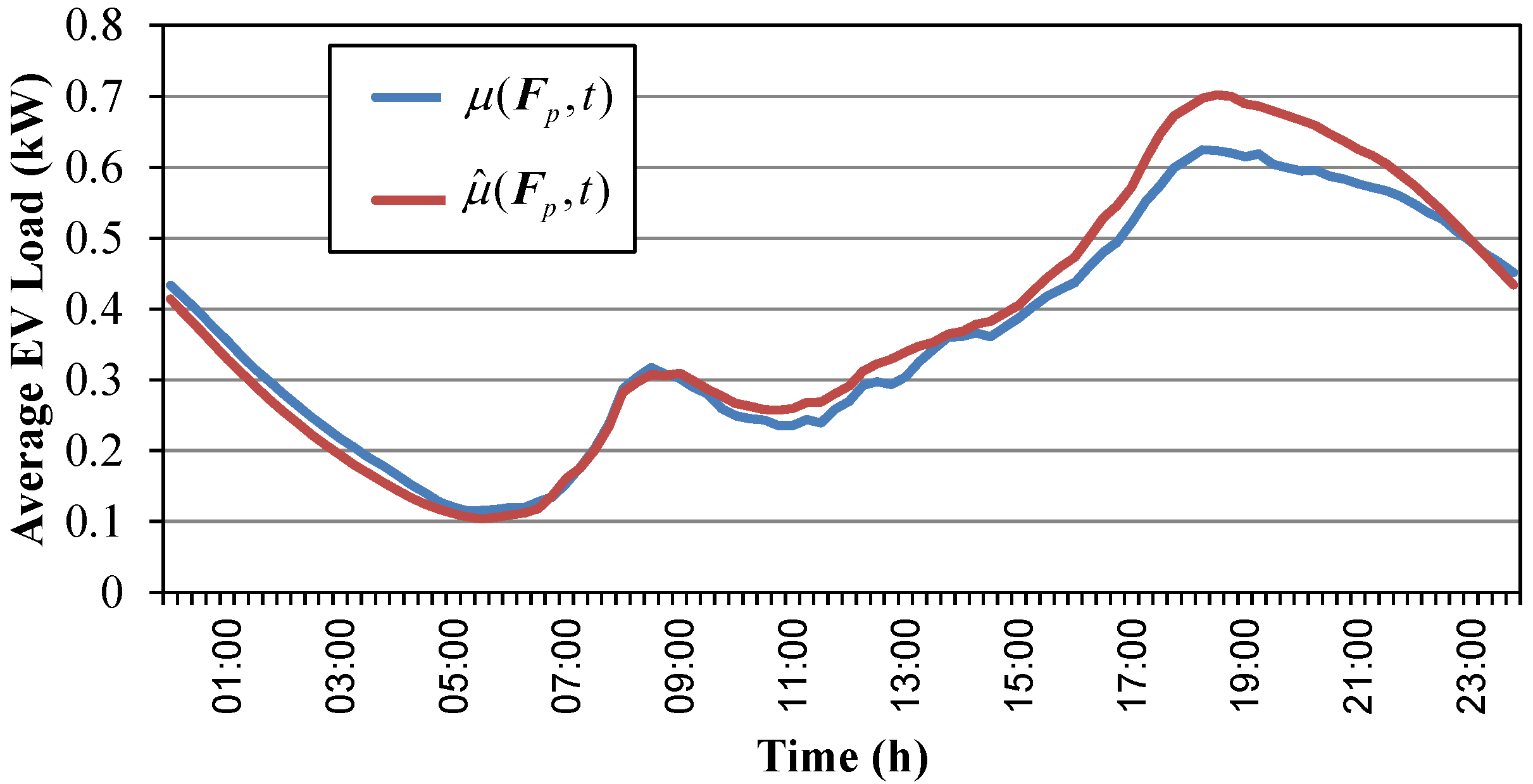
4.3. Model Validation

The Mean Energy Error (MEE) was adopted to validate the model using the data in the validation set:
M E E = 1 i = 1 t T | μ ^ i Δ t μ i Δ t | t T μ i Δ t
where i is the number of the EV load profile in the validation set; is the total number of EV load profiles in the validation set; ∆t is the length of the time step (15 minutes); and T is the set of all time steps in a day. The MEE describes the mean error of the estimated charging energy demand during a day compared to the real values in the training set. As the charging energy is calculated using the EV load and length step, the MME can represent the error of the estimated EV load.
The MEEs for workdays and weekends are 10.25% and 9.41%, respectively, which are acceptable for analyzing the relationship between the EV load and the internal factors.

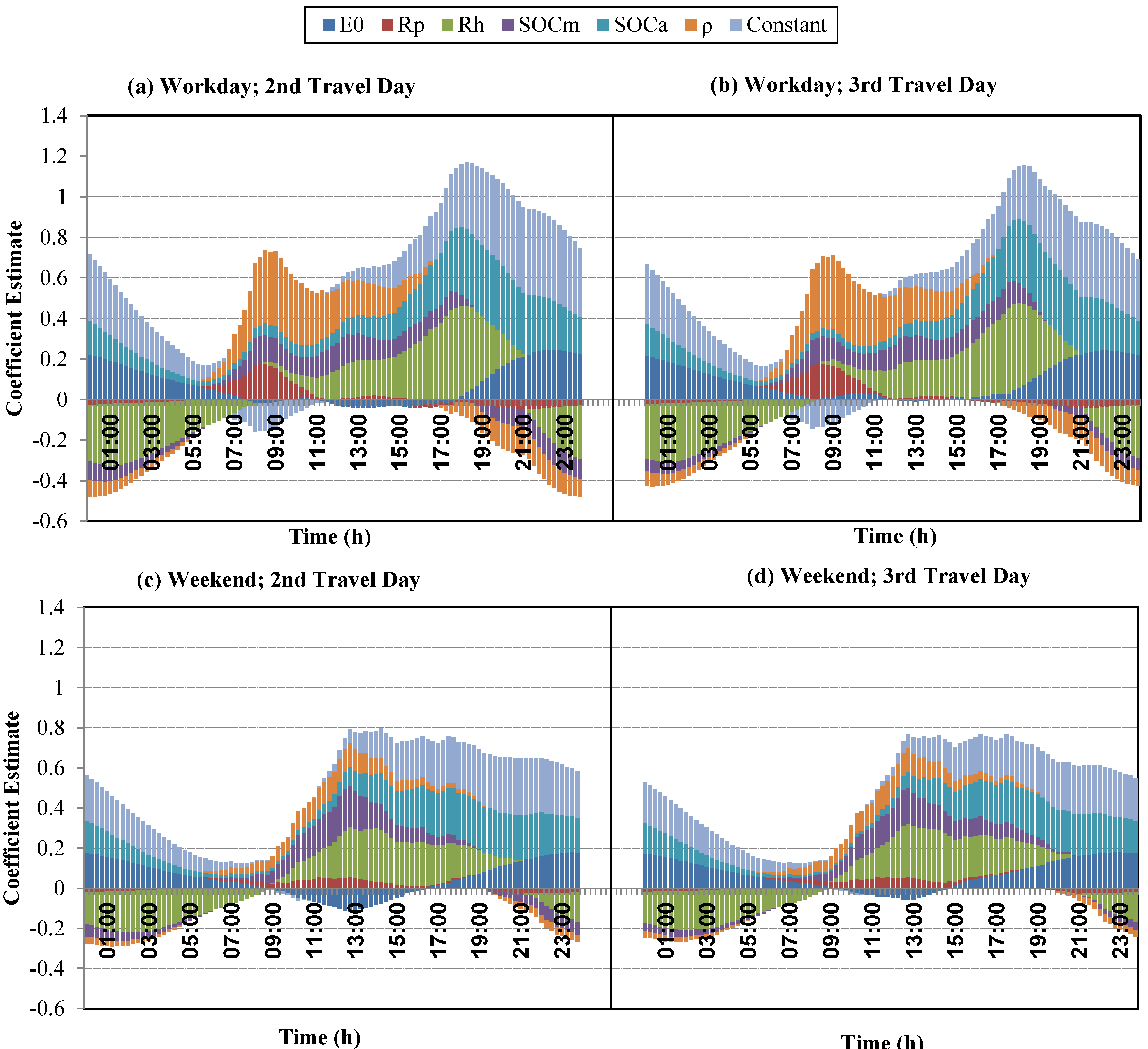
4.4. Observations and Discussion

The charging profiles for the second and third days are used and stacked graphs of the regression coefficients are shown in Figure 4.
Figure 4. Stacked graphs with the regression coefficients of the internal factors. Workdays with the input data for the (a) 2nd and (b) 3rd travel day; Weekends with the input data for the (c) 2nd and (d) 3rd travel day.
Energies 05 02053 g004
In the stacked charts of the regression coefficients, different factors are shown in different colors. There are seven columns at each time step and the length of a column in one color denotes the absolute value of the factor’s coefficient at that time step. If the column is above the time axis, the factor is positively correlated with the EV load at that time step and vice versa. Therefore, the impacts of all of the factors on the EV load in one time step can be investigated by analyzing the lengths and positions of the columns in different colors at one time step. In addition, the impact of one factor throughout a day can be evaluated by observing the columns in the corresponding color at all time steps. Note that if the absolute value of the coefficient is greater than 0.05, the impact of the factor is considered major.
Comparison of Figure 4(a) and 4(b), as well as comparison of Figure 4(c) and 4(d), shows that the contribution of each coefficient of the factor stays approximately the same on different travel days, which validates the stability of the model. The internal factors are analyzed in detail below.

4.4.1. Battery Size

An EV with a larger battery travels farther. However, traveling a longer distance requires more electrical energy. Therefore, a larger battery leads to a greater energy demand. The stacked chart can determine when the increased energy demand will be met.
On workdays, the coefficient is greater than 0.05 from 18:00 to 6:00 the next day, which indicates that a larger battery leads to a higher EV load for that interval. It can be inferred that the increment in energy consumed caused by the larger battery size is supplied at night (18:00 to 6:00 the next day). Similarly, the energy increment occurs from 16:30 to 6:00 the next day on weekends.

4.4.2. Charging Rate in Public Places

Figure 5 shows that many EVs are parked in public places from 7:00 to 17:00. According to the analysis of the coefficient in Figure 4, Rp significantly influences the EV load only from 7:00 to 10:30, and not 7:00 to 17:00. This phenomenon can be explained as follows. After 7:00 on workdays, many EVs arrive at workplaces from home. As travel to the workplaces consumes energy, some owners are willing to charge when EVs are parked. However, the energy demand of these EVs is not large, because most EVs start from home with a high SOC. Therefore, most EVs parking in public places can finish charging before 10:30, and so the charging rate will not significantly affect the EV load from 10:30 to 17:00.
Figure 5. Total number of EVs parking in public places at each instant: (a) workdays; (b) weekends.
Energies 05 02053 g005
On weekends, the coefficient of this factor is greater than 0.05 from 11:30 to 13:00, which indicates the EV load increases with ρ during this period. An analysis similar to that for workdays may be performed.

4.4.3. Charging Rate at Home

Regarding the time step t and a given Rh, two groups of EVs contribute to the EV load at t: the EVs that parked before t that have not finished charging and the EVs arriving at home at t to start charging (Figure 6). On the one hand, as the energy demand of the first group of EVs is limited, when Rh increases, an increasing number of EVs in the first group can finish charging before t. Therefore, the power demand of the first group at t is reduced as Rh increases. On the other hand, for the second group of EVs, the power demand increases with Rh. It is interesting to determine how the total power demand of EVs changes with Rh. Figure 4 shows that as Rh increases, the EV load increases from 10:00 to 20:30 and decreases from 21:30 to 7:00. Let ∆n1(t) denote the total number of EVs that finish charging before t due to the increase in Rh, and ∆n2(t) denote the total number of the EVs in the second group. It can be concluded that from 10:00 to 20:30 ∆n1 is always smaller than ∆n2, while from 21:30 to 7:00, ∆n1 is always greater than ∆n2. For weekends, a similar analysis can be performed.
Figure 6. Total number of EVs arriving at home at each instant: (a) workdays; (b) weekends.
Energies 05 02053 g006

4.4.4. Battery Maintenance

If the owner is concerned with the lifetime of the EV battery, he will charge his EV less frequently, which results in a lower power demand during this period. Nevertheless, he has to charge his EV during another period when the SOC is too low. The power demand is higher in this period due to the lack of charging in the previous period. From the analysis of the coefficient of SOCm shown in Figure 4, the two periods can be identified.
On workdays, the EV load increases with SOCm from 6:00 to 19:30, while the trend is opposite in the other period. A lower SOCm means caring about the battery more. Therefore, from 6:00 to 19:30 the owners charge their EVs less frequently due to battery maintenance, the approximate period that compensates for this amount of energy is from 19:30 to 6:00 the next day. According to a similar analysis, on weekends fewer EVs are charged from 6:30 to 21:00, and the “compensating” period is from 21:00 to 6:30 of the next day.

4.4.5. Range Anxiety

Throughout the day, the coefficient of this factor is positive, which indicates that the power demand increases with SOCa. The higher SOCa is, the more the owner suffers range anxiety. The phenomenon shows that throughout the day, the more the owner suffers from range anxiety, the greater the power demand of the EV is, since the owners tend to keep the SOC higher. These owners can finish longer trips in their EVs, but their EVs require more energy, increasing the power demand. There is no clear difference in this phenomenon on workdays and weekends.

4.4.6. Penetration of the Public Charging Infrastructure

As ρ increases, more EVs parked in public places can be charged if necessary, typically in the daytime. Therefore, more power is required in the daytime when ρ increases. However, if more energy is supplied in the daytime, then less energy is supplied during other periods, which means that less power is demanded during those periods with increasing ρ. The analysis of the coefficient of ρ on workdays showed that if ρ increases, the EV load increases from 5:30 to 17:00 and decreases during other periods. Similar analysis can be carried out for weekends.

4.4.7. Critical Factors

The relative coefficients of the aforementioned factors were analyzed to compare their significance and identify the critical factors. The relative coefficient of the kth factor is defined as:
b ^ k % ( t ) = b ^ k / k G | b ^ k | × 100 %
where G is the set of all the internal features. The relative coefficient represents the relative contribution of that factor at a given time step. When the absolute value of the relative coefficient at a time step is greater than 30%, the corresponding factor is considered a critical factor in that time step. The critical factors at each time step are shown in Figure 7. If the EV load and the critical factor are positively correlated, then the factor is called a positive critical factor; otherwise, it is called a negative critical factor.
Figure 7. The critical factors at each time step: (a) Workdays; (b) Weekends.
Energies 05 02053 g007

5. Analysis of External Excitation

5.1. Purpose and Method

To devise a suitable TOU policy, it is also important to know how the EV load profile responds to the price of electricity. This paper considers the instants when the price of electricity changes, from high to low or the reverse. It does not consider what prices to set.
Naturally, the relationship between the EV load and the instants when the price of electricity changes is highly nonlinear. Experiments proved that the error of the model describing this relationship is unacceptable when it is built using linear regression. Therefore, SVR was adopted for modeling the relationship between µ and (tup,tdown). The estimate of µ(t) is chosen as the output of the SVR model, which is denoted as μ ^ ( t ) . As the influence of price signals is to be investigated, μ ^ ( t ) is expanded as μ ^ ( t u p , t d o w n , t ) .
Here we provide a brief introduction to SVR. With much training data ( x 1 , y 1 ) , ( x 2 , y 2 ) , ... , ( x , y ) , an SVR model can be built that describes the relationship between the target y and the feature vector x [shown in Equation (8)], where y ^ is the estimate of y. The SVR ensures that most training errors are within the given error and the regression function fits the unknown data best. However, some parameters have to be selected for SVR modeling, such as the tolerance of the training error for most training data ε, the tradeoff between the ability to predict unknown data and the tolerance for the training error, which is larger than ε (denoted as C) and the kernel function k ( x i , x j ) :
y ^ = i = 1 ( α i α i * ) k ( x i , x ) + b
The approach used to select the parameters is as follows. First, the kernel function is selected from classical functions, such as the radial basis function (RBF) k ( x i , x j ) = e γ x i x j 2 . Then, ε can be identified after trials, as long as the performance of the SVR is sufficient. Lastly, only the parameters of the selected kernel function (such as γ of the RBF) and C should be identified. N-fold Cross Validation and Grid Search can be used to search for the proper parameters [21].
After selecting the parameters, the model can be established by calculating coefficients αi, αi * and b for equation (8) (i = 1,2,…, ). An optimization problem is solved to compute the coefficients of the SVR model [22]:
max α i , α i *   { 1 2 i , j = 1 ( α i α i * ) ( α j α j * ) k ( x i , x j ) ε i = 1 ( α i + α i * ) + i = 1 y i ( α i α i * ) subject to i = 1 ( α j α j * ) = 0   and   α i , α i * [ 0 , C ]
In our study, y is µ and x is (tup, tdown, t). RBF is chosen as the kernel function, and then the charging load model can be expressed as:
μ ^ ( t u p , t d o w n , t ) = i = 1 ( α i α i * ) e γ ( t u p i , t d o w n i , t i ) ( t u p , t d o w n , t ) 2 + b
With this model, the relationship between the EV load and TOU policy can be established. For example, for a given TOU policy ( t u p A , t d o w n A ), the estimated EV load at time step t can be calculated by inputting ( t u p A , t d o w n A , t) into Equation (10). Using this method, the daily EV load with the implementation of a given TOU policy can be determined. Conversely, for a given daily EV load, a TOU policy ( t u p B , t d o w n B ) can also be made using Equation (10). The case studies in the next section present an application for making a TOU policy.

5.2. Case Studies

An SVR model was built to develop a TOU policy for load leveling. The purpose of the TOU policy is to shift the EV load to the original load valley. The TOU policy was made for a province in China on a summer workday. The load profiles without EV integration are collected and called the base load. The peak load of the province is about 6,800 MW. Assume that the total number of EVs is one million and that all the EVs respond to the TOU policy, which is a best-case scenario. In addition, the grid infrastructure is capable of handling many EVs. The problem can be formulated in a way similar to that in [23]. In [23], however, the variable is the charging schedule, while here it is the timing of the price signals:
min t u p , t d o w n   V = 1 L t = t α t β [ n μ ^ ( t u p , t d o w n , t ) + L 0 ( t ) L ] 2 subject   to { L = 1 t β t α t = t α t β [ n μ ^ ( t u p , t d o w n , t ) + L 0 ( t ) ] , t T μ ^ ( t u p , t d o w n , t ) = i = 1 ( α i α i * ) e γ ( t u p i , t d o w n i , t i ) ( t u p , t d o w n , t ) 2 + b ,   t T
where n is the total number of EVs; L0(t) is the base load of the province; and L indicates the average power for a day. The meanings of the other symbols are given above.

5.3. Implementation of SVR Modeling and Model Validation

Before resolving Equation (11), the model shown in Equation (10) has to be built. The training data for modeling can be obtained as follows: the value of (tup, tdown) is generated randomly after the values of the vector (E0, Rp, Rh, SOCm, SOCa, ρ) are assigned. In the case studies, the assigned value is (24, 6, 2, 90, 50, 50). Then, the corresponding µ(tup, tdown, t) can be computed using the methodology in Section 3. First, 10,080 pairs of µ(tup, tdown, t) and (tup, tdown, t) are selected as the training set, while 4,320 pairs serve as the validation set (data for the 3rd travel day). The length of each time step is 15 minutes.
After acquiring the training data, the parameters can be selected and the coefficients in Equation (10) can be calculated using the methods mentioned above, thanks to LIBSVM [21]. Therefore, the SVR model in Equation (10) can be established.
The MEE shown in Equation (5) was also selected as an index for validating the SVR model using the data in the validation set. The MEE for workdays was 16.89% (each time step was 15 minutes), demonstrating that a relationship between the EV load and price signal can be built with the SVR approach. If LR is used to build this model, the MEE is 37.11%, which is unacceptable.

5.4. Results

Since problem Equation (11) is difficult to solve with conventional algorithms, an intelligence-based technique called particle swarm optimization (PSO) is used to solve the problem. Kennedy and Eberhart were inspired by flocking birds and introduced PSO in 1995 [24,25]. The particle swarm optimization toolbox, PSOt, is used to solve Equation (11) [26]. However, some parameters remain to be identified. An acceptable set of parameters is attained after experiments.
The solved inexpensive period is from 23:45 to 4:45. The EV load is shifted significantly to the off-peak period of the base load (Figure 8). The results of the total load and peak-valley difference are shown in Figure 9, comparing three scenarios: (S1) the base load; (S2) the total load without a TOU policy; and (S3) the total load with a TOU policy.
It is obvious that when EVs are introduced without a TOU policy, the load profile is worse because of the increased load variance and peak-valley-load difference. With a TOU policy, the difference between the peak and valley is reduced by 39.11%. These results demonstrate that the load profile improves remarkably with a TOU policy using our SVR model.
Figure 8. EV load profiles with and without implementation of a TOU policy.
Energies 05 02053 g008
Figure 9. (a) Total load for different scenarios; (b) Difference between the peak and valley with different scenarios.
Energies 05 02053 g009

6. Conclusions

Considering real-world travel patterns by exploiting the NHTS, a framework based on data mining is proposed for modeling the aggregated EV load. A linear load model is developed for the internal factors, with which the character and temporal distribution of the coefficients can be used to evaluate the impacts of the internal factors on the EV load quantitatively. Furthermore, a relationship between the EV load and external excitation is built; based on this, an optimization model is used to devise a TOU policy for load leveling. In the future, further research on TOU is planned, which will examine not only when to change the price of electricity, but also how to set the price.

Acknowledgments

This work was supported by the MOST (Ministry of Science and Technology) of China (No.2010DFA72760), National Science Fund for Distinguished Young Scholars (51025725) and Tsinghua University Initiative Scientific Research Program.

References

  1. Cowan, L.K. 5.2 million strong: Report predicts 46× increase in EV sales by 2017. Inhabitat. 24 August 2011. Available online: http://inhabitat.com/5-2-million-strong-report-predicts-46x-increase-in-ev-sales-by-2017/rsz-pike-research-ev-sales-predictions-chart (accessed on 14 March 2012).
  2. Darabi, Z.; Ferdowsi, M. Aggregated impact of plug-in hybrid electric vehicles on electricity demand profile. IEEE Trans. Sustain. Energy 2011, 2, 501–508. [Google Scholar] [CrossRef]
  3. Wu, D.; Aliprantis, D.C.; Gkritza, K. Electric energy and power consumption by light-duty plug-in electric vehicles. IEEE Trans. Power Syst. 2011, 26, 738–746. [Google Scholar] [CrossRef]
  4. Claire, W. Plug-in hybrid electric vehicle impacts on hourly electricity demand in the United States. Energy Policy 2011, 39, 3766–3778. [Google Scholar] [CrossRef]
  5. Rahman, S.; Shrestha, G.B. An investigation into the impact of electric vehicle load on the electric utility distribution system. IEEE Trans. Power Deliv. 1993, 8, 591–597. [Google Scholar] [CrossRef]
  6. Pieltain, F.L.; Gómez, S.R.T.; Cossent, R.; Domingo, C.M.; Frias, P. Assessment of the impact of plug-in electric vehicles on distribution networks. IEEE Trans. Power Syst. 2011, 26, 206–213. [Google Scholar] [CrossRef]
  7. Tikka, V.; Lassila, J.; Haakana, J.; Partanen, J. Case study of the effects of electric vehicle charging on grid loads in an urban area. In Proceedings of Innovative Smart Grid Technologies (ISGT Europe), 2011 2nd IEEE PES International Conference and Exhibition, Manchester, UK, 5–7 December 2011; pp. 1–7.
  8. Sioshansi, R.; Fagiani, R.; Marano, V. Cost and emissions impacts of plug-in hybrid vehicles on the Ohio power system. Energy Policy 2010, 38, 6703–6712. [Google Scholar] [CrossRef]
  9. Van Vliet, O.; Brouwer, A.S.; Kuramochi, T.; van den Broek, M.; Faaij, A. Energy use, cost and CO2 emissions of electric cars. J. Power Sources 2011, 196, 2298–2310. [Google Scholar]
  10. Zhuowei, L.; Yonghua, S.; Zechun, H.; Zhiwei, X.; Xia, Y.; Kaiqiao, Z. Forecasting charging load of plug-in electric vehicles in China. In Proceedings of Power and Energy Society General Meeting, Detroit, MI, USA, 24–29 July 2011; pp. 1–8.
  11. Kejun, Q.; Chengke, Z.; Allan, M.; Yue, Y. Load model for prediction of electric vehicle charging demand. In Proceedings of Power System Technology (POWERCON), 2010 International Conference, Hangzhou, China, 24–28 October. 2010; pp. 1–6.
  12. Kejun, Q.; Chengke, Z.; Allan, M.; Yue, Y. Modeling of load demand due to EV battery Charging in distribution systems. IEEE Trans. Power Syst. 2011, 26, 802–810. [Google Scholar] [CrossRef]
  13. Ashtari, A.; Bibeau, E.; Shahidinejad, S.; Molinski, T. PEV charging profile prediction and analysis based on vehicle usage data. IEEE Trans. Smart Grid 2012, 3, 341–350. [Google Scholar] [CrossRef]
  14. Shao, S.; Zhang, T.; Pipattanasomporn, M.; Rahman, S. Impact of TOU rates on distribution load shapes in a smart grid with PHEV penetration. In Proceedings of Transmission and Distribution Conference and Exposition, Orlando, FL, USA, 7–10 May 2010; pp. 1–6.
  15. U.S. Department of Transportation, Federal Highway Administration. 2009 National Household Travel Survey Home Page. Available online: http://nhts.ornl.gov (accessed on 19 June 2012).
  16. Nissan Leaf Features and Specifications Home page. Available online: http://www.nissanusa.com/leaf-electric-car/index#/leaf-electric-car/specs-features/index (accessed on 26 April 2012).
  17. Chevrolet. 2011 Volt Electric Car Home Page. Available online: http://www.chevrolet.com/electriccar (accessed on 14 March 2012).
  18. MINI E Specifications. Available online: http://www.miniusa.com/minie-usa/pdf/MINI-E-spec-sheet.pdf (accessed on 14 March 2012).
  19. Graham, R. Comparing the Benefits and Impacts of Hybrid Electric Vehicle Options; 1000349; Technical Report for Electric Power Research Institute: Palo Alto, CA, USA, July 2002. [Google Scholar]
  20. Drapper, N.R.; Smith, H. Applied Regression Analysis, 3rd ed.; John Wiley & Sons: Malden, MA, USA, 1998; pp. 307–312. [Google Scholar]
  21. Chang, C.; Lin, C. LIBSVM: A Library for support vector machines. ACM Trans. Intell. Syst. Technol. 2011, 2, 1–27. [Google Scholar] [CrossRef]
  22. Vapnik, V.N. The Nature of Statistical Learning Theory; Springer: New York, NY, USA, 1995; pp. 183–190. [Google Scholar]
  23. Mets, K.; Verschueren, T.; Haerick, W.; Develder, C.; de Turck, F. Optimizing smart energy control strategies for plug-in hybrid electric vehicle charging. In Proceedings of Network Operations and Management Symposium Workshops (NOMS), Osaka, Japan, 19–23 April 2010; pp. 293–299.
  24. Eberhart, R.; Kennedy, J. A new optimizer using particle swarm theory. In Proceedings of the Sixth International Symposium on Micro Machine and Human Science, Nagoya, Japan, 4–6 October 1995; pp. 39–43.
  25. Kennedy, J.; Eberhart, R. Particle swarm optimization. In Proceedings of IEEE International Conference on Neural Networks, Perth, Australia, 27 October–1 December 1995; pp. 1942–1948.
  26. Birge, B. PSOt—A particle swarm optimization toolbox for use with Matlab. In Proceedings of Swarm Intelligence Symposium, Indianapolis, IN, USA, 24–26 April 2003; pp. 182–186.

