
A Review on Optimization of Active Power Filter Placement and Sizing Methods


1
Electrical Engineering and Computer Science Department, Faculty of Electrical Engineering, Silesian University of Technology, 44-100 Gliwice, Poland
2
Power Electronics, Electrical Drives and Robotics Department, Faculty of Electrical Engineering, Silesian University of Technology, 44-100 Gliwice, Poland
*
Author to whom correspondence should be addressed.
Energies 2022, 15(3), 1175; https://doi.org/10.3390/en15031175
Submission received: 14 January 2022
/
Revised: 1 February 2022
/
Accepted: 3 February 2022
/
Published: 5 February 2022
(This article belongs to the Special Issue Active Power Filters and Power Quality)
Abstract
:Distortions of current and voltage waveforms from a sinusoidal shape are, not only a source of technical problems, but also have serious economic effects. Their occurrence is related to the common use of loads with nonlinear current-voltage characteristics. These are both high-power loads (most often power electronic switching devices supplying high-power drives), but also widely used low-power loads (power supplies, chargers, energy-saving light sources). The best way to eliminate these distortions is to use active power filters. The cost of these devices is relatively high. Therefore, scientists all over the world are conducting research aimed at developing techniques for the proper placement of these devices, in order to minimize their investment costs. The best solution to this problem is to use optimization techniques. This paper compares the methods and criteria used by the authors of publications dealing with this topic. The summary also indicates a possible direction for further work.
1. Introduction
Today, when we observe constantly increasing electricity consumption and extremely rapid technological progress, it is necessary to pay attention to responsible energy utilization. The shift from fossil fuels to clean energy sources is inevitable, and the increased demand for energy makes power quality (PQ) issues very important [1].
Ensuring an adequate level of power quality becomes more difficult as the number of loads that have a negative impact on PQ indicators increases. The distortion of voltage and current waveforms caused by nonlinear loads and manifested by higher harmonics is one of the most important parameters of power quality. The elimination of higher harmonics is one of the basic tasks for power quality improvement systems [2].
The placement of harmonic reduction devices, including active power filters (APFs), in power systems is one of the key elements in the successful improvement of power quality, not only from a technical, but also from economic, point of view [3]. In many cases, filters must be used in complex and large power networks with many nonlinear loads and a significant number of nodes. Among these nodes, there are many to which an APF or other high-quality power supply equipment can be connected. Therefore, the system designer must be able to solve the optimization problem consisting in the location of devices, ensuring, among other things, the effective elimination of higher harmonics, while keeping solution costs under control.
One of the fundamental concepts related to power quality are the so-called harmonics. The direct cause of the generation of current higher harmonics are nonlinear loads. This type of load distorts the current waveforms. Such waveforms can be treated (according to the definition of the Fourier series) as the sum of a constant component (DC) and an infinite series of sinusoidal (harmonic) waveforms, the frequency of which is a multiple of the fundamental frequency [4]:
In the case of current and voltage waveforms, the coefficients |Cm(h)| are the amplitude values of the individual harmonics of currents and voltages, respectively. They form the amplitude spectrum of the f(t) (current/voltage) waveform.
Historically, harmonics have been associated with power systems since their inception. However, their share depends on the number of nonlinear loads. In recent years, the number of devices that distort the current waveform (from the sinusoidal wave) has increased, to the level where it is necessary to control the participation of higher harmonics in the waveforms of the supply system.
Higher harmonic sources include the elements of the power system, the currents of which are distorted from a sinusoidal wave. The sources of higher harmonics in the system current waveforms are loads with nonlinear current-voltage characteristics or power electronic devices. The nonlinear load supplied with sinusoidal voltage takes a current with a waveform distorted from the sinusoid. The flow of current through the network impedance, in turn, causes a voltage drop, which leads to distortion of the supply voltage, i.e., voltage harmonics. There are also direct sources of higher voltage harmonics in a power system. These sources may be synchronous machines and some types of power electronic converter [5,6]. Harmonic current sources can be divided into three basic groups:
- transformers and electrical machines, in which the current distortion is caused by the nonlinearity of the magnetization characteristics of the materials used for their construction;
- arc furnaces and other devices in which an electric arc occurs, such as discharge lamps and welding machines;
- power electronics and electronic loads with switching elements.
Figure 1 shows examples of current waveforms, along with the harmonic spectrum for loads that are a source of higher harmonics.
The distortion of the current and voltage waveforms in supply networks involves several unfavorable effects, the most important of which are [5,6,7]:
- power network overloads caused by an increase in the root mean square (RMS) value of the current, and thus an increase in losses in resistance elements;
- overload of neutral wire, caused by the summation of third-order harmonics, caused by single-phase loads;
- overload, vibration, and premature ageing of generators, transformers, and motors;
- overloads and premature ageing of capacitor banks intended for power factor correction;
- disruptions in the operation of sensitive loads;
- premature ageing of insulation;
- dangerous failures resulting from the occurrence of resonance phenomena;
- disruptions in communication networks and telephone lines;
- unjustified triggering of protection devices.
The effects of the above-mentioned phenomena are primarily of an economic nature, and mainly related to greater active power losses and a shorter lifetime of devices. This applies mainly to motors, generators, and transformers. The appearance of harmonics in the current waveforms of these machines causes additional active power losses related to an increase in the RMS value of the current, the skin effect, and additional losses resulting from eddy currents. The level of acoustic disturbance emission also increases. In the case of transformers, active power losses may even be twice as high for nonlinear loads compared to losses for linear loads [6,7]. Therefore, it is necessary to have specially designed transformers in an environment with distorted currents and voltages, which significantly increases their production costs.
It is difficult to assess the indirect effects of harmonics in the form of disturbances of sensitive devices and unjustified triggering of protections. It is connected with the necessity to replace devices and production downtime. Additional costs are also incurred for the installation of systems protecting against harmonics. According to [8], the impact of harmonics on power quality costs is only 5.4% of the total PQ cost, but it is still a huge sum. The authors of the 2005–2006 report [7] estimate that losses in the European Union related to power quality amounted to approximately EUR 150 billion at that time. Currently, there are no new studies on this topic, but it can be concluded that the increased share of nonlinear loads means that these losses are now much greater.
2. Methods of Harmonic Reduction
To evaluate the distortion of the current or voltage waveforms, indicators describing the deformation were introduced. The two most important are [4]:
- Individual harmonic component:
- Total harmonic distortion factor (THD) for voltage (THDV) and current (THDI):
|U(1)| and |I(1)| in this case are the RMS values of the first harmonic for voltage and current, respectively. The upper limit N of the sum in the numerator is usually 40 or 50.
When there are components in the waveform, the frequencies of which are not an integer multiple of the fundamental component, then such components are called interharmonics. Interharmonics with a frequency lower than the fundamental frequency are also called subharmonics. There are two basic reasons for the generation of interharmonics:
- changes in the amplitude of the supply voltage, due to commutation of high power loads (such changes are usually random);
- asynchronous switching of power electronic components in converters.
The total harmonic distortion factor in the case of the presence of interharmonics is calculated using the following formulae:
The other factors used in power quality analysis include:
- Total demand distortion (TDD) coefficient:
- Motor load losses (MLL), which express the more important effect of lower, compared to higher, harmonics on electrical motor-harmonics, which have detrimental effects on electrical motors, such as proliferation losses, increased temperature, and ageing process [9]:
- Telephone interference factor (TIF) of voltage and current waveforms in electric supply circuits, which is the ratio of the square root of the sum of the squares of the weighted root mean square values of all sine wave components (including alternating current waves, both fundamental and harmonics) to the root mean square value (unweighted) of the entire wave:
There are standards [10,11,12,13] that define the method of measuring harmonics and the factors listed. Therefore, it is possible to compare the coefficients obtained under different conditions and measured with different instruments. Usually, this analysis is performed assuming that harmonics are steady-state components, but there are also tools that allow analysis of the behavior of time-varying waveform distortions [14].
The selection of an appropriate harmonic reduction method depends on many factors. The source of the harmonics, the parameters of the supply network, and economic factors are important.
The basic methods for reducing higher harmonics concern changes depending on the systems and devices that generate harmonics. With appropriate modifications, it is possible to reduce the value of the THDI factor, without significantly affecting the operation of these systems. An example is the use of input chokes in converter systems. There are also converter circuits in new configurations, which play the same role, the additional advantage of which is the reduction of the generated harmonics. In addition, standards [15,16] impose on device manufacturers the need to ensure that the THDI is at an appropriate level, due to which the harmonics are partially reduced directly at the source.
If it is impossible to influence the source of higher harmonics, it is necessary to use higher harmonic filters to reduce them. When classifying higher harmonic filters, a basic division can be made into passive filters, active filters, and hybrid filters.
Passive tuned filters have historically been the most popular method of reducing higher harmonics in supply networks [4,5,17,18,19,20,21,22]. The main advantages of these systems are their relatively low price and simple construction (Figure 2). An additional advantage of passive filters is the possibility of using them in medium and high voltage networks. Unfortunately, these filters have many disadvantages, the most important of which are:
- dependence of filtering properties on network parameters;
- limited filtration possibilities, due to the finite quality of the chokes;
- possible resonance between the network and the filter;
- dependence of filtering properties on changes in the value of filter components (e.g., due to ageing);
- large size and weight.
The efficiency of harmonic filtration by passive filters is highest when they are connected at loads that cause an increase in the THD value of the network voltage. If, on the other hand, the content of higher harmonics in the voltage depends on the loads at other points of the network, then the use of a passive filter may have the opposite effect than the desired one, i.e., an increase in the THD value of the currents [17,23]. Furthermore, the increasing level and variability of harmonics in power networks meant that passive solutions were not always sufficient, so other solutions were sought to improve the THD value. Active filters are such a solution. The idea of active power filters was presented for the first time in 1971 [24]. The authors showed a new method to reduce current harmonics using an injected current source. The name ‘active power filter’ was used for the first time in [25] in 1976, where the first practical implementation was also shown. Further development of active power filters took place in the 1980s, with the development of technology and the development of new control methods, mainly related to the power pq theory [26,27,28] and the dq transformation [29,30,31]. Later, other control methods were developed [32,33,34], in particular, the use of Fourier transform [35,36,37], direct methods [38,39,40], and artificial neural networks [41,42,43,44,45]. This development also concerned the APF topology, and the converters used [46,47,48,49,50]. An active power filter (APF) is also called an active power line conditioner (APLC), instantaneous reactive power compensator (IRPC), or active power quality conditioner (APQC).
The main characteristic of active power filters is that they perform the function of a controlled current or voltage source. Thus, two basic types of APF systems can be distinguished: a parallel (shunt) system acting as an injected current source, and a series system acting as a voltage source. In both cases, the waveforms of the generated currents or voltages reduce the unfavorable components (e.g., higher harmonics) in the network currents and voltages.
A shunt active power filter and the principle of its operation are shown in Figure 3a. It generates the iF current in such a shape that there are no undesirable components in the iS grid current waveform. Such a system, depending on the configuration and control method, can perform the following functions:
- reduce higher harmonics;
- compensate the reactive power of the fundamental harmonic;
- symmetrize (balancing) the loads, as seen from the network terminals.
The principle of operation of the series circuit (Figure 3b) consists in generating the voltage uLS in such a shape that the load voltage uL is optimal. It is therefore possible to implement the following functions:
- compensation of voltage drop across the network impedance (including higher harmonics);
- reduction of higher harmonics generated by the eS source;
- symmetrization and reduction of source voltage fluctuations.
The combination of series and shunt active power filters in one application is called a unified power quality conditioner (UPQC) (Figure 2c). Usually, such a connection has a common DC circuit, and this solution combines the advantages of both APF types. A list of basic functions of active filters is shown in Table 1.
Depending on the network topology, APF systems can also be divided into single-phase systems (1P), three-phase three-wire systems (3P3W), and three-phase four-wire systems (3P4W). In each of these cases, different control methods and inverter topologies are used. Inverters can also be of different types, and the basic division is made between voltage-source inverter (VSI) and current-source inverter (CSI). Different sources in the DC circuit, that is, a capacitor for VSI and an inductor for CSI, cause these APFs to have different properties [51]. In addition, multi-level inverters are used, which, despite a more complicated structure, improve the properties of APFs [52,53,54]. Due to the large possibilities regarding the topology used, control methods, and APF functions, a lot of publications on these systems, including reviews [3,55,56,57], have been published in recent years. In addition to the aforementioned aspects, these works concern, among others, the synchronization methods with the grid voltage [58]; this is necessary and critical in the case of most control algorithms. Another problem that should be mentioned is DC link voltage regulation (for systems with VSI). The lack of a stable DC voltage causes the deterioration of the APF properties, so it is important to select an appropriate controller [34,59]. Another important aspect is the output current control method [57] in the APF shunt, as well as the output filter design [60,61]. Moreover, APF systems with energy storage [62,63] or with renewable energy sources in the DC part are also increasingly popular [64]. This allows, for example, the reduction of long voltage dips or the supply in the event of power outages.
The main advantages of active power filters are:
- the possibility of implementing several functions simultaneously using a single filter (e.g., reduction of harmonics and fundamental harmonic reactive power compensation);
- slight influence of network parameters on the system properties;
- the ability to adjust the control to the current conditions;
- relatively small size;
- not susceptible to resonance phenomena.
The disadvantages, however, include:
- higher installation cost compared to passive filters;
- limitations of maximum currents and voltages;
- complex control.
It is usually assumed that the APF connected to a system node can be regarded as an ideal current source injecting higher harmonics, which compensate undesired components in supplying network current. Such a source can be described with the help of a Fourier series (the phase index has been omitted for notation simplicity; the superscript k denotes APF):
where
- H is the number of harmonics injected by the APF,
- w is the consecutive number of the APF,
- is the APF current phasor for the h-th harmonic and the w-th APF:
, is the RMS value and phase of the APF current phasor for the h-th harmonic, is the real and imaginary part of the APF current phasor for the h-th harmonic.
Thus, the RMS value of the APF current is expressed as:
Hybrid power filters (HAPF) are a combination of traditional passive filters with an active power filter. The basic assumption and the advantage of hybrid filters is to reduce the requirements for maximum voltages or currents in the active part and to improve the filtration properties in relation to the use of passive filters. In some configurations, an active system can also have an additional function, e.g., filtering voltage harmonics, compensating voltage sags, or isolating the load from the source for higher harmonics.
The first works on hybrid active power filters appeared at the turn of the 1980s and 1990s. The combination of a passive and active power filter in one application was first described in [65]. The next described applications concerned the combination of a series active power filter with a parallel passive filter [66], a parallel active filter with a parallel passive filter [67], and a combination of both solutions [68]. Since then, there have been publications on increasingly new system solutions and HAPF control methods. The first of the main research areas concerns new system solutions and focuses on new, or modification of the existing, configuration of hybrid active power filters, in order to improve specific system properties. Modifications most often come down to changing the configuration of the passive filter [69,70,71,72,73], the manner of its connection with the active part [45,74,75], or the use of new converter designs [76,77]. The second direction of research is the search for new control algorithms. Apart from attempts to apply one of the power theories [32,77,78,79,80], authors use techniques such as adaptive filters [81,82], fuzzy logic [83,84,85], artificial neural networks [45,76], or other methods [86,87].
The most commonly used and described configurations of HAPF systems are as follows:
3. Optimization Methods Used in the Area of APF Sizing and Placement
Optimization belongs to the most important mathematical subdisciplines that are widely applied in all fields of engineering. It gives us tools in the global rush for more and more optimal solutions. In general, the definition of an optimization problem includes a goal/objective function and constraints. In many cases, there is more than one objective for the optimization process, and, therefore, several goal functions are used at the same time; in order to find the best possible outcome, a multicriterial analysis is necessary. Such a multi-objective optimization is more complex, as usually objectives conflict with one another and a trade-off must be found. Thus, the results obtained for a multi-objective optimization represent a compromise between different criteria. These trade-off solutions, which improve upon one criterion only at the expense of another, form a Pareto set. The final choice of a solution from the Pareto set depends on individual preferences.
The optimization problem can be solved using many algorithms, which can be divided into three main groups: i.e., conventional, metaheuristic, and heuristic. Figure 5 shows a classification of the optimization algorithms used in the problem under consideration.
3.1. Conventional Methods (Non-Heuristic)
The following algorithm subgroups can be included in the group of conventional methods:
- combinatorial [91]: uses the process of searching for the minima or maxima of a given goal function F, the domain of which is a discrete set with a large configuration space (as opposed to an N-dimensional continuous space);
- mixed integer programming [92]: adds one additional condition that at least one of the decision variables can only take integer values;
- continuous:
3.2. Metaheuristic Methods
The metaheuristic methods enable us to find solutions to optimization problems by sampling a subset of solutions, which is usually too large to be completely searched by conventional methods. The advantage of metaheuristic methods consists in the relatively few assumptions that must be made about the optimization problem. However, they do not guarantee finding a global extremum. Many metaheuristic methods are based on some form of stochastic optimization, and so, in the case of combinatorial problems, they can often find solutions with less computational effort than conventional methods.
This group of optimization methods has been extensively developed for a long time and includes different approaches which have been summarized below, taking into consideration algorithms used in APF sizing and placement.
3.2.1. Evolutionary Algorithms
An evolutionary algorithm (EA) searches the space of possible solutions to a problem to find the best, or potentially the best, solution through the mechanisms of evolution and natural selection. The most visible similarity of EA to natural evolution is the existence of a population; in nature understood as a group of individuals inhabiting a given area, in EA as a set of various possible solutions to the problem. The first evolutionary algorithm was proposed by John Holland in 1975. Evolutionary algorithms are especially useful in solving NP-hard problems. The group of evolutionary algorithms includes:
- Differential evolution [97]: a relatively simple and effective algorithm that solves global continuous optimization problems by iteratively improving a potential solution using an evolutionary process. Compared to other evolutionary algorithms, the mutation process is performed before the crossover and the crossover itself has an exchange form. The method of selecting individuals is also different. Due to its stochastic nature, it can search large areas of candidate space.
- Genetic algorithms [98]: these algorithms simulate the processes taking place in natural selection, only individuals that can adapt to given conditions can survive and reproduce, creating the next generation. In this algorithm, each individual represents a possible solution in the searched space.
3.2.2. Fuzzy
The basics of fuzzy logic were developed in the mid-1960s [99]. Since then, thousands of articles have been published on the use of this technique in various scientific fields. Its advantage is the possibility of implementing a decision-making process similar to the human one in the event of a complex problem. It can also be used to describe the phenomena that occur in stochastic systems. Fuzzy optimization uses fuzzy sets of coefficients, variables, and constraints to determine the optimal solution to a problem [100].
3.2.3. Human-Based Algorithms
The human-based algorithm group includes those that exhibit characteristic features of human behavior. For example, the ability of individuals for self-improvement can be used, which is initially realized through education and then through a stochastic search for counsellors/mentors in the population. As a result of the teaching process, there may be, for example, a change in the interests of a given individual. As a result of these processes, an individual in a given population may find a solution. Examples of algorithms from this group are:
- Harmony search [101]: uses a technique based on the behavior of musicians. When composing a given melody, they strive to obtain a perfect harmony with the set of tones/sounds proposed by them. The process of searching for this perfect harmony is convergent with the search for the optimal solution to a given problem.
- Tabu search [102]: the basis for the operation of this algorithm is to search the space of solutions with a given sequence of movements, among which there are also forbidden movements, the so-called taboo. The algorithm prevents getting stuck in a local optimum through special tabu lists containing already proven solutions.
3.2.4. Swarm-Based Algorithms
The swarm-based algorithm group uses a technique that gives a group of objects a realistic collective behavior, similar to a flock of birds, a school of fish, or a swarm of bees. This algorithm was invented by Craig Reynolds, who introduced it for the first time in 1987 [103]. He noted that by combining a few relatively simple rules it is possible to simulate very complex, realistic looking herd behavior. This group of algorithms includes:
- Ant colony algorithm [104]: based on methods of searching for the shortest paths in graphs, imitating the behavior of an ant colony, which marks the path with pheromones when searching for food. Ants follow the path of pheromones, which, however, begin to disappear over time. In keeping with the nature of this phenomenon, the shortest path will disappear last.
- Bacterial foraging algorithm [105]: this algorithm was proposed by Passino in 2002 and is based on the environmental behavior of E. Coli bacteria. From a biological point of view, it is an imitation of the process of searching for food by bacteria while maintaining a minimal energy input.
- Cuckoo optimization algorithm [106]: this algorithm is used in the area of continuous nonlinear optimization. The algorithm was inspired by the habits of cuckoo birds, in particular their lifestyle and their manner of laying eggs. The main goal of the algorithm, by nature, is the survival of the species. The initial population includes both adults and offspring eggs. Some of them die as a result of competition for survival, and those who survive migrate to better areas where they can lay eggs (reproduce). Ultimately, survivors form a single society, all with the same profit values.
- Firefly algorithm [107]: an algorithm proposed by Yang inspired by the behavior of fireflies and their methods of bioluminescent communication. Fireflies are unisexual organisms and their brightness determines their attractiveness. Thus, individuals shining brighter attract individuals with less brightness, creating clusters of different intensity (gathered around local optima). Therefore, the algorithm must also include a dynamic decision-making process, the task of which is to discount the effect of distant fireflies and, thus, identify many peaks of functions, among which there is a solution to the problem.
- Grey wolf optimization algorithm [108]: based on the pack behavior of the grey wolf, it consists in marking the three best solutions (similarly to the three strongest individuals in the pack) as alpha, beta, and delta, and hunting techniques, i.e., tracking, circling and attacking the prey (solving the problem), in which all the other pack members follow precisely these three strongest.
- Particle swarm optimization algorithm [109]: a very popular stochastic optimization algorithm inspired by the rules of behavior of a large flock of birds. It can, therefore, be said that this algorithm is the result of millions of years of natural selection process aimed at achieving the goal with minimal energy expenditure. As in nature, the observable neighborhood is limited to a certain range; therefore, it may converge to the local minimum, but due to the size of the swarm and the presence of other individuals, it does not allow the algorithm to get stuck at this point. Therefore, the swarm as a whole allows the finding of the global minimum of the error function.
- Whale algorithm [110]: proposed in 2016 and based on the behavior of humpback whales, and more specifically on their hunting methods. They use a technique called bubble mesh. Humpback whales hunt shoals of krill or small fish close to the surface, and to do this use a bubble-making technique along a circle or a nine-shaped path.
4. Optimization Problem Definitions Used in APF Placement and Sizing
Optimization plays a significant role in the problems of improving power quality related to undesired components in current and voltage waveforms. Even connecting a single passive or active power filter aims at reaching an optimum working point of the system. In the case of active power filters, the most common goal consists of minimization of the source current RMS value, as it would be if the source delivered only an active current. This optimization task is realized by the APF control algorithm, based on one of the well-known power theories. However, this review concerns another optimization problem, which consists in optimum placement of the APFs in a given power network. This is especially important in the case of power quality improvement by means of the APFs, as these devices are expensive and often squeezed out by less effective but cheaper passive filters. The application of optimization methods to minimize the number of APFs and their sizes leads to an improvement in the economic indicators of such an investment. As a result, the THD factor levels required by norms for voltages and currents, as well as the reduction of power losses caused by higher harmonics, are reached at a lower cost.
The optimum APF placement requires defining a goal function and constraints. The set of decision variables x for the optimization problem in this case includes APF currents expressed by their phasors, i.e., real and imaginary parts, for every higher harmonic:
where
- w is the consecutive number of the APF;
- W is the maximum number of nodes in which an APF can be placed, W ≤ W′ (W′ is the total number of nodes in a system under consideration);
- T[w] is the node number in which the w-th APF is connected, T[w] ≤ W′,
- h is the harmonic number.
The currents of the APF are usually determined by the control algorithm, in order to compensate all higher harmonics of the line current for the node in which the APF has been connected. In that case, the set of decision variables is reduced and includes only information about the APF placement:
The most common goal function is defined as the sum of current RMS values of all APFs installed in the network under consideration:
A modified function f1a enables us to take into account some extra factors, which depend on a node to which the APF is connected. For example, some nodes can be preferred due to the accessibility or simplicity of the APF installation. This can be reached by introducing a set of multipliers 1/αw dependent on a node number w:
The optimization results for goal function f1b are equivalent to those for function f1a if all multipliers αw have the same value, particularly if αw = 1 for w = 1,…, W. The multipliers αw allow one to avoid the allocation of APFs in selected nodes just by setting αw << 1, assuming that for the other nodes αw = 1.
The optimization problem is very often solved for a given number of APFs. In order to find the optimum value, the optimization procedure is repeated with the APF number increasing in successive steps. The other approach consists of introducing in function f1a additional discrete decision-making variables βw, which can take values 1 and 0, representing the presence and absence of an APF connected to the node w:
However, the discrete decision-making variables make it impossible to use gradient optimization algorithms for problem solving.
The optimization problems presented so far lead to the minimization of the goal functions being a weighted sum of the APF currents. The problem under consideration can also be defined as a MinMax task. In such a case, the maximum APF current is minimized:
Some authors assume that the function f1a leads to financial cost minimization, assuming that the cost is proportional to the APF rating [111,112,113,114,115,116,117,118,119,120]. A more sophisticated approach takes into account fixed and variable costs:
Here, cfix and cvar are the fixed and variable cost coefficients, respectively [121]. The other approach consists in dividing costs into investment and operation and maintenance [122].
The more advanced approach is based on the following goal function:
The most flexible approach in the case of the cost criterion is not limited to a linear or quadratic relation between sizes and costs, but includes a given nonlinear function g(∙):
The cost of the APF solution depends on its rating expressed by the function g(∙). In most cases, the cost of a single APF is a non-continuous function of its size, having a step shape, because only a discrete set of nominal APF ratings is available. Solutions to problem (18) for different functions g(∙) may lead to different results. This approach allows the comparison of offers made by some APF manufacturers. On the other hand, the main disadvantage of goal function f1g comes from its discontinuity, so it is not possible to directly apply gradient optimization methods. This problem can be solved if function g(∙) is approximated using splines or other continuous functions.
Another potential problem that can arise consists of having a few local minima with similar values of goal function f1g but obtained for a different number of APFs. In order to force solutions with a smaller number of APFs, a factor corresponding to a fixed cost of installation and maintenance for each APF can be included in cost function g(∙). In this case, function g(∙) represents the dependence of the total cost, including fixed and variable costs, and, consequently, solutions with lower fixed costs, that is, a fewer number of APFs, are preferred.
In the case of multi-objective minimization, a function representing the cost of load disturbed due to voltage sag during fault conditions can also be included in the total cost. Assuming that cf is the load disturbed for the f-th fault and F is the total number of faults within the specified time duration considered, the problem can be defined as:
The next two goal functions refer to voltage rather than to current. The first one includes all higher harmonics in all nodes:
The second is based on the voltage deviation index, which is expressed as the deviation of the voltage magnitudes of all nodes from the reference voltage :
The successive goal functions refer to power losses directly or by means of a function q(∙) that represents the cost of such losses:
The power losses in (22) and (23) can be treated as either line losses or total network power losses [123,124]. The losses can be divided into fundamental and harmonic losses. The more complex approach includes the calculation of the network energy losses during the planning horizon and the reduction of network energy losses that affect the energy purchased from upstream network is treated as a goal function [123]. Another approach consists in minimizing the APF power losses that determine the overall efficiency of the solution:
The large and popular group of goal functions is based on the THD voltage and current factors and aims at the minimization of:
- THDV maximum value:
- THDV maximum average value in a given time horizon expressed by variable y:
- THDV value at PCC:
- THDV value at each node:
- THDI value at each node:
- the sum of THDV at all nodes:
or equivalently the average value of THDV at all nodes:
- the sum of THDI at all nodes:
The goal function can also be based on the TDD (5), MLL (6), or TIF (7) coefficients:
The last goal function is simply the number of APF devices installed in the network:
The definition of the optimization problem usually includes, not only a goal function, but also constraints, which in the case of the problem under consideration are expressed as follows:
- The RMS values of the APF currents must be higher than the lower limit and lower than the upper limit (the lower limit is usually set to 0):
- The RMS values of the APF successive current harmonics are limited, in accordance with the APF technical specification:
- The commercially available discrete sizes of the APFs can also be taken into account by introducing the base unit size of the APF represented by and one of the following constraints:
- The RMS values of voltage harmonics in all nodes must be lower than the given maximum values:
- The values of voltage THD factors in all nodes must be lower than the given maximum value THDVmax:
- The RMS values of current harmonics in all lines must be lower than the given maximum values:
- Values of current THD factors in all lines must be lower than the given maximum value THDImax:
The above list does not contain operational constraints that the network must meet, such as voltage and current limits or power flow limits. These are taken into account when solving the network at every step of the optimization algorithm.
A summary of the literature overview, in terms of the goal functions and constraints sorted by the optimization method used for the solution, is presented in Table 2.
5. Test Systems and Software Solutions
Regardless of the proposed method of optimizing the placement and sizing of active power filters and the assumptions made, the authors, in their publications, check a given method on an exemplary test system. These systems usually differ, which probably results from a desire to show the properties of a given optimization method and not to directly demonstrate its advantage over another method for solving the same problem. Nevertheless, the authors refer to test systems known from other publications. An example of such a system is the 18-node system originally described in [9,151], shown in Figure 6.
This 18-node system consists of 16 nodes at 12.5 kV and two nodes (# 50 and # 51) of 138 kV powered by a 10 MVA generator. The loads, being the source of higher harmonics, are connected to nodes with a voltage of 12.5 kV. This system, with various load configurations, was used in the following works [111,114,115,116,121,129,131,141,143,147]. The complete list of test systems for individual publications is shown in Table 3. Most authors test their solutions on medium voltage systems, but there are also publications with low voltage systems (<1kV) [113,124,140,145].
It is usually assumed that in the case of frequency analysis, the power system is described with a linearized model, and nonlinear loads for each analyzed frequency are treated as current sources. As a result of these simplifications, it is possible to determine the impedance matrix describing the system under consideration independently for individual frequencies.
In order to analyze the systems and to carry out the optimization process, it is necessary to use appropriate software tools. In most cases, the authors do not specify which tools they used, but it can be assumed that it was software designed to solve a specific problem. In some articles [112,113,114,115,117,123,126,127,128,131,132,133,137,138,141,143,146,149], the authors stated that they used a universal tool such as Matlab (MathWorks, Natick, MA, USA). To analyze the flow of higher harmonics, the ATP (EEUG e.V., Kiel, Germany) [137], EATP (ETAP-Operation Technology, Irvine, CA, USA) [113], and PCFLO [111,126,127,132,133,138] were also used.
The work in [124] describes a comprehensive tool that allows simultaneous modeling, simulation, and optimization of a network, in terms of the placement of active filters. The authors proposed modeling in the frequency domain, which allows for quick calculations, even for large networks. This, in turn, allows flexible use of various optimization algorithms [124,152].
The full list of the software is shown in Table 4.
6. Review of Optimization Methods of Active Power Filter Sizing and Placement
This review focuses only on methods of active power filter sizing and placement, disregarding the issues of passive filtration or reactive power compensation. Initial publications on this subject, which used single APLC systems to solve the problem, were also omitted from the discussion [9,151]. This section provides a review of 40 publications from 1999 to 2021 (Figure 7).
6.1. Classic Methods
One of the oldest optimization methods proposed is the combinatorial method. It requires the analysis of various combinations of connections of active power filters in nodes, while assessing the imposed boundary conditions. The article in [126] presents an algorithm that allows for the optimal placement of APFs, both in terms of assessing the qualitative parameters of the grid voltage and the costs of this type of compensation. As a result of this procedure, it is possible to accurately determine the numbers of nodes (placement) and the number of APFs, along with their parameters (and, thus, costs), necessary to achieve the goal. This version of the optimization does not minimize the costs of the APF itself (which could be realized by minimizing the effective value of the APF current [133]). Its purpose is to eliminate the higher harmonics of the current from the selected line of a given supply system, and, thus, also to limit the harmonics present in the supply voltage. In this case, the computational complexity will go up with an increase in the set of nodes to which the APF will be connected, but the computational time will be acceptable for obtaining optimal solutions, even for moderately complex power systems [127]. Only in the case of significantly developed power systems, a much better solution would be to use one of the metaheuristic methods, which, in this case, show a significant advantage in their demand for computing power. An example of the use of combinatorial optimization in complex power supply systems can be found in [138]. In this publication, the authors used a 445-node system to verify their algorithm. It was the largest test system ever presented in the literature on the subject. It also showed the advantage of genetic algorithms in the process of determining the optimal solution in such a case. On the other hand, article [126] presents the results of the analysis of the 17-node power supply system of a ski station, to which up to eight APF systems could be connected (in selected nodes). The result was a solution assuming a minimum connected APF (in 4 nodes) and a minimum cost (APF connected to 5 nodes). It has been shown that the case of leaving harmonics in the network at the level permitted by the standards is 40% cheaper than the case of full harmonic reduction, and the economically optimal variant is even 60% cheaper (in this case, the THDV factor was reduced by almost a half in the supply network). A comparison of the efficiency of this method with the results obtained with the use of the genetic algorithm can be found in [128]. The case of minimum cost may lead to a solution involving the connection of more APFs but less power. Such a solution results from the nonlinear characteristics of the APF price as a function of its power. This method was used in [125], where the APF function was performed by converters used in a distributed generation photovoltaic system. The principle of operation of these systems shows that they were connected to a single-phase low voltage network. To assess the possibility of using such a system to eliminate higher harmonics, two objective functions were adopted. The first assumed the determination of the minimum number of connected filters with the assumed maximum allowable harmonic content, while in the second one, the minimum harmonic flow, with a limited number of filters connected to each of the nodes, 9-node and 7-node (two-branch) systems were used as test systems. The analyses showed that for the first objective function, the APF should be connected to two nodes, and for the second, to one. In both cases, it was the connection of many devices (for the first case 10 and 8, and for the second 18 APFs). In both test systems, the best solution was achieved by connecting the APF devices to the end nodes of the network. Despite the use of the concentrated APF connection method, the authors admit in the article that a distributed connection can provide better results.
Another classic optimization method used in the analyzed field is linear programming. The publication in [129] presents the problem of optimal placement of APLC devices. It is one of the types of active power filter, the task of which is to eliminate higher harmonics from the current and voltage waveforms of a given supply network. To achieve this goal, the authors used the GBDT (generalized benders decomposition theory) method [153] (Figure 8). This method uses the mixed integer programming algorithm. For this purpose, it decomposes a set of variables into two levels, master and slave. There are discrete variables in the master area and continuous variables in the slave area. Therefore, in the master area any optimization algorithm in the field of integer programming can be used. However, in the slave area, an algorithm from the field of nonlinear optimization should be used. In the solution proposed by the authors of [129], the master area determines discrete sets of the required location and size of APLC devices, which should be used to optimize the operating point of the system. On the other hand, the slave area searches the continuous set of currents that should be generated by the APLC devices in order to achieve the level of distortion allowed by the standards [10]. Both algorithms work in an iterative way, until the optimal set of solutions is found. To verify the method, the authors used an 18-node test system, in which they demonstrated an improvement in the THDV factor, from 15% to 1%. However, the use of this approach may be difficult in the case of non-stationary loads, as it requires a special control system of the APLC with the determination of optimal currents (in a given sense) in real time.
The issue of APLC placement optimization is also presented in [131]. The publication presents two approaches to this issue, static and dynamic. The static approach is a classic solution to the problem of the placement of the APLC devices, while the dynamic approach additionally includes the problem of changing the load power and, thus, the distribution of power between APLC devices already placed, so that the level of distortions imposed by energy quality standards is still met. To solve the static problem, the authors used an approach similar to the one previously described, based on the algorithm proposed in [151]. The disadvantage of this approach is the use of one APLC, which, by optimizing the shape of the generated current, is for ensuring an appropriate level of the THDV factor in the system. In the case of optimization assuming non-stationarity of a nonlinear load, the authors proposed the use of worst-case scenarios, in which a static approach was first used to determine optimal solutions in the event of a change in the power of loads at points of common coupling nodes (PCC) of the system. Then, on this basis, the nodes to which the APLC devices will be connected using the dynamic approach are selected. In the case of the dynamic solution, the results were worse than in the case of using a single APLC (static solution). However, this solution does not require changing the nodes to which the APLCs are connected. In addition, the number of APLC devices used was not greater than in the case of the static solution, but they must be controlled by a special system with online data exchange.
The placement of a single system to optimize the state of the system operations was also proposed by the authors of [130]. They presented a simple iterative algorithm (which could be included in the integer programming area) to find a node in the power supply system to which the APF should be connected. As a target function, the authors used a multi-criteria target function that allows one to minimize the THD of voltage in individual nodes and power losses in the entire supply system. As a computational example, they used a six-node system, in which connecting the APF to one of the nodes reduced the THDV to a standard-compliant level. In our opinion, the algorithm presented would not work, even in medium-sized systems. The authors themselves indicate that, in the case of greater deformations, the possibility of connecting more APFs should be used. Then the presented algorithm would probably evolve towards the previously described combinatorial optimization.
An alternative iterative algorithm was proposed in [134,135]. It allows the use of several objective functions, including those that are contradictory to each other. Such an approach is possible thanks to the use of trade-off/risk analysis at the stage of assessing the calculation results obtained in individual iterations of the algorithm. A trade-off analysis aims to improve one indicator at the expense of the possible deterioration of another. By presenting alternative scenarios, it is possible to find solutions that would not normally be considered in multi-criteria optimization, which usually aims to minimize all parameters of the objective function. The articles propose three different objective functions. The first allows minimizing THDV in individual nodes, the second minimizes the APF cost and the cost of power losses caused by higher harmonics, and the third is related to the TDD of injected current at the point of common coupling (PCC). With this approach, the decision-making function, assessing the impact of the APF connection to given network nodes, simultaneously assesses the economic aspects of this solution, as well as the impact of this solution on the high-voltage system to which the selected part of the power supply system is connected. The final solution is, therefore, a kind of trade-off between the different objectives that could be considered separately. Therefore, it is an approach that can be applied in practical cases, allowing the definition of alternative goals (e.g., simplicity of implementation).
6.2. Metaheuristic Methods
One of the first metaheuristic algorithms used in the area of active power filter placement optimization were evolutionary algorithms, in particular genetic algorithms. Their dominant feature is the use of an action pattern based on the theory of natural selection and evolution. The extraordinary efficiency of natural evolution in constructing complex, well-adapted organisms inspired scientists to develop algorithms that search for good (optimal in a given sense) solutions to given problems, using the techniques of competition, reproduction, and evolution (crossover and mutation) that occur in nature (Figure 9).
In the first publication of this group [136], the optimization problem was divided into two stages. The first one omits the issue of the discrete power (size) set of APF devices. The problem of continuous optimization is initially solved by the multiple gradient summation (MGS) algorithm, which belongs to the traditional methods of nonlinear optimization. The result of this algorithm then becomes the starting point of a second algorithm using the differential evolution (DE) method. The latter algorithm already takes into account the set of apparent powers of commercially available APFs. At this stage, it is also possible to model the asymmetric connection of transformers. The proposed APF placement optimization process was verified using a 23-node test system. Analysis of the results showed the effectiveness of using this solution to optimize the APF placement in unbalanced radial distribution systems. In another publication [111], the authors used two different genetic algorithms. The first was used to reduce the value of the THDV factor in the nodes, with the limit imposed on the maximum size of the APF, while the second performed the opposite task, minimizing the current generated by the APF, with the limit imposed on the maximum allowable value of the THDV factor in the nodes of the supply network. The results of the algorithm were verified using the 18-node IEEE system, but in two different topology variants: radial and ring. The results confirmed the effectiveness of the algorithms. Similar results were achieved by the authors of other publications [112,113,137], who in their research presented the possibility of combining the Matlab environment with other packages (ATP, ETAP), in order to solve this optimization problem. However, the disadvantage of these publications was the greatly-simplified test systems (11-node and 4-node), which do not allow for a good verification of the properties of the developed algorithms. The genetic algorithms that were commonly used in optimization problems in the past have gradually been replaced by other metaheuristic algorithms. However, the use of genetic algorithms can also be found in current published works. In the publication in [140], the authors used the optimization approach to compare the efficiency of active and passive filtration performed with the help of shunt active power filters (SAPF) and single tuned filters (STF), respectively. The algorithm was divided into two stages. In the first step-by-step method, a solution (using passive or active systems) that meets the THDV limits in accordance with the standards is determined. Second, the genetic algorithm aims to determine a better solution, taking into account the minimum number of filtration devices used. The results obtained in the study confirmed the advantage of active power filters. In the next publication [123], the authors presented the results obtained from the genetic algorithm, whose task was to optimally place the OUPQC devices (open unified power quality conditioners). These systems are a combination of a series active filter (compensating for unfavorable voltage components) and many active parallel filters (compensating for unfavorable current components). An interesting new issue that appears in the paper is the use of this approach already at the planning stage of the supply network, considering its variability over time and the planned increase of the load power. The profit ratio, related to the costs to be incurred for this purpose, was adopted as the objective function. The algorithm was verified by the authors on four different systems, 69- and 119-nodal IEEE systems, a 95-nodal fragment of the real power system (Iranian), and the georeferenced distribution network. In our opinion, this type of work should be further developed, because proper network planning is a big challenge in the face of the rapid increase in demand for electricity in the world.
In the publications found in [112,121,141], the authors used fuzzy set theory to solve the problem of optimal distribution of APFs. In such a case, modeling of the system requires the use of fuzzy membership functions, and their proper selection is the determinant of the final effect of the algorithm’s work, using the logic of fuzzy sets. In [114], the authors divided the process of finding an optimal solution into two stages. In the first, using the logic of fuzzy sets, the algorithm indicates nodes where the APF should probably be connected. For this purpose, they developed three membership functions, which were used in the decision-making process based on the sensitivity assessment. To implement the second stage, the authors used the MAPSO (modified adaptive particle swarm optimization) algorithm [154], its task was to determine the minimum values of the currents injected by APF into the system (sizing), so as to meet the requirements of the IEEE-519 standard on the maximum allowable value THDV in the system. According to the authors, this approach allowed them to reduce the computational complexity of the APF distribution optimization process. The proposed algorithms were simulated in 5- and 18-node test systems and the optimization results obtained were better than those obtained by using the genetic algorithm. However, the study did not compare the computation time of both approaches, which could be used to assess the computational complexity of the algorithms. A similar two-stage approach can be found in another publication [121], but here not only THDV, but also the required APF currents were used as decision variables in the area of fuzzy logic. In the first phase of the algorithm used by the authors, useful nodes are indicated, as well as the initial powers of the APF devices. However, the final location, as well as the selection of currents injected into the system by APF, is carried out by an algorithm named by the authors as MABICA (modified adaptive binary imperialist competitive algorithm). It is a modified version of the ICA (imperialist competitive algorithm) [155], which could be described as a social equivalent of a genetic algorithm. It is a mathematical model and computer simulation of human social evolution, while genetic algorithms are based on the biological evolution of species. The comparison of the obtained results with others available in the literature, carried out by the authors, showed the advantage of the proposed method. According to the authors, this algorithm can be especially useful in the area of integer programming. The disadvantage of the proposed approach may be the use of the fixed cost of connecting the APF system, which undoubtedly simplifies the task of cost optimization. However, the advantage is good performance when using more extensive test systems. In the third article [141], the authors proposed a solution to the problem of optimal placement of not only APF systems but also passive filters, which in combination could be described as one of the forms of the HAPF system. For this purpose, they used the harmony search algorithm [101] based on melody improvisation in a musical composition. The process of composing in the strict sense is aimed at finding the perfect harmony when combining the sounds of individual instruments. Therefore, the process is inherently similar to the overall optimization process. The multi-criteria optimization task proposed in the article, containing as many as four objective functions (min THDV, min THDI, min cost, and min HTLL (harmonic transmission line loss)) required the development of an additional decision function. It used fuzzy logic, which, together with the previously described trade-off technique, allows one to find a satisfactory compromise between the adopted goals, and the operation of the decision function in this case will be similar to the logic typical for a human (Figure 10). The proposed algorithm was then analyzed in an 18-node test system for three cases. In the first, only passive filters are connected, in the second, only APFs, and in the third, their combination (i.e., HAPF filters). As a result, the authors indicated the possibility of reducing compensation costs by using only HAPF systems. Minimizing the power of the active system can allow for a significant reduction in investment costs. However, the study lacks an analysis of the impact of non-stationary loads, which in this case may have a significant impact on the possibility of using the structure of the HAPF system proposed by the authors.
The harmony search algorithm was also used by the authors of [115] to solve the multi-criteria problem of optimizing APF placement in a power supply system while maintaining up to four indicators (THDV, HTLL, MLLF, APF costs) at an acceptable or standardized level. This algorithm was modified by the authors and supplemented with the min–max technique, which enabled the selection of end solutions and prevented the algorithm from getting stuck in a local minimum. The authors tested the algorithm in three cases. In the first case, the algorithm ignored the limitations of filter currents (size optimization); in the second case, it took into account these limitations, thus, also optimizing the APF size. In the third case, the results of the algorithm’s operation were compared with the results obtained by genetic algorithms and PSO algorithms. IEEE 18 and 30 node systems were used as test systems. From the comparison of the results obtained, the authors indicated the advantage of the proposed solution. The modified harmony search algorithm determined better solutions than those obtained as a result of the work of the GA and PSO algorithms, especially in the area of optimization of the overall compensation cost and minimization of the value of the THDV factor.
In the publication in [142], the authors proposed the use of the tabu search algorithm. It is based on an iterative search of the solution space, remembering the last movements made. Movements are remembered on a special taboo list, usually for a certain number of iterations from the last use. The presence of a given traffic in the list means that it cannot be redone for a certain period of time; this is to prevent or at least reduce the likelihood of loops and, thus, avoid the algorithm becoming stuck at the local extreme. The optimization example using a 20-node system used in the publication does not provide full information on the efficiency and effectiveness of the proposed algorithm. The initial THDV values are slightly higher than the allowed values (THDVmax = 6.56%), and the nonlinear loads are described with only three harmonics. The study also lacks a proper discussion of the results, not to mention a comparison of the proposed solution with other methods described in the literature.
By far the largest number of articles on the optimization of APF placement concern the use of algorithms that mimic nature. In the publication in [149], the authors used the ant colony system algorithm for this purpose. The purpose of this algorithm was to minimize power losses and maintain the THDV factor and RMS voltage values at a level that was consistent with the standards. In each of the steps, the authors used the technique of searching for food by an ant colony, which initially moves in a chaotic manner. However, when an individual finds food, the ants begin to look for a shorter and shorter path, marking the paths with pheromones. The size of the ant colony used in the search for a solution was half the number of nodes to which the APF could be connected. The value of active power losses was calculated in the algorithm for each of the ‘ants’. The one with the lowest value was considered the best solution. The ants then moved to the next node according to the designated levels of the pheromones that connect the nodes. The algorithms RDPF (radial distribution power flow) [156] and HPF (harmonic power flow) [157] were used to determine system power losses in each of the steps (Figure 11). In the optimization example, of an exemplary 13-node system used by the authors, 35 iterations were required to obtain a solution. However, the example used is not entirely convincing, because while the authors showed a 30% decrease in active power losses for the fundamental component, the adopted models of nonlinear loads did not introduce sufficiently large distortions. Before the modification, the value of the THDV factor was within acceptable standards and amounted to approximately 3.5%. After optimization, it dropped to about 3%. Therefore, there is no clear evidence that the algorithm would be effective in a situation of significant voltage waveform distortion.
In the publication in [117], the authors used an algorithm based on individual and group behaviors of E. Coli, referred to in the literature as BFOA (bacterial foraging optimization algorithm). The feeding method of a given species was created as a result of many years of evolution, gradually evolving towards an increasingly effective solution. In the case of E. Coli bacteria, the feeding process can be divided into four basic stages: chemotaxis, swarming, reproduction, and elimination and dispersal. The first one decides whether the bacteria should move in a specific direction or take a random direction. The second represents the way of moving when finding food that is already carried out by a swarm of bacteria, which takes place in the form of concentric patterns. In the third stage, the weakest bacterium dies and the healthiest one divides, which maintains the number of bacteria at a constant level. The last stage represents gradual or rapid changes in the size of the population (e.g., due to food loss). The process of optimizing the cost function takes place at the swarming stage. In this article, there is no detailed description of the mathematical relationships used, and some of the coefficients in the equation were defined as ‘chosen judiciously’. Therefore, it is difficult to assess the impact they had on the final result. Furthermore, the four-node test model does allow for a clearly positive assessment of the results, including the advantage indicated by the authors in terms of the speed of determining the result in relation to the GA algorithm. Such a defined conclusion would definitely require a greater number of compared optimization results at different levels of complexity of the test system.
In another publication in this series [139], the authors presented the properties of the COA (cuckoo optimization algorithm) algorithm. The aim of the algorithm was to minimize the value of the THDV factor, improve the voltage quality (including the improvement of symmetrization), and minimize the active power losses. To evaluate the properties of the algorithm, the authors used extensive test systems: 123 nodes and 25 nodes. The authors compared the results obtained through simulations with the results of optimization of the same task using the gravitational search algorithm (GSA) [158], artificial bee colony (ABC) [159], and differential evolution algorithm (DE) [160]. As a result, they showed the advantage of their proposal in the area of speed of obtaining the optimal solution, which is undoubtedly of great importance in optimizing the operating point of extensive power systems.
In the publication [149], the authors discuss the very current problem of the impact of a large number of renewable energy generation systems and electric vehicle charging stations on power quality in the supply system. They can cause voltage disturbances and an increase of the harmonic content of current and voltage waveforms. To eliminate their negative impacts, the authors of the publication proposed a method of APF placement optimization that uses a multi-criteria objective function to improve the stability of the voltage value, minimize THDV, and minimize the investment cost. As a tool to achieve this goal, they used the DDFA (dynamic discrete firefly algorithm), which is inspired by the social behavior of fireflies in the search process for their partners. The authors also indicated the need to find a global optimum, but also to track this optimum in a problem space along with environmental changes that will result from the nondeterministic nature of this optimization problem. Therefore, they decided that a dynamic version of the firefly algorithm should be used, which was equipped with a special function that tracks the population brightness peaks in the current search space. In order to test the algorithm’s performance, the authors used a 16-node system and compared the results with those obtained by using three other algorithms: the static firefly algorithm (SFA), the hybrid improved genetic algorithm (HIGA), and the dynamic PSO. To compare the algorithms, they introduced an additional coefficient, which was the quotient of the number of the best solutions to the number of cycles performed. The results obtained from the comparison and the results from the optimization itself showed the high effectiveness and efficiency of the proposed algorithm.
Four further publications [118,119,120,150] have presented the properties of the grey wolf optimizer (GWO) algorithm. It is based on the social hierarchy, encircling prey, hunting, exploitation, and exploration of grey wolves. In each pack of wolves, the strongest individual (alpha), two leaders (beat and delta), and the remaining members of the pack (omega) can be distinguished. The results of solving the optimization problem can be divided in a similar way. During the ongoing hunt, wolves circle their prey following the alpha (the best solution) and the beta and delta individuals (the two next best solutions), taking a random position in relation to the prey. In individual steps of the algorithm, alpha, beta, and gamma determine the probable location of the victim, and omega individuals update their position around. When the victim stops moving, the wolves attack (exploitation), which ends the hunt (solution found). In the process of exploration, search agents move away from, or toward, the victim, which allows the algorithm to avoid getting stuck at a local minimum. In publications, we can find a comparison of the results of the GWO algorithm operation with the following algorithms:
As a test system, the authors used a 33-node radial system in [118,119,120], and a 69-node system in [150]. The last article concerned the properties of the GFO algorithm in its adaptive version (AGFO), which could be used in the event of a variable level of disturbance content, e.g., in systems containing distributed renewable energy generation systems. The examples developed by the authors showed an advantage in both the speed of finding the optimal solution and in the stability of the algorithm during the entire process of solving the optimization problem. However, the use of a radial system with nonlinear loads connected only at the ends of a branch is not the best example when assessing the properties of the optimization algorithm for APF placement in the power supply system. From a simple analysis of such a system, it is obviously best to select nodes containing nonlinear receivers as the most appropriate for a possible APF connection. Therefore, in a 33-node system with three nonlinear loads [118], combinatorial optimization could be used, which would provide a very fast solution to the problem. In the publications [119,120], the authors used four loads, while in [150] there were eight of them, but still all eight were located at the ends of the branch. It would be interesting to compare the same methods (GWO, WHA, DA, PSO, DF) using test systems other than those proposed by the authors so far.
The largest group of articles in the field of APF distribution optimization concerns the use of the PSO (particle swarm optimization) algorithm [116,143,144,145,146,147]. This algorithm was developed on the basis of herd behavior (e.g., birds, fish). From the results of the observation of herd behavior, scientists derived the four most important characteristics:
- traffic safety, which ensures the ability to move in space without the risk of collision;
- spreading, to establish minimum distances between individuals;
- grouping, to establish maximum distances between individuals;
- orientation, or the ability to find specific points in a given space.
However, when developing the PSO algorithm, only the ability to group and orientate was used. It was found that both traffic safety and the ability to spread did not improve the algorithm’s effectiveness and only extended the time of searching for a solution. After eliminating these features, it turned out that the movement of the algorithm’s dataset elements resembles the behavior of a swarm rather than a herd. That is why individual individuals are called particles and the entire population is called a swarm. This stochastic algorithm is used to optimize real continuous nonlinear functions. However, variants in which solutions are binary vectors, integer vectors, or permutations have also been developed. In analyses of the use of APF, the discrete version, i.e., DPSO, is most often used. In [116], the authors used a multi-criteria objective function that included THDV, total APLC current, MLL, and HTLL. They used an 18-node IEEE system for verification. The authors compared the results obtained with the results obtained with the use of the genetic algorithm. They showed that the PSO algorithm is more effective and the results are better from the point of view of using them in the power supply system. The authors obtained even better results as a result of the development of a modified DPSO algorithm [143]. In this optimization method, DPSO was developed using genetic algorithm operators to increase the diversity of optimizing variables. The results of the algorithm, which the authors called MDPSO, were compared with those obtained using DPSO, genetic algorithm, simulated annealing, and discrete nonlinear programming, and showed the higher accuracy of their proposal. A similar approach can be found in the article in [145]. The authors proposed an algorithm called GA-I-PSO (GA-based initialization for PSO). They showed that such a hybrid approach allows shortening the computation time by 75% compared to the solution using only genetic algorithms. In the article in [144], the authors used the classic PSO algorithm and the objective function to minimize active power losses. They used a 37-node IEEE test system to evaluate the operation of the algorithm. In the results, they also indicated the possibility of connecting several smaller filters in place of one that would have greater power. However, the work does not compare the results of this algorithm with others, so the discussion of the results only assesses the possibility of using this type of algorithm in the area of optimizing APF placement in the system. In the article in [146], the authors proposed the use of a CPD (custom power device), which would enable reactive power compensation and improve the qualitative parameters of the grid voltage in real time. As input data, they decided to use the measurement data of online smart meters and compensators located in selected ‘optimal’ nodes. They used two different PSO algorithms for this purpose. The first, based on the worst-case scenario, with all nonlinear receivers turned on working at maximum power, determined the placement of CPD circuits in the system. The second determined the optimal currents that should be generated by CPD systems already in the normal operating mode of the power supply system, based on the results of smart meters’ measurements. Therefore, this is not a typical approach to the placement of APF devices in a power supply system, as these systems typically do not have the possibility of global control over the generated reference currents. In the last article by this group [147], the authors proposed a modification of the PSO algorithm that takes into account many objective functions, called MOPSO (multi objective particle swarm optimization). They also presented exemplary optimization results for an IEEE 18-node system, using both the PSO and MOPSO algorithms. The analysis of the results showed that the results obtained with the use of the MOPSO algorithm were better. In addition, the authors also indicated the possibility of using this optimization method in the global cooperation system of APFs (e.g., initial phase values), the purpose of which would be smarter and more economical elimination of higher harmonics from currents and voltages waveforms. In the latest publication in this field [122], the PSO algorithm was used to optimize the placement of cooperating VDAPF (voltage detection active power filter) and SVG (static VAR generator) systems. The authors divided the optimization algorithm into two stages. In the first, the partitioning algorithm performs an initial selection of nodes into regions based on sensitivity issues. For this purpose, it alternatively uses DNSS (dominant nodes single sensitivity) or DNIS (dominant nodes integrated sensitivity) algorithms. Then, based on the results of this selection, the PSO algorithm makes the final selection of nodes in which a combination of VDAPF and SVG systems can be used, taking into account both the minimum investment costs and the minimum operating costs of these systems. To verify the algorithm, the authors used two test systems: 33 nodes and 69 nodes. The results compared, confirmed the effectiveness of the proposed algorithm.
7. Discussion
This review presents an overview of the work and research directions concerning the optimization of placement and sizing of active power filters in supply networks. The use of APFs allows one to improve power quality, and their optimal placement is important in terms of achieving set goals and reducing installation costs. As shown in this review, authors present different approaches to the optimization problem, in terms of the objective functions and the optimization algorithms used. In most cases, these works seem to be an attempt to show the advantages and possibilities of specific optimization methods, and do not represent a general approach to the problem of the placement of active power filters. Nevertheless, in some of the works, a similar approach has been applied with respect to objective functions and optimization constraints, which is shown in Table 2. However, the publications do not have a common test system and a uniform description of the problem, which would allow for direct comparison of the results and analyses made by the authors. Very rarely do the authors also refer to real, large power systems, which would allow for a comparative analysis of the efficiency of individual optimization methods.
When analyzing the methods used to optimize the placement, it should be noted that PSO algorithms were used in by far the largest group of articles. These are also the latest articles, which resulted from the great popularity of the PSO algorithms in various fields of science in recent years.
According to the authors of this review, further research related to the optimization of the sizing and placement of active power filters may concern the efficiency of optimization processes in the case of large, extensive low-voltage networks, e.g., networks of large industrial plants (mining industry, refineries, etc.). Such optimization may bring real effects in improving power quality, reducing installation costs, and real economic savings. In addition, an interesting research direction seems to be optimization with global control of a group of active power filters, in which it would be possible to generate current (or voltage) waveforms different from those that result from the connection point of the APF device. In this case, in addition to optimal APF sizing and placement, a second algorithm would be needed to find the optimal operating point of the power grid, taking into account the current load. The placement and sizing of the APF itself would depend on the load range in some nodes and not the set operating point at the node of placement.
In the area of solving the problem of APF placement, a new trend can also be found related to the dynamic growth of machine learning, which is already used in other problems of widely understood power quality [161,162]. An example of such a trend may be the use of neural networks in APF control algorithms [41,42,43,44,45]. This approach was previously analyzed in the area of passive filter optimization [163], but can also be found in the area of active power filters. It was used by the authors of the publication [152], who used decision trees [164] in their solution. Decision trees enable the development and solving of a decision plan (decisions and possible consequences). As a result of machine learning, using the data mining method, knowledge is extracted, which in this case will be related to the decision to connect an APF or not to a given node. Therefore, it requires a preliminary analysis of the power supply system based on a set of examples. In the article in [152], the authors presented three different route design schemes for the decision tree. The first one used node indexes (this approach requires a proper hierarchical structure of the system), the second one was based on THDV values in individual nodes, which were sorted in descending order. The third one used ascendingly sorted APF currents. In addition, the decision-making process was equipped with a method to assess whether the benefits of connecting a new APF or moving an existing one to a new location are greater. To evaluate the algorithm, the authors used a 17-node test system, in which they conducted the APF placement optimization process for the power loss minimization criterion and the cost criterion. The results of the operation, compared to the ‘brute force’ method, showed both the effectiveness and efficiency of the proposed algorithm.
In summary, the problem of sizing and placement optimization of active power filters discussed in the review is an interesting and important issue, and further technological progress in the field of control and communication systems allowing for a global approach, as well as machine learning methods, will result in further development of research related to APF placement optimization.
Author Contributions
Conceptualization, D.B., D.G. and M.M.; methodology, D.B., D.G. and M.M.; software, D.B., D.G. and M.M.; validation, D.B., D.G. and M.M.; writing—original draft preparation, D.B., D.G. and M.M.; writing—review and editing, D.B., D.G. and M.M. All authors have read and agreed to the published version of the manuscript.
Funding
This research received no external funding.
Institutional Review Board Statement
Not applicable.
Informed Consent Statement
Not applicable.
Data Availability Statement
Data sharing not applicable.
Conflicts of Interest
The authors declare no conflict of interest.
Abbreviations
| APF | Active Power Filter |
| APLC | Active Power Line Conditioner |
| APQC | Active Power Quality Conditioner |
| AGFO | Adaptive Grey Wolf Optimizer |
| AC | Alternating Current |
| ACS | Ant Colony System |
| ABC | Artificial Bee Colony |
| BFOA | Bacterial Foraging Optimization Algorithm |
| COA | Cuckoo Optimization Algorithm |
| CPD | Custom Power Device |
| CSI | Current-Source Inverter |
| DE | Differential Evolution |
| DPSO | Discrete Particle Swarm Optimization |
| DNIS | Dominant Nodes Integrated Sensitivity |
| DNSS | Dominant Nodes Single Sensitivity |
| DA | Dragonfly Algorithm |
| DDFA | Dynamic Discrete Firefly Algorithm |
| EA | Evolutionary Algorithm |
| GA-I-PSO | GA-Based Initialization for PSO |
| GBDT | Generalized Benders Decomposition Theory |
| GA | Genetic Algorithm |
| GSA | Gravitational Search Algorithm |
| GFO | Grey Wolf Optimizer |
| HD | Harmonic Distortion |
| HPF | Harmonic Power Flow |
| HTLL | Harmonic Transmission Line Loss |
| HS | Harmony Search |
| HAPF | Hybrid Active Power Filter |
| HIGA | Hybrid Improved Genetic Algorithm |
| IRPC | Instantaneous Reactive Power Compensator |
| MABICA | Modified Adaptive Binary Imperialist Competitive Algorithm |
| MAPSO | Modified Adaptive Particle Swarm Optimization |
| MDPSO | Modified Discrete Particle Swarm Optimization |
| MLL | Motor Load Loss |
| MOPSO | Multi Objective Particle Swarm Optimization |
| MGS | Multiple Gradient Summation |
| NP | Non-deterministic Polynomial |
| OUPQC | Open Unified Power Quality Conditioner |
| PSO | Particle Swarm Optimization |
| PCC | Point of Common Coupling |
| PF | Passive Filter |
| PQ | Power Quality |
| RDPF | Radial Distribution Power Flow |
| RMS | Root Mean Square |
| SAPF | Shunt Active Power Filter |
| STF | Single Tuned Filter |
| SFA | Static Firefly Algorithm |
| SVG | Static VAR Generator |
| TDD | Total Demand Distortion |
| THD | Total Harmonics Distortion |
| THDV | Total Harmonics Distortion of Voltage |
| TIF | Telephone Interference Factor |
| UPQC | Unified Power Quality Conditioner |
| VDAPF | Voltage Detection Active Power Filter |
| VSI | Voltage-Source Inverter |
| WHA | Whale Optimization Algorithm |
References
- Eroğlu, H.; Cuce, E.; Mert Cuce, P.; Gul, F.; Iskenderoğlu, A. Harmonic problems in renewable and sustainable energy systems: A comprehensive review. Sustain. Energy Technol. Assess. 2021, 48, 101566. [Google Scholar] [CrossRef]
- Kalair, A.; Abas, N.; Kalair, A.R.; Saleem, Z.; Khan, N. Review of harmonic analysis, modeling and mitigation techniques. Renew. Sustain. Energy Rev. 2017, 78, 1152–1187. [Google Scholar] [CrossRef]
- Prakash Mahela, O.; Gafoor Shaik, A. Topological aspects of power quality improvement techniques: A comprehensive overview. Renew. Sustain. Energy Rev. 2016, 58, 1129–1142. [Google Scholar] [CrossRef]
- Arrillaga, J.; Watson, N.R. Power System Harmonics; Wiley: Hoboken, NJ, USA, 2003. [Google Scholar]
- Fuchs, E.; Masoum, M.A.S. Power Quality in Power Systems and Electrical Machines; Academic Press: Cambridge, MA, USA, 2015. [Google Scholar]
- Handbook of Power Quality; Baggini, A. (Ed.) John Wiley & Sons: Hoboken, NJ, USA, 2008. [Google Scholar]
- Targosz, R.; Manson, J. Pan-European power quality survey. In Proceedings of the 2007 9th International Conference on Electrical Power Quality and Utilisation, Barcelona, Spain, 9–11 October 2007; pp. 1–6. [Google Scholar]
- Beleiu, H.G.; Beleiu, I.N.; Pavel, S.G.; Darab, C.P. Management of power quality issues from an economic point of view. Sustainability 2018, 10, 2326. [Google Scholar] [CrossRef] [Green Version]
- Grady, W.M.; Samotyj, M.J.; Noyola, A.H. The Application of Network Objective Functions for Actively Minimizing the Impact of Voltage Harmonics in Power Systems. IEEE Trans. Power Deliv. 1992, 7, 1379–1386. [Google Scholar] [CrossRef]
- IEEE Standard 519-2014; IEEE 519 Recommended Practice and Requirements for Harmonic Control in Electric Power Systems. IEEE: New York, NY, USA, 2014.
- IEC Standard 61000-4-30; Testing and Measurement Techniques-Power Quality Measurement Methods. International Electrotechnical Commission (IEC): Geneva, Switzerland, 2015.
- IEC Standard 61000-4-7; General Guide on Harmonics and Interharmonics Measurements, for Power Supply Systems and Equipment Connected Thereto. International Electrotechnical Commission (IEC): Geneva, Switzerland, 2010.
- Arranz-Gimon, A.; Zorita-Lamadrid, A.; Morinigo-Sotelo, D.; Duque-Perez, O. A review of total harmonic distortion factors for the measurement of harmonic and interharmonic pollution in modern power systems. Energies 2021, 14, 6467. [Google Scholar] [CrossRef]
- Ribeiro, P. Time-Varying Waveform Distortions in Power Systems; John Wiley & Sons: New York, NY, USA, 2009. [Google Scholar]
- IEC Standard 61000-3-2; Limits for Harmonic Current Emissions (Equipment Input Current ≤16 A per Phase). International Electrotechnical Commission (IEC): Geneva, Switzerland, 2019.
- IEC Standard 61000-3-12; Limits for Harmonic Currents Produced by Equipment Connected to Public Low-Voltage Systems with Input Current >16 A and ≤75 A Per Phase. International Electrotechnical Commission (IEC): Geneva, Switzerland, 2020.
- Das, J.C. Passive Filters—Potentialities and Limitations. IEEE Trans. Ind. Appl. 2004, 40, 232–241. [Google Scholar] [CrossRef]
- Das, J.C. Power System Harmonics and Passive Filter Designs; Wiley: Piscataway, NJ, USA, 2015. [Google Scholar]
- Park, B.; Lee, J.; Yoo, H.; Jang, G. Harmonic mitigation using passive harmonic filters: Case study in a steel mill power system. Energies 2021, 14, 2278. [Google Scholar] [CrossRef]
- Badrzadeh, B.; Smith, K.S.; Wilson, R.C. Designing passive harmonic filters for an aluminum smelting plant. IEEE Trans. Ind. Appl. 2011, 47, 973–983. [Google Scholar] [CrossRef]
- Hu, H.; He, Z.; Gao, S. Passive filter design for China high-speed railway with considering harmonic resonance and characteristic harmonics. IEEE Trans. Power Deliv. 2015, 30, 505–514. [Google Scholar] [CrossRef]
- Lange, A.G.; Redlarski, G. Selection of C-type filters for reactive power compensation and filtration of higher harmonics injected into the transmission system by arc furnaces. Energies 2020, 13, 2330. [Google Scholar] [CrossRef]
- Ali, Z.M.; Alenezi, F.Q.; Kandil, S.S.; Abdel Aleem, S.H.E. Practical considerations for reactive power sharing approaches among multiple-arm passive filters in non-sinusoidal power systems. Int. J. Electr. Power Energy Syst. 2018, 103, 660–675. [Google Scholar] [CrossRef]
- Sasaki, H.; Machida, T. A new method to eliminate AC harmonic currents by magnetic flux compensation-considerations on basic design. IEEE Trans. Power Apparat. Syst. 1971, PAS-90, 2009–2019. [Google Scholar] [CrossRef]
- Gyugyi, L.; Strycula, E.C. Active AC power filters. In Proceedings of the IEEE IAS Annual Meeting, Chicago, IL, USA, 11–14 October 1976; p. 529. [Google Scholar]
- Akagi, H.; Kanazawa, Y.; Nabae, A. Instantaneous reactive power compensators comprising switching devices without energy storage components. IEEE Trans. Ind. Appl. 1984, IA-20, 625–630. [Google Scholar] [CrossRef]
- Akagi, H.; Nabae, A.; Atoh, S. Control strategy of active power filters using multiple voltage-source PWM converters. IEEE Trans. Ind. Appl. 1986, IA-22, 460–465. [Google Scholar] [CrossRef]
- Watanabe, E.H.; Akagi, H.; Aredes, M. Instantaneous P-q power theory for compensating nonsinusoidal systems. In Proceedings of the 2008 International School on Nonsinusoidal Currents and Compensation, Lagow, Poland, 10–13 June 2008; pp. 1–10. [Google Scholar]
- Bhattacharya, S.; Divan, D. Synchronous frame based controller implementation for a hybrid series active filter system. In Proceedings of the IAS ’95. Conference Record of the 1995 IEEE Industry Applications Conference Thirtieth IAS Annual Meeting, Orlando, FL, USA, 8–12 October 1995; Volume 3, pp. 2531–2540. [Google Scholar]
- Bhattacharya, S.; Frank, T.M.; Divan, D.M.; Banerjee, B. Active filter system implementation. IEEE Ind. Appl. Mag. 1998, 4, 47–63. [Google Scholar] [CrossRef]
- Hoon, Y.; Radzi, M.A.M.; Hassan, M.K.; Mailah, N.F.; Wahab, N.I.A. A simplified synchronous reference frame for indirect current controlled three-level inverter-based shunt active power filters. J. Power Electron. 2016, 16, 1964–1980. [Google Scholar] [CrossRef] [Green Version]
- Asiminoael, L.; Blaabjerg, F.; Hansen, S. Detection is key—Harmonic detection methods for active power filter applications. IEEE Ind. Appl. Mag. 2007, 13, 22–33. [Google Scholar] [CrossRef]
- Srividhya, J.P.; Sivakumar, D.; Shanmathi, T. A review on causes, effects, and detection techniques of harmonics in the power system. In Proceedings of the 2016 International Conference on Computation of Power, Energy Information and Commuincation (ICCPEIC), Melmaruvathur, India, 20–21 April 2016; pp. 680–686. [Google Scholar]
- Hoon, Y.; Mohd Radzi, M.A.; Hassan, M.K.; Mailah, N.F. Control algorithms of shunt active power filter for harmonics mitigation: A review. Energies 2017, 10, 2038. [Google Scholar] [CrossRef] [Green Version]
- Sozański, K. Three phase active power filter with selective harmonics elimination. Arch. Electr. Eng. 2016, 65, 33–44. [Google Scholar] [CrossRef] [Green Version]
- Le Roux, A.D.; Mouton, H.D.T.; Akagi, H. DFT-based repetitive control of a series active filter integrated with a 12-pulse diode rectifier. IEEE Trans. Power Electron. 2009, 24, 1515–1521. [Google Scholar] [CrossRef]
- Fathi, S.H.; Pishvaei, M.; Gharehpetian, G.B. A Frequency domain method for instantaneous determination of reference current in shunt active filter. In Proceedings of the TENCON 2006–2006 IEEE Region 10 Conference, Hong Kong, China, 14–17 November 2006; pp. 1–4. [Google Scholar]
- Nedeljkovic, D.; Nemec, M.; Drobnic, K.; Ambrozic, V. Direct current control of active power filter without filter current measurement. In Proceedings of the Automation and Motion 2008 International Symposium on Power Electronics, Electrical Drives, Ischia, Italy, 11–13 June 2008; pp. 72–76. [Google Scholar]
- Ketzer, M.B.; Jacobina, C.B. Multivariable load current sensorless controller for universal active power filter. IET Power Electron. 2014, 7, 1777–1786. [Google Scholar] [CrossRef]
- Ketzer, M.B.; Jacobina, C.B. Virtual flux sensorless control for shunt active power filters with quasi-resonant compensators. IEEE Trans. Power Electron. 2016, 31, 4818–4830. [Google Scholar] [CrossRef]
- Janpong, S.; Areerak, K.; Areerak, K. Harmonic detection for shunt active power filter using ADALINE neural network. Energies 2021, 14, 4351. [Google Scholar] [CrossRef]
- Choudhary, J.; Singh, D.K.; Verma, S.N.; Ahmad, K. Artificial intelligence based control of a shunt active power filter. Proc. Comput. Sci. 2016, 92, 273–281. [Google Scholar] [CrossRef] [Green Version]
- Hou, S.; Fei, J.; Chen, C.; Chu, Y. Finite-time adaptive fuzzy-neural-network control of active power filter. IEEE Trans. Power Electron. 2019, 34, 10298–10313. [Google Scholar] [CrossRef]
- Fei, J.; Chu, Y. Double hidden layer output feedback neural adaptive global sliding mode control of active power filter. IEEE Trans. Power Electron. 2020, 35, 3069–3084. [Google Scholar] [CrossRef]
- Iqbal, M.; Jawad, M.; Jaffery, M.H.; Akhtar, S.; Rafiq, M.N.; Qureshi, M.B.; Ansari, A.R.; Nawaz, R. Neural networks based shunt hybrid active power filter for harmonic elimination. IEEE Access 2021, 9, 69913–69925. [Google Scholar] [CrossRef]
- Khadem, S.K.; Basu, M.; Conlon, M.F. A review of parallel operation of active power filters in the distributed generation system. In Proceedings of the 2011 14th European Conference on Power Electronics and Applications, Birmingham, UK, 30 August–1 September 2011; pp. 1–10. [Google Scholar]
- Gali, V.; Gupta, N.; Gupta, R.A. Mitigation of power quality problems using shunt active power filters: A comprehensive review. In Proceedings of the 2017 12th IEEE Conference on Industrial Electronics and Applications (ICIEA), Siem Reap, Cambodia, 18–20 June 2017; pp. 1100–1105. [Google Scholar]
- Crepaldi, J.; Amoroso, M.M.; Ando, O.H. Analysis of the topologies of power filters applied in distributed generation units—Review. IEEE Latin Am. Trans. 2018, 16, 1892–1897. [Google Scholar] [CrossRef]
- Li, D.; Wang, T.; Pan, W.; Ding, X.; Gong, J. A comprehensive review of improving power quality using active power filters. Electr. Power Syst. Res. 2021, 199, 107389. [Google Scholar] [CrossRef]
- Waware, M.; Agarwal, P. A review of multilevel inverter based active power filter. IJCEE 2011, 3, 196–205. [Google Scholar] [CrossRef]
- Routimo, M.; Salo, M.; Tuusa, H. Comparison of voltage-source and current-source shunt active power filters. In Proceedings of the 2005 IEEE 36th Power Electronics Specialists Conference, Dresden, Germany, 16 June 2005; pp. 2571–2577. [Google Scholar]
- Soeiro, T.B.; Schweizer, M.; Linner, J.; Ranstad, P.; Kolar, J.W. Comparison of 2- and 3-level active filters with enhanced bridge-leg loss distribution. In Proceedings of the 8th International Conference on Power Electronics—ECCE Asia, Jeju, Korea, 30 May–3 June 2011; pp. 1835–1842. [Google Scholar]
- Panda, A.K.; Patnaik, S.S. Analysis of cascaded multilevel inverters for active harmonic filtering in distribution networks. Int. J. Electr. Power Energy Syst. 2015, 66, 216–226. [Google Scholar] [CrossRef]
- Buła, D.; Jarek, G.; Michalak, J.; Zygmanowski, M. Control method of four wire active power filter based on three-phase neutral point clamped T-type converter. Energies 2021, 14, 8427. [Google Scholar] [CrossRef]
- Zahira, R.; Peer Fathima, A. A technical survey on control strategies of active filter for harmonic suppression. Proced. Eng. 2012, 30, 686–693. [Google Scholar] [CrossRef] [Green Version]
- Das, S.R.; Ray, P.K.; Sahoo, A.K.; Ramasubbareddy, S.; Babu, T.S.; Kumar, N.M.; Elavarasan, R.M.; Mihet-Popa, L. A comprehensive survey on different control strategies and applications of active power filters for power quality improvement. Energies 2021, 14, 4589. [Google Scholar] [CrossRef]
- Kumar, R.; Bansal, H.O. Shunt active power filter: Current status of control techniques and its integration to renewable energy sources. Sustain. Cities Soc. 2018, 42, 574–592. [Google Scholar] [CrossRef]
- Hoon, Y.; Mohd Radzi, M.A.; Mohd Zainuri, M.A.A.; Zawawi, M.A.M. Shunt active power filter: A review on phase synchronization control techniques. Electronics 2019, 8, 791. [Google Scholar] [CrossRef] [Green Version]
- Benchouia, M.T.; Ghadbane, I.; Golea, A.; Srairi, K.; Benbouzid, M.H. Design and implementation of sliding mode and PI controllers based control for three phase shunt active power filter. Energy Proced. 2014, 50, 504–511. [Google Scholar] [CrossRef] [Green Version]
- Tang, Y.; Loh, P.C.; Wang, P.; Choo, F.H.; Gao, F.; Blaabjerg, F. Generalized design of high performance shunt active power filter with output LCL filter. IEEE Trans. Ind. Electron. 2012, 59, 1443–1452. [Google Scholar] [CrossRef]
- Zhang, Y.; Zhang, B. Optimized LCR output filter of APF based on genetic algorithm. In Proceedings of the 2016 IEEE International Conference on Power and Renewable Energy (ICPRE), Shanghai, China, 21–23 October 2016; pp. 151–155. [Google Scholar]
- Baszynski, M.; Sowa, K.; Pirog, S. An active power filter with energy storage and double DC conversion for power surge compensation. Electronics 2020, 9, 1489. [Google Scholar] [CrossRef]
- Rajesh Babu, N.; Venu Gopala Rao, M.; Srinivasa Rao, R. Battery energy integrated active power filter for harmonic compensation and active power injection. Sustain. Comput. Informat. Syst. 2022, 35, 100664. [Google Scholar] [CrossRef]
- Ravinder, K.; Bansal, H.O. Investigations on shunt active power filter in a PV-wind-FC based hybrid renewable energy system to improve power quality using hardware-in-the-loop testing platform. Electr. Power Syst. Res. 2019, 177, 105957. [Google Scholar] [CrossRef]
- Takeda, M.; Ikeda, K.; Teramoto, A.; Aritsuka, T. Harmonic current compensation with active filter. In Proceedings of the IEEE/IAS Annual Meeting, Atlanta, GA, USA, 18–23 October 1987. [Google Scholar]
- Peng, F.Z.; Akagi, H.; Nabae, A. A new approach to harmonic compensation in power systems—A combined system of shunt passive and series active filters. IEEE Trans. Ind. Appl. 1990, 26, 983–990. [Google Scholar] [CrossRef]
- Fujita, H.; Akagi, H. A practical approach to harmonic compensation in power systems-series connection of passive and active filters. IEEE Trans. Ind. Appl. 1991, 27, 1020–1025. [Google Scholar] [CrossRef] [Green Version]
- Bhattacharya, S.; Cheng, P.-T.; Divan, D.M. Hybrid solutions for improving passive filter performance in high power applications. IEEE Trans. Ind. Appl. 1997, 33, 732–747. [Google Scholar] [CrossRef]
- Luo, A.; Shuai, Z.; Shen, Z.; Zhu, W.; Xu, X. Design Considerations for Maintaining DC-Side Voltage of Hybrid Active Power Filter With Injection Circuit. IEEE Trans. Power Electron. 2009, 24, 75–84. [Google Scholar] [CrossRef]
- Deng, Y.; Tong, X.; Jia, H. A bidirectional control principle of active tuned hybrid power filter based on the active reactor using active techniques. IEEE Trans. Ind. Inform. 2015, 11, 141–154. [Google Scholar] [CrossRef]
- Tareen, W.U.K.; Mekhielf, S. Three-phase transformerless shunt active power filter with reduced switch count for harmonic compensation in grid-connected applications. IEEE Trans. Power Electron. 2018, 33, 4868–4881. [Google Scholar] [CrossRef]
- Xiang, Z.; Pang, Y.; Wang, L.; Wong, C.; Lam, C.-S.; Wong, M.C. Design, control and comparative analysis of a LCLC coupling hybrid active power filter. IET Power Electron. 2020, 13, 1207–1217. [Google Scholar] [CrossRef]
- Marques, H.; Anunciada, A.V. A new hybrid power filter topology enabling low voltage switching devices and storage capacitors. In Proceedings of the 2005 IEEE 36th Power Electronics Specialists Conference, Dresden, Germany, 16 July 2005; pp. 1935–1940. [Google Scholar] [CrossRef]
- Han, Y.; Xu, L.; Khan, M.M.; Chen, C.; Yao, G.; Zhou, L.-D. Robust deadbeat control scheme for a hybrid APF with resetting filter and ADALINE-based harmonic estimation algorithm. IEEE Trans. Ind. Electron. 2011, 58, 3893–3904. [Google Scholar] [CrossRef]
- Bhattacharya, A.; Chakraborty, C.; Bhattacharya, S. Parallel-connected shunt hybrid active power filters operating at different switching frequencies for improved performance. IEEE Trans. Ind. Electron. 2012, 59, 4007–4019. [Google Scholar] [CrossRef]
- Nguyen, T.N.; Luo, A.; Shuai, Z.; Chau, M.T.; Li, M.; Zhou, L. Generalised design method for improving control quality of hybrid active power filter with injection circuit. IET Power Electron. 2014, 7, 1204–1215. [Google Scholar] [CrossRef]
- Wang, Y.; Xu, J.; Feng, L.; Wang, C. A novel hybrid modular three-level shunt active power filter. IEEE Trans. Power Electron. 2018, 33, 7591–7600. [Google Scholar] [CrossRef]
- Cleary-Balderas, A.; Medina-Rios, A.; Cruz-Hernéndez, O. Hybrid active power filter based on the IRP theory for harmonic current mitigation. In Proceedings of the 2016 IEEE International Autumn Meeting on Power, Electronics and Computing (ROPEC), Ixtapa, Mexico, 9–11 November 2016; pp. 1–5. [Google Scholar]
- Khalid, S.; Kumar, N.; Mishra, V. Performance evaluation of adaptive tabu search algorithm optimized sinusoidal fryze voltage control based hybrid series active power filter. Int. J. Electr. Eng. Inform. 2014, 6, 511–520. [Google Scholar] [CrossRef]
- Abdullah, A.; Biswal, G.R.; Roy, A.K. Modeling and control of hybrid power filter using P-q yheory. In Proceedings of the 2016 IEEE 1st International Conference on Power Electronics, Intelligent Control and Energy Systems (ICPEICES), Delhi, India, 4–6 July 2016; pp. 1–6. [Google Scholar]
- Mekhilef, S.; Tarek, M.; Abd Rahim, N. Rahim single-phase hybrid active power filter with adaptive notch filter for harmonic current estimation. IETE J. Res. 2011, 57, 20–28. [Google Scholar] [CrossRef] [Green Version]
- Luo, A.; Shuai, Z.; Zhu, W.; Fan, R.; Tu, C. Development of hybrid active power filter based on the adaptive fuzzy dividing frequency-control method. IEEE Trans. Power Deliv. 2009, 24, 424–432. [Google Scholar] [CrossRef]
- Somlal, J.; Rao, M.V.G.; Karthikeyan, S.P. Experimental investigation of an indirect current controlled fuzzy-SVPWM based shunt hybrid active power filter. In Proceedings of the 2016 IEEE Region 10 Conference (TENCON), Singapore, 22–25 November 2016; pp. 801–806. [Google Scholar]
- Durna, E. Adaptive fuzzy hysteresis band current control for reducing switching losses of hybrid active power filter. IET Power Electron. 2018, 11, 937–944. [Google Scholar] [CrossRef]
- Zhou, X.; Cui, Y.; Ma, Y. Fuzzy linear active sisturbance rejection control of injection hybrid active power filter for medium and high voltage distribution network. IEEE Access 2021, 9, 8421–8432. [Google Scholar] [CrossRef]
- Rahmani, S.; Hamadi, A.; Al-Haddad, K. A lyapunov-function-based control for a three-phase shunt hybrid active filter. IEEE Trans. Ind. Electron. 2012, 59, 1418–1429. [Google Scholar] [CrossRef]
- Wong, M.-C.; Pang, Y.; Xiang, Z.; Wang, L.; Lam, C.-S. Assessment of active and hybrid power filters under space vector modulation. IEEE Trans. Power Electron. 2021, 36, 2947–2963. [Google Scholar] [CrossRef]
- Akagi, H.; Watanabe, E.H.; Aredes, M. The instantaneous power theory. In Instantaneous Power Theory and Applications to Power Conditioning, 2nd ed.; IEEE: Piscataway, NJ, USA, 2017; pp. 37–109. [Google Scholar]
- Cheng, P.-T.; Bhattacharya, S.; Divan, D.M. Hybrid solutions for improving passive filter performance in high power applications. In Proceedings of the Applied Power Electronics Conference APEC ’96, San Jose, CA, USA, 3–7 March 1996; Volume 2, pp. 911–917. [Google Scholar]
- Salmeron, P.; Litran, S.P. Improvement of the electric power quality using series active and shunt passive filters. IEEE Trans. Power Deliv. 2010, 25, 1058–1067. [Google Scholar] [CrossRef]
- Schrijver, A. Combinatorial Optimization: Polyhedra and Efficiency; Springer Science & Business Media: Berlin/Heidelberg, Germany, 2003; ISBN 978-3-540-44389-6. [Google Scholar]
- Wolsey, L.A. Mixed integer programming. In Wiley Encyclopedia of Computer Science and Engineering; John Wiley & Sons, Ltd.: Hoboken, NJ, USA, 2008; pp. 1–10. ISBN 978-0-470-05011-8. [Google Scholar]
- Alevras, D.; Padberg, M.; Padberg, M.W. Linear Optimization and Extensions: Problems and Solutions; Springer Science & Business Media: Berlin/Heidelberg, Germany, 2001; ISBN 978-3-540-41744-6. [Google Scholar]
- Lazimy, R. Mixed-integer quadratic programming. Math. Program. 1982, 22, 332–349. [Google Scholar] [CrossRef]
- Sequential quadratic programming. In Numerical Optimization; Nocedal, J.; Wright, S.J. (Eds.) Springer Series in Operations Research and Financial Engineering; Springer: New York, NY, USA, 2006; pp. 529–562. ISBN 978-0-387-40065-5. [Google Scholar]
- Avriel, M. Nonlinear Programming: Analysis and Methods; Courier Corporation: North Chelmsford, MA, USA, 2003; ISBN 978-0-486-43227-4. [Google Scholar]
- Storn, R.; Price, K. Differential evolution—A simple and efficient heuristic for global optimization over continuous spaces. J. Glob. Optim. 1997, 11, 341–359. [Google Scholar] [CrossRef]
- Holland, J.H. Adaptation in Natural and Artificial Systems: An Introductory Analysis with Applications to Biology, Control, and Artificial Intelligence; MIT Press: Cambridge, MA, USA, 1992; ISBN 978-0-262-58111-0. [Google Scholar]
- Zadeh, L.A. Fuzzy sets. Inf. Control 1965, 8, 338–353. [Google Scholar] [CrossRef] [Green Version]
- Lodwick, W.A.; Kacprzyk, J. Fuzzy optimization. In Recent Advances and Applications. Studies in Fuzziness and Soft Computing; Springer: Berlin, Germany, 2010. [Google Scholar]
- Geem, Z.; Kim, J.; Loganathan, G. A new heuristic optimization algorithm: Harmony search. Simulation 2001, 76, 60–68. [Google Scholar] [CrossRef]
- Glover, F. Future paths for integer programming and links to artificial intelligence. Comput. Oper. Res. 1986, 13, 533–549. [Google Scholar] [CrossRef]
- Reynolds, C.W. Flocks, herds and schools: A distributed behavioral model. In Proceedings of the 14th Annual Conference on Computer Graphics and Interactive Techniques, Anaheim, CA, USA, 27–31 July 1987; pp. 25–34. [Google Scholar]
- New Ideas in Optimization; Corne, D.; Dorigo, M.; Glover, F.; Dasgupta, D.; Moscato, P.; Poli, R.; Price, K.V. (Eds.) McGraw-Hill Ltd.: New York, NY, USA, 1999; ISBN 978-0-07-709506-2. [Google Scholar]
- Passino, K.M. Biomimicry of bacterial foraging for distributed optimization and control. IEEE Control Syst. Mag. 2002, 22, 52–67. [Google Scholar] [CrossRef]
- Rajabioun, R. Cuckoo optimization algorithm. Appl. Soft Comput. 2011, 11, 5508–5518. [Google Scholar] [CrossRef]
- Yang, X.-S. Nature-Inspired Metaheuristic Algorithms; Luniver Press: Frome, UK, 2008; ISBN 978-1-905986-10-1. [Google Scholar]
- Mirjalili, S.; Mirjalili, S.M.; Lewis, A. Grey wolf optimizer. Adv. Eng. Softw. 2014, 69, 46–61. [Google Scholar] [CrossRef] [Green Version]
- Kennedy, J.; Eberhart, R. Particle swarm optimization. In Proceedings of the ICNN’95—International Conference on Neural Networks, 27 November–1 December 1995; Volume 4, pp. 1942–1948. [Google Scholar]
- Mirjalili, S.; Lewis, A. The Whale optimization algorithm. Adv. Eng. Softw. 2016, 95, 51–67. [Google Scholar] [CrossRef]
- Keypour, R.; Seifi, H.; Yazdian-Varjani, A. Genetic based algorithm for active power filter allocation and sizing. Electr. Power Syst. Res. 2004, 71, 41–49. [Google Scholar] [CrossRef]
- Dehghani, N.; Ziari, I. Optimal allocation of APLCs using genetic algorithm. In Proceedings of the 2008 43rd International Universities Power Engineering Conference, Padova, Italy, 1–4 September 2008; pp. 1–4. [Google Scholar]
- Surasmi, N.; Sindhu, M. Optimum allocation of active filters in A 4-bus system using genetic algorithm. Int. J. Emerg. Technol. Adv. Eng. 2012, 2, 251–256. [Google Scholar]
- Moradifar, A.; Soleymanpour, H.R. A fuzzy based solution for allocation and sizing of multiple active power filters. J. Power Electron. 2012, 12, 830–841. [Google Scholar] [CrossRef] [Green Version]
- Shivaie, M.; Salemnia, A.; Ameli, M.T. A multi-objective approach to optimal placement and sizing of multiple active power filters using a music-inspired algorithm. Appl. Soft Comput. 2014, 22, 189–204. [Google Scholar] [CrossRef]
- Ziari, I.; Jalilian, A. A new approach for allocation and sizing of multiple active power-line conditioners. IEEE Trans. Power Deliv. 2010, 25, 1026–1035. [Google Scholar] [CrossRef]
- Dehghan, N.; Ziari, I. Optimization placement APF based on bacterial foraging algorithm. In Proceedings of the 2011 46th International Universities’ Power Engineering Conference (UPEC), Soest, Germany, 5–8 September 2011; pp. 1–4. [Google Scholar]
- Lakum, A.; Mahajan, V. Optimal placement and sizing of multiple active power filters for radial distribution system using grey wolf optimizer. In Proceedings of the 2017 7th International Conference on Power Systems (ICPS), Pune, India, 21–23 December 2017; pp. 562–567. [Google Scholar]
- Lakum, A.; Mahajan, V. Cost effective optimal placement and sizing of active power filter using grey wolf optimization in radial distribution system. In Proceedings of the 2018 IEEE 8th Power India International Conference (PIICON), Kurukshetra, India, 10–12 December 2018; pp. 1–6. [Google Scholar]
- Lakum, A.; Mahajan, V. Optimal placement and sizing of multiple active power filters in radial distribution system using grey wolf optimizer in presence of nonlinear distributed generation. Electr. Power Syst. Res. 2019, 173, 281–290. [Google Scholar] [CrossRef]
- Moradi Far, A.; Akbari Foroud, A. Cost-effective optimal allocation and sizing of active power filters using a new fuzzy-MABICA method. IETE J. Res. 2016, 62, 307–322. [Google Scholar] [CrossRef]
- Tian, S.; Jia, Q.; Xue, S.; Yu, H.; Qu, Z.; Gu, T. Collaborative optimization allocation of VDAPFs and SVGs for simultaneous mitigation of voltage harmonic and deviation in distribution networks. Int. J. Electr. Power Energy Syst. 2020, 120, 106034. [Google Scholar] [CrossRef]
- Amini, M.; Jalilian, A. Optimal sizing and location of open-UPQC in distribution networks considering load growth. Int. J. Electr. Power Energy Syst. 2021, 130, 106893. [Google Scholar] [CrossRef]
- Buła, D.; Grabowski, D.; Lewandowski, M.; Maciążek, M.; Piwowar, A. Software solution for modeling, sizing, and allocation of active power filters in distribution networks. Energies 2021, 14, 133. [Google Scholar] [CrossRef]
- Yamamoto, F.; Kitamura, A.; Fujita, N.; Nakanishi, Y.; Nagasawa, M. A Study on optimal locations and sizes of active filters as an additional function of distributed generation systems. In Proceedings of the IEEE SMC’99 Conference Proceedings. 1999 IEEE International Conference on Systems, Man, and Cybernetics (Cat. No.99CH37028), Tokyo, Japan, 12–15 October 1999; Volume 6, pp. 515–520. [Google Scholar]
- Maciążek, M.; Pasko, M.; Grabowski, D. Active power filters—Optimization of sizing and placement. Bull. Polish Acad. Sci. Tech. Sci. 2013, 847–853. [Google Scholar] [CrossRef] [Green Version]
- Lewandowski, M.; Walczak, J. Comparison of classic and optimization approach to active power filters sizing and placement. COMPEL: Int. J. Comput. Math. Electr. Electron. Eng. 2014, 33, 1877–1890. [Google Scholar] [CrossRef]
- Maciążek, M.; Grabowski, D.; Pasko, M. Genetic and combinatorial algorithms for optimal sizing and placement of active power filters. Int. J. Appl. Math. Comput. Sci. 2015, 25, 269–279. [Google Scholar] [CrossRef] [Green Version]
- Ying-Yi, H.; Ying-Kwun, C. Determination of locations and sizes for active power line conditioners to reduce harmonics in power systems. IEEE Trans. Power Deliv. 1996, 11, 1610–1617. [Google Scholar] [CrossRef]
- Ziari, I.; Jalilian, A. Optimal placement of an active filter in a power system. In Proceedings of the 2007 42nd International Universities Power Engineering Conference, Brighton, UK, 4–7 September 2007; pp. 1150–1154. [Google Scholar]
- Gehrke, C.S.; Lima, A.M.N.; Oliveira, A.C. Evaluating APLCs placement in a power system based on real-time simulation. In Proceedings of the 2012 IEEE Energy Conversion Congress and Exposition (ECCE), Raleigh, NC, USA, 15–20 September 2012; pp. 2011–2016. [Google Scholar]
- Grabowski, D.; Walczak, J. Strategies for optimal allocation and sizing of active power filters. In Proceedings of the 2012 11th International Conference on Environment and Electrical Engineering, Venice, Italy, 18–25 May 2012; pp. 1098–1103. [Google Scholar]
- Grabowski, D.; Maciążek, M.; Pasko, M. Sizing of active power filters using some optimization strategies. COMPEL Int. J. Comput. Math. Electr. Electron. Eng. 2013, 32, 1326–1336. [Google Scholar] [CrossRef] [Green Version]
- Carpinelli, G.; Russo, A.; Varilone, P. Active filters: A multi-objective approach for the optimal allocation and sizing in distribution networks. In Proceedings of the Automation and Motion 2014 International Symposium on Power Electronics, Electrical Drives, Ischia, Italy, 18–20 June 2014; pp. 1201–1207. [Google Scholar]
- Carpinelli, G.; Proto, D.; Russo, A. Optimal planning of active power filters in a distribution system using trade-off/risk method. IEEE Trans. Power Deliv. 2017, 32, 841–851. [Google Scholar] [CrossRef]
- Chang, H.-C.; Chang, T.-T. Optimal installation of three-phase active power line conditioners in unbalanced distribution systems. Electr. Power Syst. Res. 2001, 57, 163–171. [Google Scholar] [CrossRef]
- Urrutia Ramos, D.F.; Cortes, J.; Torres, H.; Gallego, L.E.; Delgadillo, A.; Buitrago, L. Implementation of genetic algorithms in ATP for optimal allocation and sizing of active power line conditioners. In Proceedings of the 2006 IEEE/PES Transmission Distribution Conference and Exposition, Caracas, Venezuela, 15–18 August 2006; pp. 1–5. [Google Scholar]
- Pasko, M.; Maciążek, M. Optimum allocation of active power filters in large supply systems. Bull. Polish Acad. Sci. Tech. Sci. 2016, 64, 37–44. [Google Scholar]
- Sarker, J.; Goswami, S.K. Optimal location of unified power quality conditioner in distribution system for power quality improvement. Int. J. Electr. Power Energy Syst. 2016, 83, 309–324. [Google Scholar] [CrossRef]
- Ahmed, M.; Masood, N.-A.-; Aziz, T. An Approach of incorporating harmonic mitigation units in an industrial distribution network with renewable penetration. Energy Rep. 2021, 7, 6273–6291. [Google Scholar] [CrossRef]
- Shivaie, M.; Salemnia, A.; Ameli, M.T. Optimal multi-objective placement and sizing of passive and active power filters by a fuzzy-improved harmony search algorithm. Int. Trans. Electr. Energy Syst. 2015, 25, 520–546. [Google Scholar] [CrossRef]
- Yan-song, W.; Hua, S.; Xue-min, L.; Jun, L.; Song-bo, G. Optimal allocation of the active filters based on the tabu algorithm in distribution network. In Proceedings of the 2010 International Conference on Electrical and Control Engineering, Wuhan, China, 25–27 June 2010; pp. 1418–1421. [Google Scholar]
- Ziari, I.; Jalilian, A. Optimal placement and sizing of multiple APLCs using a modified discrete PSO. Int. J. Electr. Power Energy Syst. 2012, 43, 630–639. [Google Scholar] [CrossRef]
- Chakeri, V.; Tarafdar Hagh, M. Optimal allocation of the distributed active filters based on total loss reduction. Int. J. Smart Electr. Eng. 2017, 6, 171–175. [Google Scholar]
- El-Arwash, H.M.; Azmy, A.M.; Rashad, E.M. A GA-based initialization of PSO for optimal APFS allocation in water desalination plant. In Proceedings of the 2017 Nineteenth International Middle East Power Systems Conference (MEPCON), Cairo, Egypt, 19–21 December 2017; pp. 1378–1384. [Google Scholar]
- Moghbel, M.; Masoum, M.A.S.; Fereidouni, A.; Deilami, S. Optimal sizing, siting and operation of custom power devices with STATCOM and APLC functions for real-time reactive power and network voltage quality control of smart grid. IEEE Trans. Smart Grid 2018, 9, 5564–5575. [Google Scholar] [CrossRef]
- Yang, Z.; Zhuo, F.; Tao, R.; Zhang, Z.; Yi, H.; Wang, M.; Zhu, C. Implementation of multi-objective particle swarm optimization in distribution network for high-efficiency allocation and sizing of SAPFs. In Proceedings of the 2019 22nd International Conference on Electrical Machines and Systems (ICEMS), Harbin, China, 11–14 August 2019; pp. 1–5. [Google Scholar]
- Alhaddad, F.M.; El-Hawary, M. Optimal filter placement and sizing using ant colony optimization in electrical distribution system. In Proceedings of the 2014 IEEE Electrical Power and Energy Conference, Calgary, AB, Canada, 12–14 November 2014; pp. 128–133. [Google Scholar]
- Farhoodnea, M.; Mohamed, A.; Shareef, H.; Zayandehroodi, H. Optimum placement of active power conditioners by a dynamic discrete firefly algorithm to mitigate the negative power quality effects of renewable energy-based generators. Int. J. Electr. Power Energy Syst. 2014, 61, 305–317. [Google Scholar] [CrossRef]
- Lakum, A.; Mahajan, V. A novel approach for optimal placement and sizing of active power filters in radial distribution system with nonlinear distributed generation using adaptive grey wolf optimizer. Eng. Sci. Technol. Int. J. 2021, 24, 911–924. [Google Scholar] [CrossRef]
- Grady, W.M.; Samotyj, M.J.; Noyola, A.H. Minimizing network harmonic voltage distortion with an active power line conditioner. IEEE Trans. Power Deliv. 1991, 6, 1690–1697. [Google Scholar] [CrossRef]
- Klimas, M.; Grabowski, D.; Buła, D. Application of decision trees for optimal allocation of harmonic filters in medium-voltage networks. Energies 2021, 14, 1173. [Google Scholar] [CrossRef]
- Geoffrion, A.M. Generalized benders decomposition. J. Optim. Theory Appl. 1972, 10, 237–260. [Google Scholar] [CrossRef]
- Amjady, N.; Soleymanpour, H.R. Daily hydrothermal generation scheduling by a new modified adaptive particle swarm optimization technique. Electr. Power Syst. Res. 2010, 80, 723–732. [Google Scholar] [CrossRef]
- Atashpaz-Gargari, E.; Lucas, C. Imperialist competitive algorithm: An algorithm for optimization inspired by imperialistic competition. In Proceedings of the 2007 IEEE Congress on Evolutionary Computation, Singapore, 25–28 September 2007; pp. 4661–4667. [Google Scholar]
- Teng, J.H. A network-topology based three: Phase load flow for distribution systems. Proc. Natl. Sci. Counc. ROC A Phys. Sci. Eng. 2000, 24, 259–264. [Google Scholar]
- Teng, J.-H.; Chang, C.-Y. Backward/Forward sweep-based harmonic analysis method for distribution systems. IEEE Trans. Power Deliv. 2007, 22, 1665–1672. [Google Scholar] [CrossRef]
- Rashedi, E.; Nezamabadi-pour, H.; Saryazdi, S. GSA: A gravitational search algorithm. Inf. Sci. 2009, 179, 2232–2248. [Google Scholar] [CrossRef]
- Karaboga, D.; Basturk, B. On the performance of artificial bee colony (ABC) algorithm. Appl. Soft Comput. 2008, 8, 687–697. [Google Scholar] [CrossRef]
- El-Fergany, A.A. Optimal capacitor allocations using evolutionary algorithms. IET Gener.Trans. Distrib. 2013, 7, 593–601. [Google Scholar] [CrossRef]
- Kow, K.W.; Wong, Y.W.; Rajkumar, R.K.; Rajkumar, R.K. A review on performance of artificial intelligence and conventional method in mitigating PV grid-tied related power quality events. Renew. Sustain. Energy Rev. 2016, 56, 334–346. [Google Scholar] [CrossRef]
- Eslami, A.; Negnevitsky, M.; Franklin, E.; Lyden, S. Review of AI applications in harmonic analysis in power systems. Renew. Sustain. Energy Rev. 2022, 154, 111897. [Google Scholar] [CrossRef]
- Chang, Y.-P.; Low, C. Optimization of a passive harmonic filter based on the neural-genetic algorithm with fuzzy logic for a steel manufacturing plant. Expert Syst. Appl. 2008, 34, 2059–2070. [Google Scholar] [CrossRef]
- Quinlan, J.R. Simplifying decision trees. Int. J. Man-Mach. Stud. 1987, 27, 221–234. [Google Scholar] [CrossRef] [Green Version]
Figure 1.
Examples of waveforms and harmonic spectra with distorted current: (a) single-phase pulse power supply, (b) energy-saving light bulb, (c) three-phase converter drive.
Figure 1.
Examples of waveforms and harmonic spectra with distorted current: (a) single-phase pulse power supply, (b) energy-saving light bulb, (c) three-phase converter drive.

Figure 2.
Basic branches of passive tuned filters: (a) first order filter, (b) second order filter, (c) second order damped filter, (d) filter combination for 5th, 7th and higher harmonics.
Figure 2.
Basic branches of passive tuned filters: (a) first order filter, (b) second order filter, (c) second order damped filter, (d) filter combination for 5th, 7th and higher harmonics.

Figure 3.
Diagrams illustrating the principle of operation of active power filters: (a) shunt circuit, (b) series circuit, (c) unified power quality conditioner.
Figure 3.
Diagrams illustrating the principle of operation of active power filters: (a) shunt circuit, (b) series circuit, (c) unified power quality conditioner.

Figure 4.
The most commonly used hybrid filter configurations: (a) with shunt APF, (b) with series APF.
Figure 4.
The most commonly used hybrid filter configurations: (a) with shunt APF, (b) with series APF.

Figure 5.
Classification of algorithms used in optimization of APF sizing and placement [91,92,93,94,95,96,97,98,99,100,101,102,103,104,105,106,107,108,109,110].

Figure 6.
18-bus test system.

Figure 7.
Number of publications on methods of sizing and placement of active power filters.

Figure 8.
Schematic representation of Benders decomposition method.

Figure 9.
Sample chromosome structure for APF current optimization (see Equation (11)).

Figure 10.
Schematic representation of trade-off method.

Figure 11.
Typical flow algorithm of APF placement optimization process.


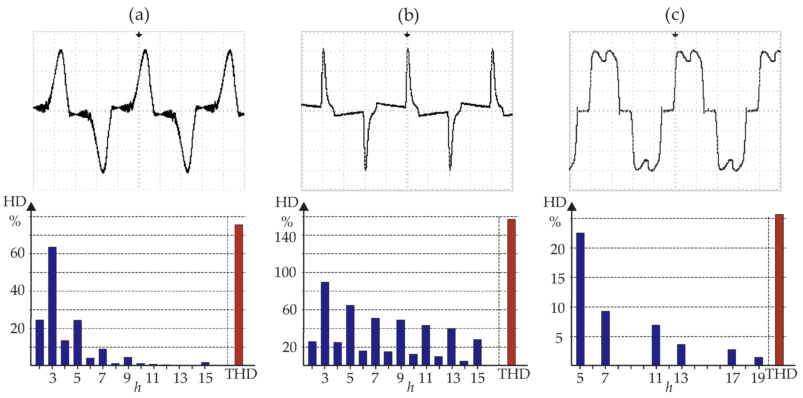
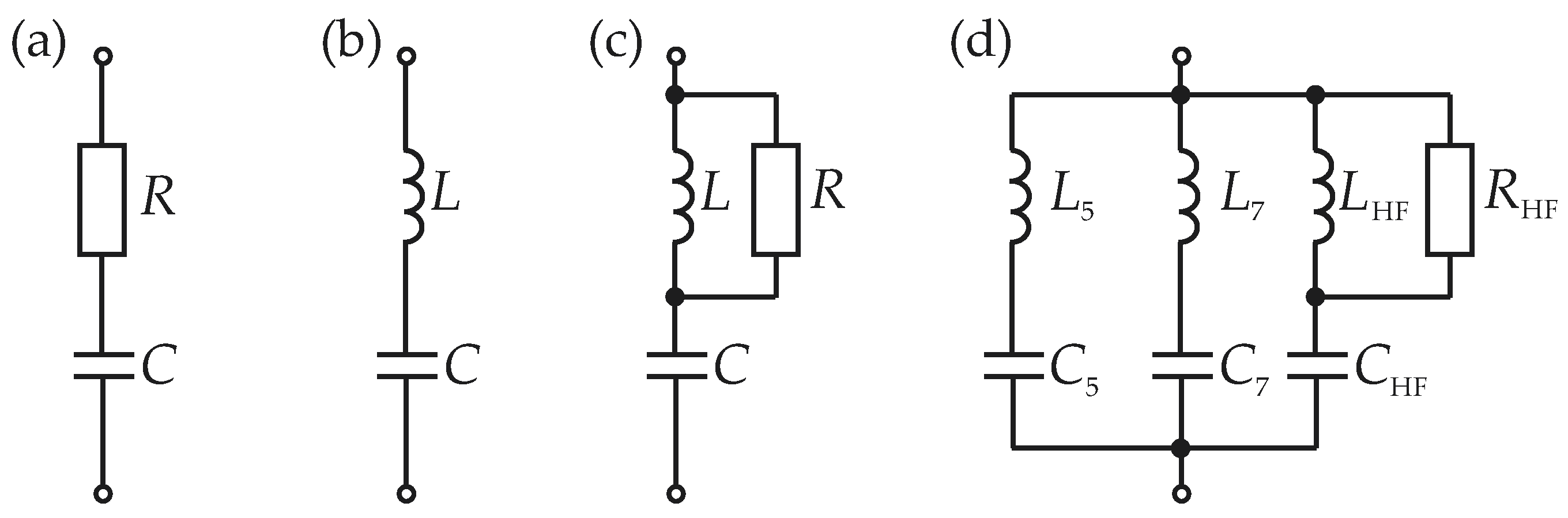
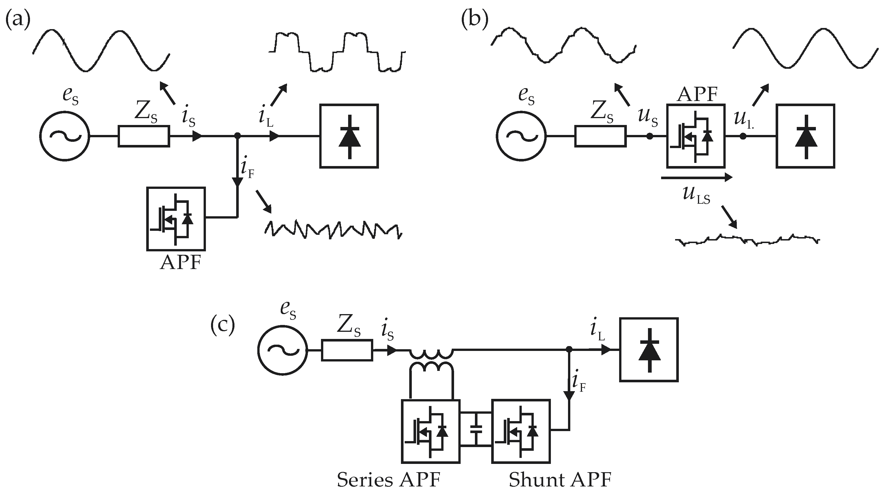
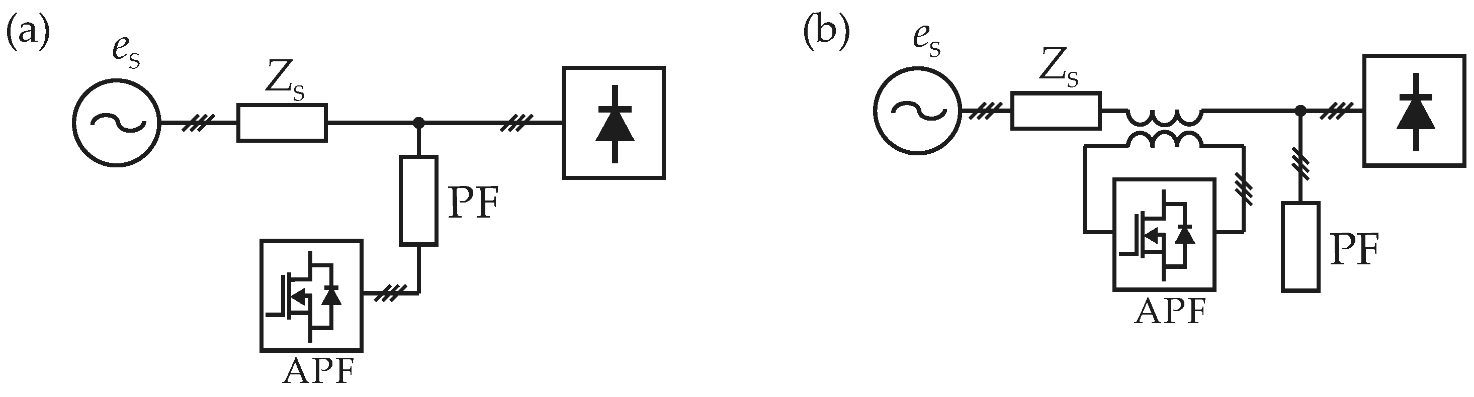
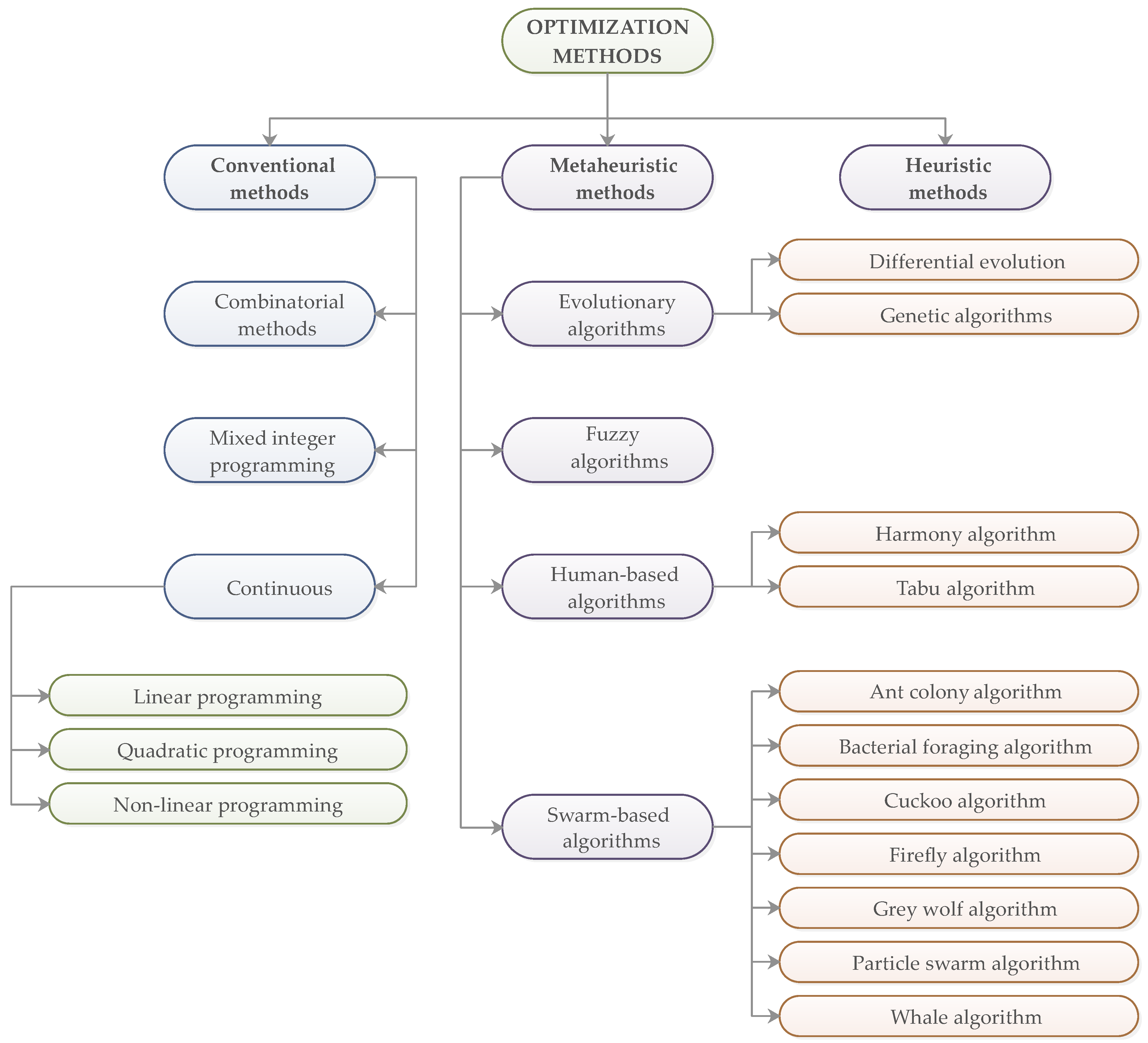
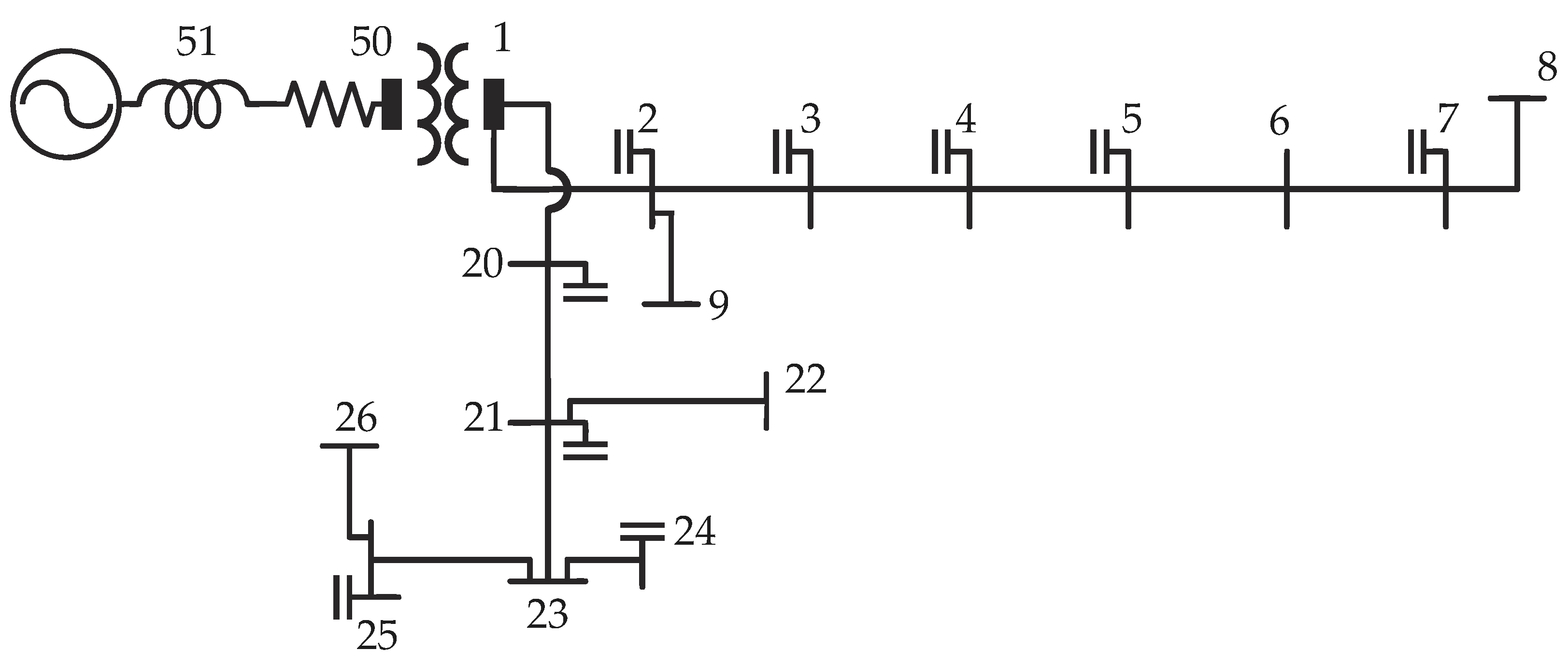
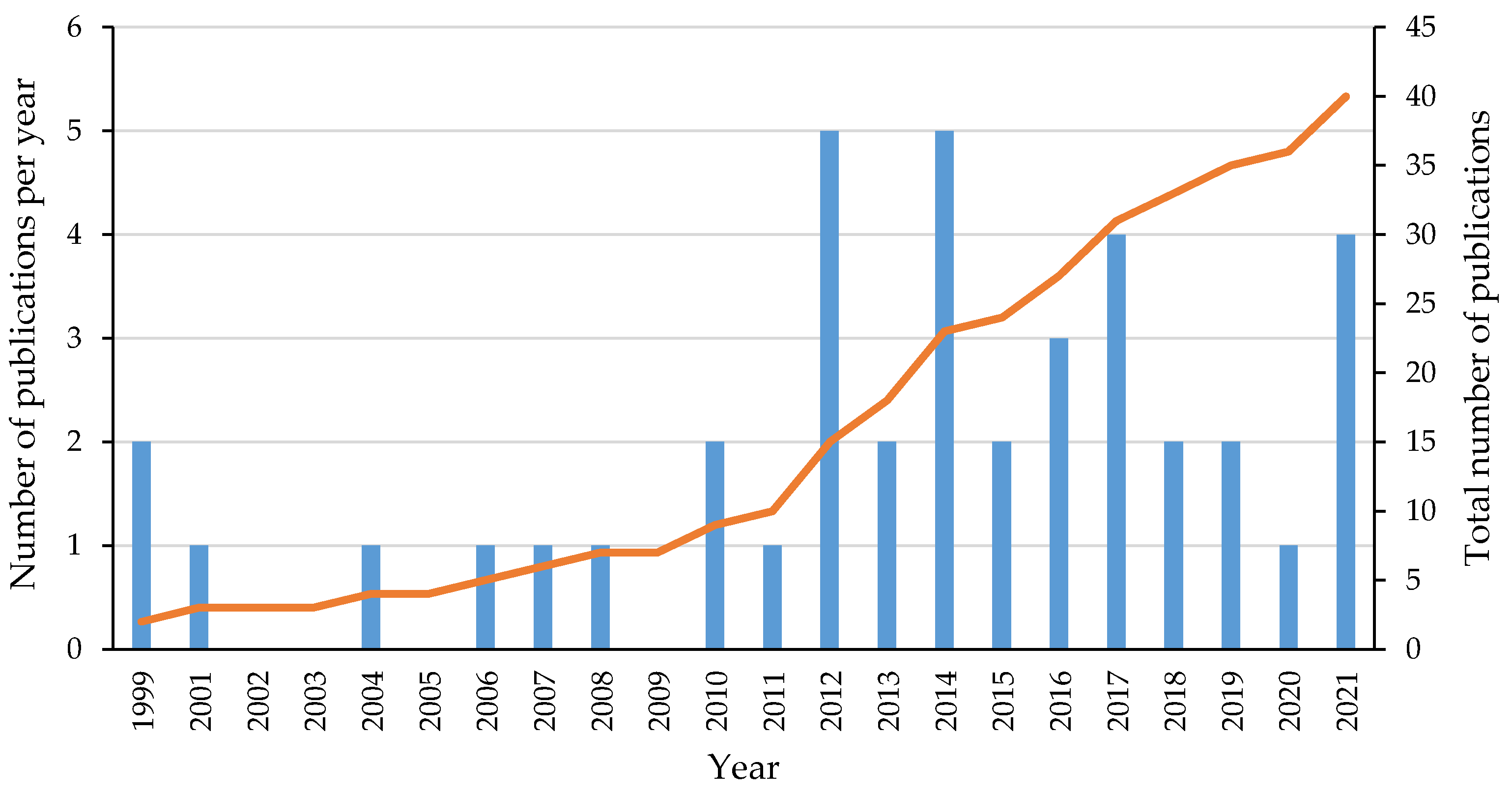
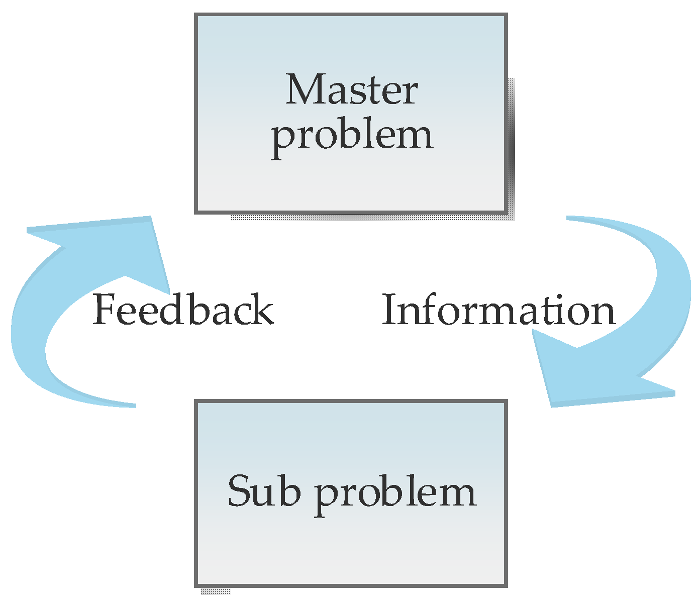
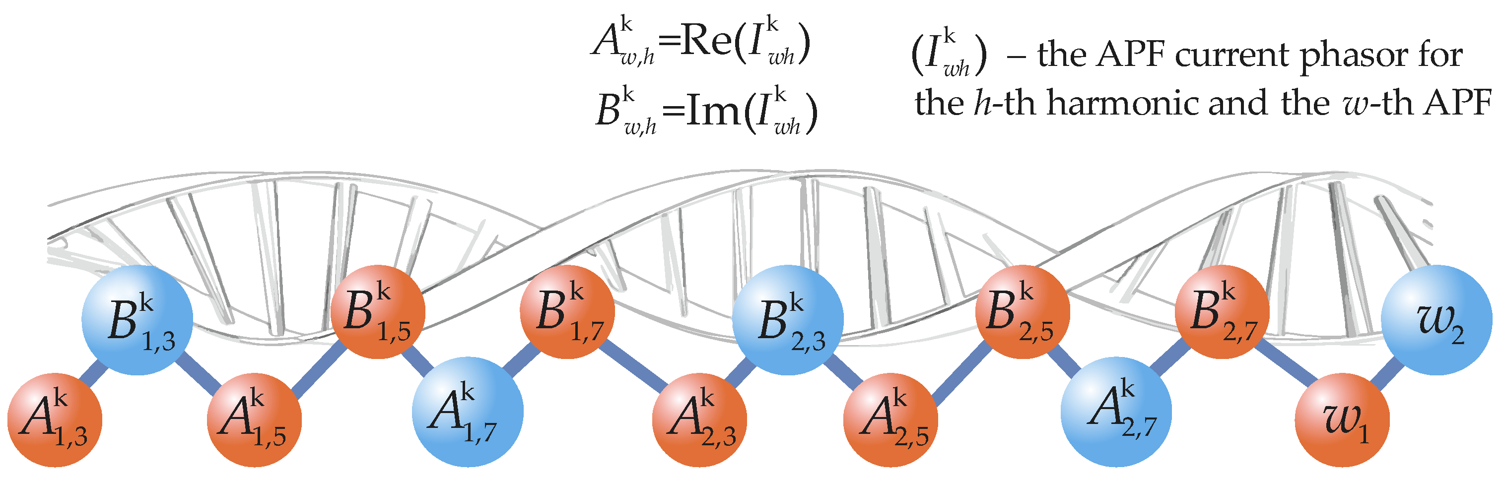
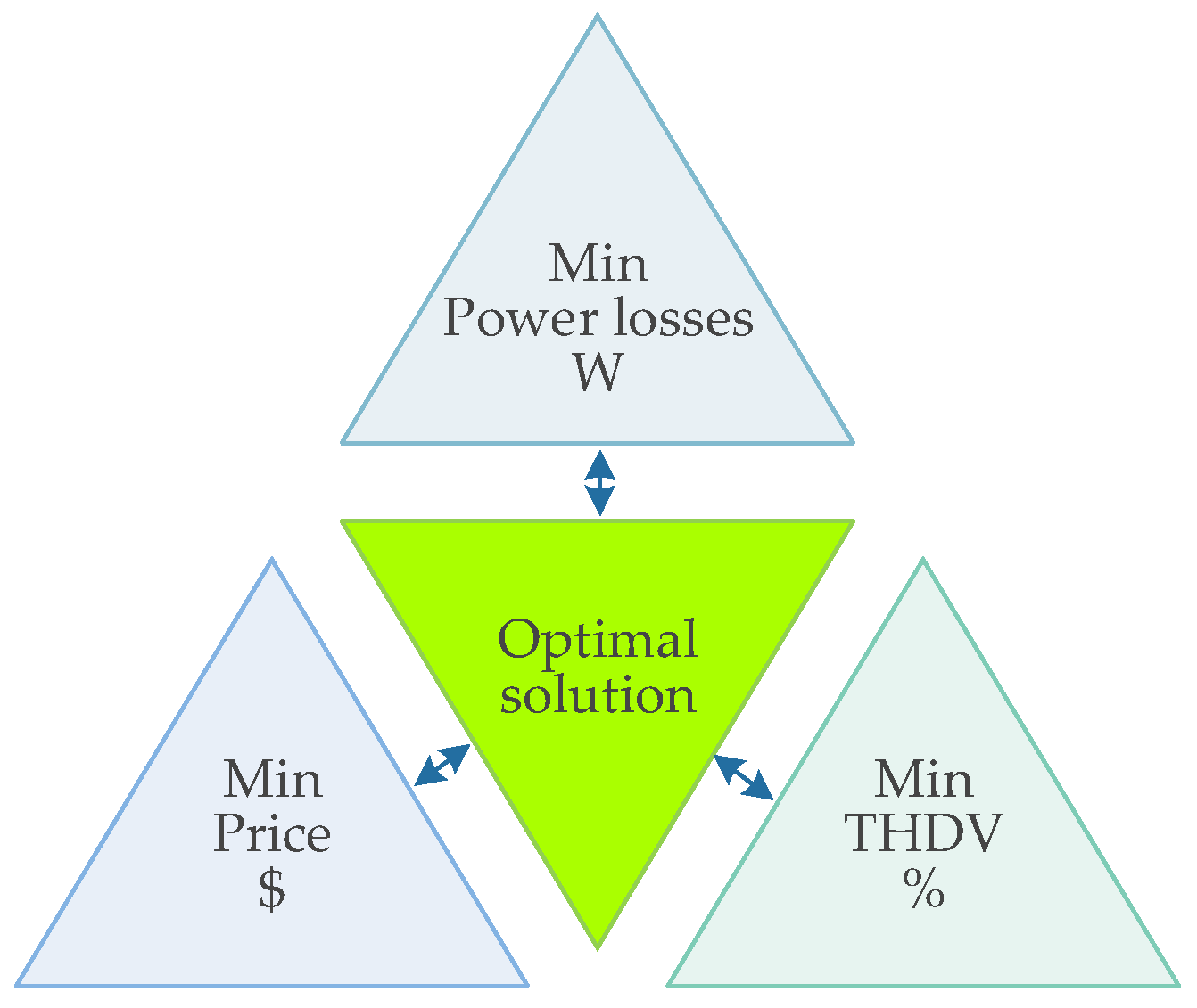
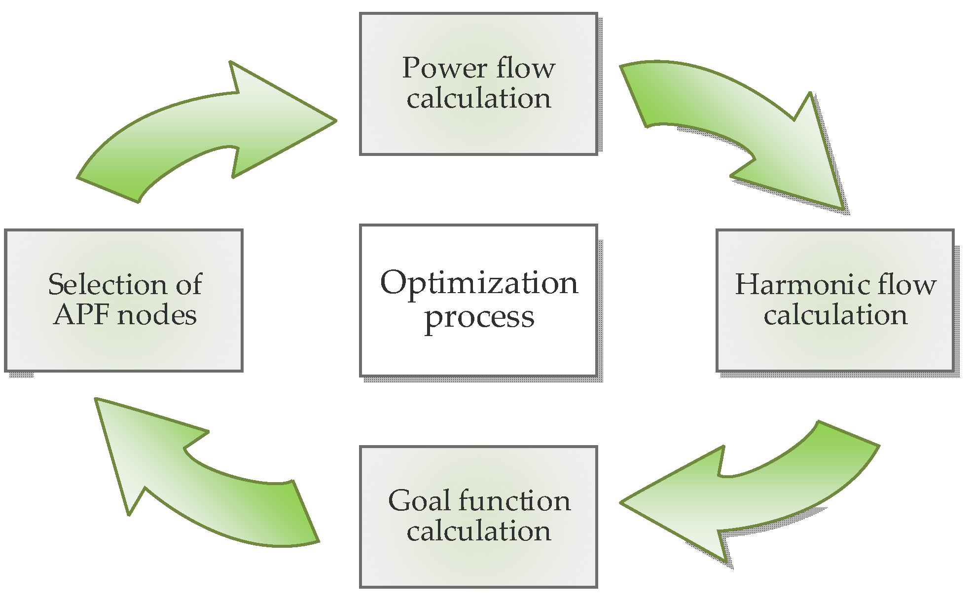
Table 1.
Active power filter functions.
| Function | Shunt APF | Series APF | UPQC |
|---|---|---|---|
| Current harmonic reduction | • | ○ | • |
| Voltage harmonic reduction | ○ | • | • |
| Reactive power compensation | • | • | |
| Voltage flicker reduction | ○ | • | • |
| Removing voltage swells, sags | ○ | • | • |
| Improving load balancing | • | • | |
| Neutral current compensation | • | • |
•−directly, ○−indirectly.
Table 2.
Goal functions and constraints (S, single goal function; M, multi-objective).
| Method | Goal functions | Constraints | Type | References | |
|---|---|---|---|---|---|
| Classical | combinatorial | 9 | A, D | S | [125] |
| 3a | A | S | [125] | ||
| 5e | E | S | [126] | ||
| 1a | E | S | [127] | ||
| 1g | E | S | [128] | ||
| 1g, 4a | C, E | M | [124] | ||
| iterative | 1a, 3a | A, D, E | M | [129] | |
| 4a, 5a | M | [130] | |||
| 3a | S | [131] | |||
| 3a | A, E | S | [131] | ||
| 1a, 1b, 1c, 1d, 1g, 5e | A, B, D, E | S | [132] | ||
| 1a, 5f | A, E | S | [133] | ||
| 1g, 4b, 5b, 6, 8b | D, E | M | [134,135] | ||
| Metaheuristic | Evolutionary algorithms | 1a | C, D, E | S | [136] |
| 3a | A | S | [111] | ||
| 1a | A, C, D, E | S | [111] | ||
| 5c | S | [137] | |||
| 1a, 5d | M | [112] | |||
| 1a, 4a, 5d, e8, ab | M | [113] | |||
| 1g | A, B, D, E | S | [128] | ||
| 1g | A, E | S | [138] | ||
| 1g, 2, 4b | D, E | M | [139] | ||
| 5f | A, D, E | S | [140] | ||
| 1f, 4b | E | M | [123] | ||
| fuzzy | 1a | A, C, D, E | S | [114] | |
| 1e, 4b, 5f, 5g | A, C, D, E, F, G | M | [141] | ||
| 1e + 1c | A, C, D, E | S | [131] | ||
| human | 1e | A, D, E | S | [142] | |
| 1a, 4a, 5f, 7 | A, C, D, E | M | [115] | ||
| swarm-PSO | 1a, 4a, 5f, 7 | A, D, E | M | [116] | |
| 1e | C, D, E | S | [143] | ||
| 4a, 4c | D, E | M | [144] | ||
| 1a, 4a, 5f, 7 | A, E | M | [145] | ||
| 1a, 5f | A, D, E | M | [146] | ||
| 1a, 5f, 9 | E | M | [147] | ||
| 1e | A, D, E | S | [122] | ||
| swarm-other | 1a, 5d | M | [117] | ||
| 4a | D, E | S | [148] | ||
| 1f, 3b, 5f | A, E | M | [149] | ||
| 1a | A, D, E | S | [118,119,120] | ||
| 1e | A, D, E | S | [150] | ||
Table 3.
Used test system sizes.
| Test System Size | References |
|---|---|
| 4-bus | [112,113,117] |
| 5-bus | [114] |
| 6-bus | [120] |
| 7-bus, 9-bus | [125] |
| 11-bus | [137] |
| 13-bus | [148] |
| 15-bus | [146] |
| 16-bus | [149] |
| 17-bus | [126,127,128,132,133,134,135,152] |
| 18-bus | [111,114,115,116,121,129,131,141,143,147] |
| 19-bus | [145] |
| 20-bus | [124,140,142] |
| 23-bus | [136] |
| 25-bus | [139] |
| 30-bus | [116] |
| 33-bus | [118,119,120,121,122] |
| 37-bus | [144] |
| 69-bus | [122,123,150] |
| 95-bus | [123] |
| 119-bus | [123] |
| 123-bus | [139] |
| 445-bus | [138] |
Publisher’s Note: MDPI stays neutral with regard to jurisdictional claims in published maps and institutional affiliations. |
© 2022 by the authors. Licensee MDPI, Basel, Switzerland. This article is an open access article distributed under the terms and conditions of the Creative Commons Attribution (CC BY) license (https://creativecommons.org/licenses/by/4.0/).
Share and Cite
MDPI and ACS Style
Buła, D.; Grabowski, D.; Maciążek, M. A Review on Optimization of Active Power Filter Placement and Sizing Methods. Energies 2022, 15, 1175. https://doi.org/10.3390/en15031175
AMA Style
Buła D, Grabowski D, Maciążek M. A Review on Optimization of Active Power Filter Placement and Sizing Methods. Energies. 2022; 15(3):1175. https://doi.org/10.3390/en15031175
Chicago/Turabian StyleBuła, Dawid, Dariusz Grabowski, and Marcin Maciążek. 2022. "A Review on Optimization of Active Power Filter Placement and Sizing Methods" Energies 15, no. 3: 1175. https://doi.org/10.3390/en15031175
Note that from the first issue of 2016, this journal uses article numbers instead of page numbers. See further details here.