
Self-Triggered Model Predictive Control of AC Microgrids with Physical and Communication State Constraints
by
 ,
,
Xiaogang Dong
1, 
Jinqiang Gan
1,*,
Hao Wu
2,
Changchang Deng
1,
Sisheng Liu
1 and
Chaolong Song
1 1
School of Mechanical Engineering and Electronic Information, China University of Geosciences, Wuhan 430074, China
2
School of Chemistry and Chemical Engineering, Huazhong University of Science and Technology, Wuhan 430074, China
*
Author to whom correspondence should be addressed.
Energies 2022, 15(3), 1170; https://doi.org/10.3390/en15031170
Submission received: 24 December 2021
/
Revised: 23 January 2022
/
Accepted: 30 January 2022
/
Published: 5 February 2022
(This article belongs to the Special Issue Challenges and Research Trends of Distributed Control and Optimization)
Abstract
:In this paper, we investigate the secondary control problems of AC microgrids with physical states (i.e., voltage, frequency and power, etc.) constrained in the process of actual control, namely, under the condition of state constraint. On the basis of the primary control (i.e., droop control), the control signals generated by distributed secondary control algorithm are used to solve the problems of voltage and frequency recovery and power allocation for each distributed generators (DGs). Therefore, the model predictive control (MPC) with the mechanism of rolling optimization is adopted in the second control layer to achieve the above control objectives and solve the physical state constraint problem at the same time. Meanwhile, in order to reduce the communication cost, we designed the self-triggered control based on the prediction mechanism of MPC. In addition, the proposed algorithm of self-triggered MPC does not need sampling and detection at any time, thus avoiding the design of observer and reducing the control complexity. In addition, the Zeno behavior is excluded through detailed analysis. Furthermore, the stability of the algorithm is verified by theoretical derivation of Lyapunov. Finally, the effectiveness of the algorithm is proved by simulation.
1. Introduction
The microgrid, as the newly emerging and rapidly developing smart grid, has good integration capability, namely, it can integrate the energy generated by various small distributed energy systems and power generation equipment [1,2,3]. Therefore, it is often used in parallel power grids and isolated power grids [4,5]. In general, such a problem needs to be solved in the operation of AC microgrids, namely, adjusting the voltage and frequency of all DGs to be the same as that of the total grid [6,7,8,9]. The earliest method to deal with this problem is droop control, but due to the droop coefficient, there is always a certain deviation in the process of voltage and frequency regulation [10,11]. Therefore, on this basis, centralized [12], decentralized [13] and distributed [14] secondary control ideas are put forward, through the secondary control signal to adjust the voltage and frequency deviation. The idea of distributed secondary control mainly comes from distributed multi-agent system [15,16,17]. Due to the voltage and frequency deviation accurately being restored to the same as the total grid by the secondary control, it has strong practical application value for the realization of a high quality AC microgrid without deviation.
Furthermore, in order to reduce the operating cost and improve the working efficiency of the microgrid, the active power of each DG is usually allocated optimally in a certain proportion [18,19]. Usually the idea of hierarchical control is used to achieve this control goal, namely, on the basis of secondary control, an additional controller is added to optimize the distribution of active power [20,21,22]. However, due to the large number of control layers, hierarchical control is usually easy to lead to long control time, slow system operation and other problems. Therefore, in [23], an effective scheme is proposed to further control the optimal power distribution problem by using secondary control so as to save running time. However, due to the need for additional control of incremental costs, redundant control is often generated, which increases the computational burden of the system. Hence, it is of great significance to design a control system which can not only recover voltage and frequency deviation but also realize optimal active power allocation and reduce the calculation burden and communication cost.
On the other hand, most of the states in the operation of microgrids have practical physical significance, such as voltage, frequency active power and so on. Therefore, these physical states are usually inevitably constrained to a certain extent [24], whereas the existing secondary control and hierarchical control are basically lacking effective means to solve the constraint problem. In comparison, the model predictive control (MPC) is an effective solution to the state constraint problem [25,26,27,28]. Thanks to its unique rolling optimization mechanism, the MPC is widely used to deal with control problems with strong constraints. The MPC prediction mechanism and the optimization mechanism are usually used to improve the control performance of AC microgrid [29,30], namely, to solve the problems of voltage and frequency recovery and optimal active power allocation in traditional secondary control. However, in the process of realizing the control goal of the AC microgrid, only a few studies consider the physical state constraints [31]. Therefore, it is of great reference significance to propose more effective MPC control algorithms to solve the problem of physical state constraints in AC microgrids.
Moreover, due to the complex prediction mechanism of the MPC, it usually increases the computational burden and the communication burden of the system. The triggered and self-triggered events are traditional effective methods to reduce communication costs and computational burden [32]. Compared with the event triggered model, the self-triggered model does not need to detect the system state at any time, (i.e., without the observer), thus reducing the computational complexity [33,34]. In addition, the self-triggered model can obtain the exact time of the next triggered moment, so it is widely used in the control of reducing the communication cost and calculation burden of the system [35]. As far as we know, there is little research on using MPC to solve the constraint problem of AC microgrids and reduce the communication cost, which are still in the blank stage. Therefore, it is of great practical value to design a control system that can not only realize the voltage and frequency recovery and optimal active power allocation of AC microgrids but also meet the constraints of the physical state and the communication state.
Based on the above research background, we propose the self-triggered model predictive control based on secondary control, which is used to solve the problems of voltage and frequency recovery and optimal active power allocation for an AC microgrid with physical and communication state constraints. In addition, the Zeno behavior is excluded through systematic theoretical analysis. Finally, the effectiveness of the proposed algorithm is verified by Lyapunov stability theory and simulation experiments. The main contributions are three-fold:
- (1)
- Due to the limitations of power generation equipment and other hardware facilities (such as transformers, inverters, communication equipment, etc.), the physical state (voltage, frequency, power, etc.) of an AC microgrid is inevitably constrained. Compared with [1,2,3], the proposed algorithm based on the rolling optimization mechanism of MPC can also better solve the problem of physical state constraints on the basis of realizing the above control objectives.
- (2)
- In the problem of optimal active power allocation, the hierarchical control (the third control) is usually used [20,21,22]. However, due to the increase in control times, the control time side will be long, which is not conducive to the rapid recovery and stability of the system. By contrast, the proposed algorithm can achieve the control objectives of both voltage and frequency recovery and optimal active power allocation in the secondary control to avoid the above shortcomings.
- (3)
- In an AC microgrid with a complex communication network, the problem of the excessive communication cost has to be considered. Compared with [28,29,30], we designed the scheme of self-triggered control for the prediction mechanism of the MPC, which avoids the disadvantage of needing to sample at any time for the traditional event triggered and does not require additional design of the observer. Meanwhile, the scheme not only reduces the communication cost and computation burden but also does not have Zeno behavior.
The organization of the remaining parts is as follows. The preliminaries are given in Section 2. The self-triggered model predictive control in AC microgrids is presented in Section 3. Section 4 presents the results. The simulations are shown in Section 5, and the conclusions are drawn in Section 6.
Notations: denotes the real number field. represents the n-dimensional Euclidean space. represents the n-dimensional row vector with its all elements being 1. denotes the Euclidean norm. for all and , where Q is positive definite or semi-positive definite.
2. Preliminaries
In this section, we introduce the structure of traditional secondary control used to solve the control objectives of an AC microgrid. Meanwhile, the various control objectives of the AC microgrid are explained in detail.
2.1. Communication of AC Microgrids
In an AC microgrid, it needs to obtain useful information through the communication exchange for each independent distributed generator (DG), so as to achieve the overall control goal cooperatively. In order to reduce the communication cost, we define a hierarchical directed graph (Figure 1b) to simplify the general topology graph (Figure 1a) as follows. Firstly, the general topology graph is divided into the following three layers according to the number of adjacent DG. Secondly, the first layer is used as the leader to track the control target directly, as well the subsequent layers track the previous layer in turn. The specific tracking target for each layer meets the following conditions:
where represents the total tracking target, namely, the reference value. represents the state of the i-th DG. represents the adjacency matrix, i.e., the set of all adjacent to .
Remark 1.
These hierarchical directed graphs can simplify both directed graphs and undirected graphs. Just make sure there is at least one communication between each layer.
2.2. Secondary Control of AC Microgrids
We consider the AC microgrid composed of i DG, . The inverter-based secondary control framework composed of various electrical components and control circuits is shown in Figure 2. Please refer to [36] for the specific structure of various electrical components. The control principle contained the two parts. Firstly, the voltage and frequency are preliminarily adjusted by the droop control (namely, the primary control) in the power controller. Secondly, the voltage and frequency are recovered by the secondary control. Finally, the obtained voltage and frequency are input into the inverter-based DG control framework to realize the control of the total current and voltage of the AC microgrid.
The traditional droop control in the power controller meets the following conditions [37]:
where and represent the angular frequency and its nominal value, respectively. and are the d-axis and q-axis voltages, respectively. represent the nominal value of . and are the active and reactive power, respectively, and and are the droop coefficients. represents the terminal voltage, and can be obtained from (2). Therefore, is replaced by in the latter part in the paper.
The internal loop of the inverter-based DG control framework meets the following conditions [37]:
where the state vector ; a known disturbance ; represents the relative angle of in the common reference frame; the direct component and the quadratic component are regarded as the auxiliary variable of the voltage controller; the direct component and the quadratic component denote the auxiliary variable of the current controller, respectively; and and are the variables associated with the LC filter and output connector. Refer to [36] for detailed expressions of and .
Based on the above research content, in order to achieve the goals of frequency and voltage recovery and optimal active power allocation, taking the derivative of (2), the following secondary control is designed:
where and represent the secondary control signals of the frequency, voltage and active power in turn. represents the cutoff frequency of low-pass filter. According to (4), and can be obtained as follows:
2.3. Theory Basics
The system is considered as follows:
where and represent the state and control input of i-th DG, and A and B are known stabilized matrices.
According to the tracking target (1) and the state Equation (6), the problem of the following rolling optimization is constructed:
:
where represents the prediction horizontal, R is a semi-definite matrix, and Q and P represent positive definite matrices. in brackets denotes the state at time , predicted at time k, . Equation (7b) is the prediction model, , and are the compact set, representing state and control signal constraints. Equation (7d) stands for the terminal constraint. are the tracking targets. The partial derivative of the above cost function is taken to obtain the optimal control sequence . Then, the first item of the sequence of optimal control is used as the control input :
By putting the control input into the system (6), the tracking target can be achieved.
Generally, define as the self-triggered instants of and , as the sequence of self-triggered instants; namely, at time , the rolling optimization mechanism of the MPC is updated to obtain the optimal control sequence, as well to obtain the next self-triggered instants according to the specific self-triggered conditions [1], namely, , . In other words, the controller of each is only updated at the self-triggered instants , as well transmits the newly acquired information to its neighbor . In the time interval from to , the controller stops updating but uses the control input obtained at the previous trigger time, so as to reduce the communication cost and computation burden.
Assumption 1.
The topology graph under consideration has a directed spanning tree, and the root can be regarded as the leader of the layered directed graph.
Assumption 2.
There exist corresponding Lipschitz constants and for Lipschitz continuous functions and . Simultaneously, there is the function that makes true.
Lemma 1
([38]). The discretized equation of the prediction model is rewritten as follows based on the forward Euler method: , where , , T represents the sampling time.
Lemma 2
Refer to stability analysis for a detailed proof of Lemma 2.
3. Self-Triggered Model Predictive Control in AC Microgrids
In this part, we design a self-triggered model predictive control to solve the secondary control problem in AC microgrid according to the specific prediction mechanism of the MPC. In addition, the voltage and frequency recovery targets of AC microgrid are achieved, simultaneously, the optimal active power allocation is also accomplished.
3.1. Self-Triggered Model Predictive Control
In general, model predictive control (MPC) only takes the first term as the effective control input and abandons the remaining predictive control input, after solving the rolling optimization problem to obtain the optimal control sequence. Although this will achieve a better control effect, the abandonment of a large number for predicted values will cause a large degree of calculation waste, as well as greatly increasing the calculation burden. Therefore, we design a self-triggered control scheme based on the prediction mechanism of the MPC, which can effectively choose the predicted control input in optimal control sequence. Meanwhile, it can greatly reduce the communication cost and calculation burden on the premise of ensuring system stability.
Definition 1.
If the Assumptions 1 and 2 are guaranteed and system (6) has a solution at time , there exists and satisfying:
Therefore, the next triggered time can be selected according to the following conditions:
where and are given in Lemma 2, and is represented in (15).
First of all, the following feasible control inputs are constructed at time :
where represents the optimal control input obtained by solving the optimization problem at time , , which represents the feasible control input at terminal time . Put it into system (6) to obtain the corresponding feasible state and the optimal state of .
Generally, in order to ensure the stability of the system using the MPC, it only needs to satisfy that the value of the cost function at the next triggered instant is less than that at the previous triggered instant, namely, .
Through substituting the feasible input (12) at time into the cost function (7a), the following feasible value of the cost function at time can be obtained:
Based on the fact that the value of the feasible cost function must be greater than or equal to the value of the optimal cost function, namely, , therefore, (13) can be rewritten as follows:
where , , .
Therefore, the stability of the system can be guaranteed, namely: if the following conditions are met:
If the condition (15) above is violated, i.e., the self-triggered condition is triggered, the control state of the system will be updated. However, in order to calculate the next triggered time more easily, we reconstructed the condition (15) as follows:
where is chosen differently for each .
Remark 2.
Compared with the self-triggered condition (15), the triggered requirement of self-triggered condition (16) becomes higher due to and being discarded. This causes the cost function of the system to increase briefly during the phase in which condition (15) is triggered but condition (16) is not. However, since the time of the increment is very short, and the normal number is introduced into condition (16) to reduce the triggered condition, this problem will not affect the consistency convergence of tracking targets and the stability of the system.
3.2. Voltage and Frequency Recovery with Physical State Constraints
In general, in AC microgrids, the voltage and frequency cannot be completely adjusted to the nominal value only through the traditional droop control, so it is necessary to use a secondary control to achieve voltage and frequency recovery. However, the voltage and frequency are physical quantities, which will inevitably be limited by various power generation equipment and other hardware facilities. Therefore, we define such physical state constraints as follows.
Definition 2.
In the whole secondary control process, there exists a compact set such that the state of the i-th DG, where , , is the initial state.
In order to achieve voltage and frequency recovery with state constraints, according to the theory of model predictive control and Lemma 1, we rewrite secondary control (4) into the following:
where , and represent the status and the control input of the voltage and frequency, respectively.
Taking (17) as the prediction model and combining it with the self-triggered control, the following optimization problem is constructed:
Problem 1.
By solving the above optimization Problem 1, the predictive control sequence is obtained. Moreover, according to the self-triggered condition (11), the useful control input is selected as follows:
Afterwards, the useful control input is put into the prediction model (17) to obtain the state of voltage and frequency, while the control input of voltage and frequency is put into (5) to obtain and , which are fed back to the droop control to form a closed-loop system. Finally, the voltage and frequency recovery is achieved.
3.3. Optimal Active Power Allocation Based on Secondary Control
Usually, after the secondary control adjustment of the frequency, the active power also needs to meet the corresponding allocation conditions, namely:
In order to avoid designing additional controllers, according to the tracking target (1), the control target (20) is rewritten as follows:
where , denotes the total tracking target. represents the power of the i-th DG. represents the adjacency matrix, i.e., the set of all adjacent to .
Therefore, we can still use the self-triggered MPC for the secondary regulation of active power. Firstly, in (4) is discretized according to Lemma 1, namely:
where , and represent the status and the control input of power, respectively.
Similarly, taking (22) as the prediction model and combining it with the self-triggered control, the following optimization problems can be obtained:
Problem 2.
Similarly, the optimal control sequence is obtained by solving the optimization Problem 2. Therefore, select the useful control input as follows:
Put the useful control inputs into (22) to obtain the active power. Finally, achieve the goal of the active power allocation through repeated secondary control and adjustment using the self-triggered MPC.
4. Results
In this part, we will analyze the stability of the proposed self-triggered MPC and deduce Lemma 2 in detail. In addition, we also exclude the Zeno behavior through theoretical analysis.
4.1. Stability Analysis
Generally, the stability analysis of model’s predictive control is carried out by Lyaplov theory, namely, let the cost function decrease with time; in other words, satisfy . According to the theoretical analysis of (13)–(16), the system stability can be guaranteed if Lemma 2 is established.
Proof.
The corresponding cost functions and can be obtained by substituting different initial values and into the model predictive control system. Then, the cost functions are solved to obtain the predictive control inputs and , as well the corresponding prediction state and , . Combined with the definition of feasible input in (12), the following can be obtained: , , Therefore, it can be further obtained as follows:
Then, by substituting the actual control and optimal control at time into the prediction model (18b), the actual state and optimal state at time can be obtained:
Therefore, according to (26) and the Gronwall–Bellman inequality, can be obtained.
Due to the Lemma 2 being proved, the systems are stable. □
4.2. Elimination of Zeno Behavior
The so-called Zeno behavior usually refers to the phenomenon that the system cannot run normally because the triggered interval is too small for the hardware facilities, for example, the controller cannot meet the high frequency sampling. Therefore, if two consecutive triggered intervals are guaranteed to have lower bounds, the Zeno behavior can be excluded, namely:
where is a positive constant.
Since the proposed self-triggered MPC is based on discrete systems, the triggered interval will take an integer multiple of the sampling period T, obviously the condition (28) can be guaranteed. Therefore, the self-triggered MPC proposed in this paper does not have Zeno behavior.
5. Simulations
In this section, in order to verify the feasibility and effectiveness of the proposed self-triggered MPC algorithm applied to the AC microgrid, the simulation experiments are given from the following three aspects: (1) voltage and frequency recovery; (2) optimal active power allocation; and (3) the triggering time of the the self-triggered MPC.
The parameters of the AC microgrid used in the following simulation experiments are shown in Table 1; simultaneously, the communication topology diagram adopts the directed graph in Figure 1b.
Remark 3.
This paper studies the AC microgrid system with a layered graph composed of multiple DG (similar to multi-agent system). Therefore, for the convenience of the experiment, only six DGs are selected in this paper, but in fact, the algorithm can achieve the same effect no matter how many DGs are given in the simulation experiment, as long as it is an AC microgrid system that meets the conditions of the hierarchical graph and Assumption 1.
5.1. Voltage and Frequency Recovery
In this part, in order to verify that the proposed algorithm can effectively complete the voltage and frequency recovery of the AC microgrid with physical state constraints, the simulation results of different control input constraints with voltage and power constraints are given. In addition, the parameters of the self-triggered MPC control parameters are selected as shown in Table 2.
In Figure 3, it is obvious that the voltage changes of all DGs satisfy the physical state constraint . A time of 0–2 s indicates that the AC microgrid has been stabilized through droop control, but there is still a certain deviation from the target value. Starting from 2 s, the voltage is restored to the rated value through the secondary control using the self-triggered MPC. By comparing the three subgraphs in Figure 3, it can be found that a larger range of control constraints corresponds to a faster convergence time.
Similarly, in Figure 4, the frequency changes of all DGs also meet the physical state constraint condition . Here, 0–2 s is the droop control of AC microgrid. After 2 s, the self-triggered MPC is used to adjust again, so that the frequency is restored to the rated value. Obviously, when the control requirements are reduced, the convergence time will be faster. In summary, the proposed algorithm can solve the voltage and frequency recovery problems of AC microgrid with physical state constraints well.
5.2. Optimal Active Power Allocation
In this section, in order to verify that the optimal allocation of the active power can be achieved without the additional third control, the same self-triggered MPC algorithm is used for the secondary adjustment of active power. The simulation results are shown in Figure 5.
Obviously, the active power also satisfies the physical state constraint . At 0–2 s, the droop control is adopted. After 2 s, the optimal allocation of active power can be finally achieved by the secondary adjustment using the self-triggered MPC. Furthermore, by comparing the three subgraphs in Figure 5, it can be concluded that as long as the control input range is reasonably selected, the active power distribution goal can be achieved in a very short time. Compared with the traditional hierarchical control (the third control), it has more practical application value.
5.3. Triggering Time of the Self-Triggered MPC
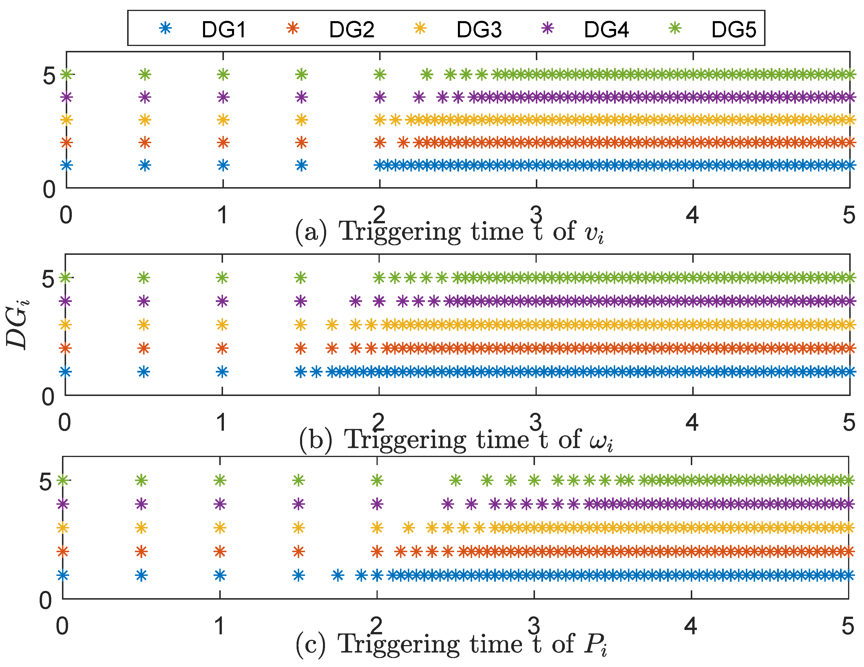
In this part, the simulation results of sampling time of self-triggered MPC algorithm are given in Figure 6. In Figure 6a, within 0 to 2 s, due to being away from tracking the target, the control input requirements are not high. Therefore, all of the 10 predicted values for model predictive control can be adopted. During the period of 2 s to 3 s, the physical state of the voltage is close to the tracking target. Thus, only part of the predicted value is used under the selection of the trigger condition (16). After 3 s, the system has fully achieved the tracking goal, so periodic sampling is maintained. The simulation results in Figure 6b,c are similar. Therefore, compared with the simple MPC, the proposed self-triggered MPC is indeed more beneficial to reduce the communication cost and the calculation burden of the system.
6. Conclusions
In this paper, based on the framework of the inverter-based traditional secondary control in AC microgrid, the proposed self-triggered MPC realizes voltage and frequency recovery with the physical state constraints. Meanwhile, the optimal allocation of active power can be realized by using the proposed algorithm to secondarily adjust the active power without designing the additional third control. Therefore, the complexity of the controller is reduced to a certain extent, and the system convergence can be achieved in a very short time by selecting the control input range reasonably. Moreover, compared with a single MPC, the proposed self-triggered MPC can reduce the communication cost and computation burden of the system. All in all, the proposed self-triggered MPC is more conducive to the practical application and development of an AC microgrid. However, due to space constraints, we will extend this algorithm to more complex AC microgrid systems composed of DG in future research work. As well, we will implement the AC MG in dedicated simulation software with a higher level of details (e.g., harmonics, external grid distortion).
Author Contributions
Conceptualization, J.G. and C.S.; methodology, J.G. and C.D.; software, X.D. and C.D.; validation, X.D.; formal analysis, S.L.; investigation, X.D.; resources, X.D. and J.G.; data curation, X.D. and H.W.; writing—original draft preparation, X.D. and J.G.; writing—review and editing, J.G.; visualization, X.D.; supervision, J.G.; project administration, J.G. and C.S.; funding acquisition, H.W. and J.G. All authors have read and agreed to the published version of the manuscript.
Funding
This work was supported by the National Natural Science Foundation of China ( Nos. 52175035 and 51805494) and National Key Technology R&D Program of China (Grants: 2020YFB1709301, 2020YFB1709304).
Institutional Review Board Statement
Not applicable.
Informed Consent Statement
Not applicable.
Data Availability Statement
Not applicable.
Conflicts of Interest
The authors declare no conflict of interest.
References
- Hu, X.; Liu, Z.W.; Wen, G.; Yu, X.; Liu, C. Voltage control for distribution networks via coordinated regulation of active and reactive power of DGs. IEEE Trans. Smart Grid 2020, 11, 4017–4031. [Google Scholar] [CrossRef]
- Wu, Y.-D.; Ge, M.-F.; Liu, Z.-W.; Zhang, W.-Y.; Wei, W. Distributed CPS-Based secondary control of microgrids with optimal power allocation and limited communication. IEEE Trans. Smart Grid 2022, 13, 82–95. [Google Scholar] [CrossRef]
- Patnaik, B.; Mishra, M.; Bansal, R.C.; Jena, R.K. AC microgrid protection a review: Current and future prospective. Appl. Energy 2020, 271, 115210. [Google Scholar] [CrossRef]
- Lai, J.; Lu, X.; Yu, X.; Monti, A. Stochastic distributed secondary control for ac microgrids via event-triggered communication. IEEE Trans. Smart Grid 2020, 11, 2746–2759. [Google Scholar] [CrossRef]
- Li, Y.; Peng, Y.; Wang, X. Seamless switching power sharing control method in a hybrid DC-AC microgrid by the isolated two-stage converter based on SST. IET Power Electron. 2021, 14, 1384–1396. [Google Scholar] [CrossRef]
- Kaushal, J.; Basak, P. Power quality control based on voltage sag swell, unbalancing, frequency, THD and power factor using artificial neural network in PV integrated AC microgrid. Sustain. Energy Grids Netw. 2020, 23, 100365. [Google Scholar] [CrossRef]
- Behera, M.K.; Saikia, L.C. Combined voltage and frequency control for diverse standalone microgrid networks using flexible IDC with novel FOC: A real-time validation. IETE J. Res. 2021, 1–26. [Google Scholar] [CrossRef]
- Rosini, A.; Minetti, M.; Denegri, G.B.; Invernizzi, M. Reactive power sharing analysis in islanded AC microgrids. In Proceedings of the 2019 IEEE International Conference on Environment and Electrical Engineering and 2019 IEEE Industrial and Commercial Power Systems Europe (EEEIC/I&CPS Europe), Genova, Italy, 11–14 June 2019; pp. 1–6. [Google Scholar] [CrossRef]
- Rosini, A.; Bonfiglio, A.; Invernizzi, M.; Procopio, R.; Serra, P. Power management in islanded hybrid diesel-storage microgrids. In Proceedings of the 2019 IEEE PES Innovative Smart Grid Technologies Europe (ISGT-Europe), Bucharest, Romania, 29 September–2 October 2019; pp. 1–5. [Google Scholar] [CrossRef]
- Yuan, W.; Wang, Y.; Liu, D.; Deng, F.; Chen, Z. Efficiency-prioritized droop control strategy of AC microgrid. IEEE J. Emerg. Sel. Top. Power Electron. 2020, 9, 2936–2950. [Google Scholar] [CrossRef]
- Li, D.; Wu, Z.; Zhao, B.; Zhang, L. An improved droop control for balancing state of charge of battery energy storage systems in AC microgrid. IEEE Access 2020, 8, 71917–71929. [Google Scholar] [CrossRef]
- Xiao, H.; Liu, G.; Huang, J.; Hou, S.; Zhu, L. Parameterized and centralized secondary voltage control for autonomous microgrids. Int. J. Electr. Power Energy Syst. 2022, 135, 107531. [Google Scholar] [CrossRef]
- Liu, B.; Wu, T.; Liu, Z.; Liu, J. A small-AC-signal injection-based decentralized secondary frequency control for droop-controlled islanded microgrids. IEEE Trans. Power Electron. 2020, 35, 11634–11651. [Google Scholar] [CrossRef]
- Chen, Y.; Qi, D.; Dong, H.; Li, C.; Li, Z.; Zhang, J. A FDI attack-resilient distributed secondary control strategy for islanded microgrids. IEEE Trans. Smart Grid 2020, 12, 1929–1938. [Google Scholar] [CrossRef]
- Liu, Z.W.; Hu, X.; Ge, M.F.; Wang, Y.W. Asynchronous impulsive control for consensus of second-order multi-agent networks. Commun. Nonlinear Sci. Numer. Simul. 2019, 79, 104892. [Google Scholar] [CrossRef]
- Ge, M.F.; Liu, Z.W.; Wen, G.; Yu, X.; Huang, T. Hierarchical controller-estimator for coordination of networked Euler-CLagrange systems. IEEE Trans. Cybern. 2019, 50, 2450–2461. [Google Scholar] [CrossRef] [PubMed]
- Ge, M.F.; Guan, Z.H.; Yang, C.; Li, T.; Wang, Y.W. Time-varying formation tracking of multiple manipulators via distributed finite-time control. Neurocomputing 2016, 202, 20–26. [Google Scholar] [CrossRef] [Green Version]
- Wang, Z.; Yi, H.; Zhuo, F.; Wu, J.; Zhu, C. Analysis of parameter influence on transient active power circulation among different generation units in microgrid. IEEE Trans. Ind. Electron. 2020, 68, 248–257. [Google Scholar] [CrossRef]
- Roy, N.B.; Das, D. Optimal allocation of active and reactive power of dispatchable distributed generators in a droop controlled islanded microgrid considering renewable generation and load demand uncertainties. Sustain. Energy Grids Netw. 2021, 27, 100482. [Google Scholar] [CrossRef]
- Lu, X.; Xia, S.; Sun, G.; Hu, J.; Zou, W.; Zhou, Q.; Chan, K.W. Hierarchical distributed control approach for multiple on-site DERs coordinated operation in microgrid. Int. J. Electr. Power Energy Syst. 2021, 129, 106864. [Google Scholar] [CrossRef]
- Wu, X.; Xu, Y.; He, J.; Wang, X.; Vasquez, J.C.; Guerrero, J.M. Pinning-based hierarchical and distributed cooperative control for AC microgrid clusters. IEEE Trans. Power Electron. 2020, 35, 9865–9885. [Google Scholar] [CrossRef]
- Vilaisarn, Y.; Moradzadeh, M.; Abdelaziz, M.; Cros, J. An MILP formulation for the optimum operation of AC microgrids with hierarchical control. Int. J. Electr. Power Energy Syst. 2022, 137, 107674. [Google Scholar] [CrossRef]
- Lian, Z.; Deng, C.; Wen, C.; Guo, F.; Lin, P.; Jiang, W. Distributed event-triggered control for frequency restoration and active power allocation in microgrids with varying communication time delays. IEEE Trans. Ind. Electron. 2020, 68, 8367–8378. [Google Scholar] [CrossRef]
- Dehkordi, N.M.; Nekoukar, V. Robust distributed stochastic secondary control of microgrids with system and communication noises. IET Gener. Transm. Distrib. 2020, 14, 1148–1158. [Google Scholar] [CrossRef]
- Hu, J.; Shan, Y.; Guerrero, J.M.; Ioinovici, A.; Chan, K.W.; Rodriguez, J. Model predictive control of microgrids—An overview. Renew. Sustain. Energy Rev. 2021, 136, 110422. [Google Scholar] [CrossRef]
- Chen, T.; Abdel-Rahim, O.; Peng, F.; Wang, H. An improved finite control set-MPC-based power sharing control strategy for islanded AC microgrids. IEEE Access 2020, 8, 52676–52686. [Google Scholar] [CrossRef]
- Batiyah, S.; Sharma, R.; Abdelwahed, S.; Zohrabi, N. An MPC-based power management of standalone DC microgrid with energy storage. Int. J. Electr. Power Energy Syst. 2020, 120, 105949. [Google Scholar] [CrossRef]
- Zheng, C.; Dragičević, T.; Blaabjerg, F. Model predictive control-based virtual inertia emulator for an islanded alternating current microgrid. IEEE Trans. Ind. Electron. 2020, 68, 7167–7177. [Google Scholar] [CrossRef]
- Blanco, A.; Labella, D.; Mestriner, D.; Rosini, A. Model predictive control for primary regulation of islanded microgrids. In Proceedings of the 2018 IEEE International Conference on Environment and Electrical Engineering and 2018 IEEE Industrial and Commercial Power Systems Europe (EEEIC/I&CPS Europe), Palermo, Italy, 12–15 June 2018; pp. 1–6. [Google Scholar] [CrossRef]
- Rosini, A.; Mestriner, D.; Labella, A.; Bonfiglio, A.; Procopio, R. A decentralized approach for frequency and voltage regulation in islanded PV-Storage microgrids. Electr. Power Syst. Res. 2021, 193, 106974. [Google Scholar] [CrossRef]
- Gan, L.K.; Zhang, P.; Lee, J.; Osborne, M.A.; Howey, D.A. Data-driven energy management system with Gaussian process forecasting and MPC for interconnected microgrids. IEEE Trans. Sustain. Energy 2020, 12, 695–704. [Google Scholar] [CrossRef]
- Xu, J.Z.; Ge, M.F.; Liu, Z.W.; Zhang, W.Y.; Wei, W. Force-reflecting hierarchical approach for human-aided teleoperation of NRS with event-triggered local communication. IEEE Trans. Ind. Electron. 2022, 69, 2843–2854. [Google Scholar] [CrossRef]
- Wang, L.; Ge, M.F.; Zeng, Z.; Hu, J. Finite-time robust consensus of nonlinear disturbed multiagent systems via two-layer event-triggered control. Inf. Sci. 2018, 466, 270–283. [Google Scholar] [CrossRef]
- Wan, X.; Tian, Y.; Wu, J.; Ding, X.; Tu, H. Distributed event-triggered secondary recovery control for islanded microgrids. Electronics 2021, 10, 1749. [Google Scholar] [CrossRef]
- Xu, G.; Ma, L. Resilient self-triggered control for voltage restoration and reactive power sharing in islanded microgrids under Denial-of-Service attacks. Appl. Sci. 2020, 10, 3780. [Google Scholar] [CrossRef]
- Pogaku, N.; Prodanovic, M.; Green, T.C. Modeling, analysis and testing of autonomous operation of an inverter-based microgrid. IEEE Trans. Power Electron. 2007, 22, 613–625. [Google Scholar] [CrossRef] [Green Version]
- Bidram, A.; Davoudi, A.; Lewis, F.L.; Qu, Z. Secondary control of microgrids based on distributed cooperative control of multi-agent systems. IET Gener. Transm. Distrib. 2013, 7, 822–831. [Google Scholar] [CrossRef] [Green Version]
- Milošević, M. Convergence and almost sure polynomial stability of the backward and forward-backward Euler methods for highly nonlinear pantograph stochastic differential equations. Math. Comput. Simul. 2018, 150, 25–48. [Google Scholar] [CrossRef]
- Duan, J.; Zhang, H.; Wang, Y.; Han, J. Output consensus of heterogeneous linear MASs by self-triggered MPC scheme. Neurocomputing 2018, 315, 476–485. [Google Scholar] [CrossRef]
Figure 1.
The communication topology of an AC microgrid: (a) the general communication topology; (b) the hierarchical topology after simplification.
Figure 1.
The communication topology of an AC microgrid: (a) the general communication topology; (b) the hierarchical topology after simplification.
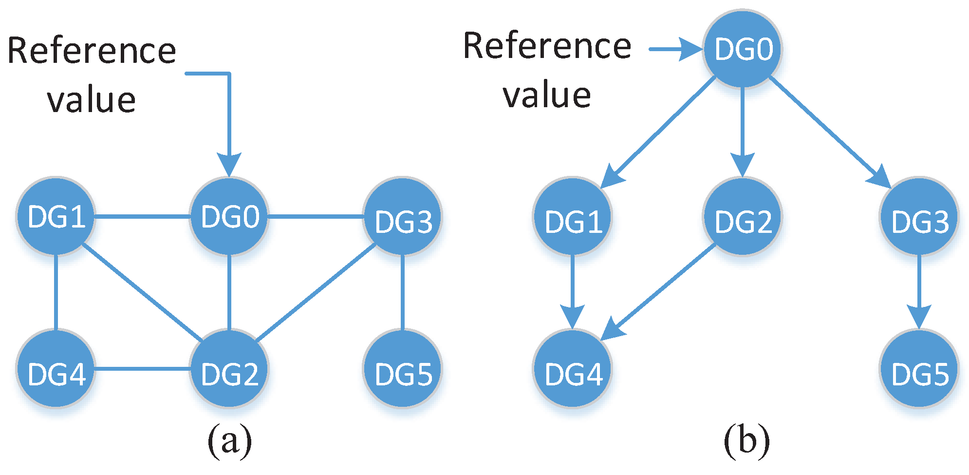
Figure 2.
The framework of the inverter-based secondary control using the self-triggered MPC.
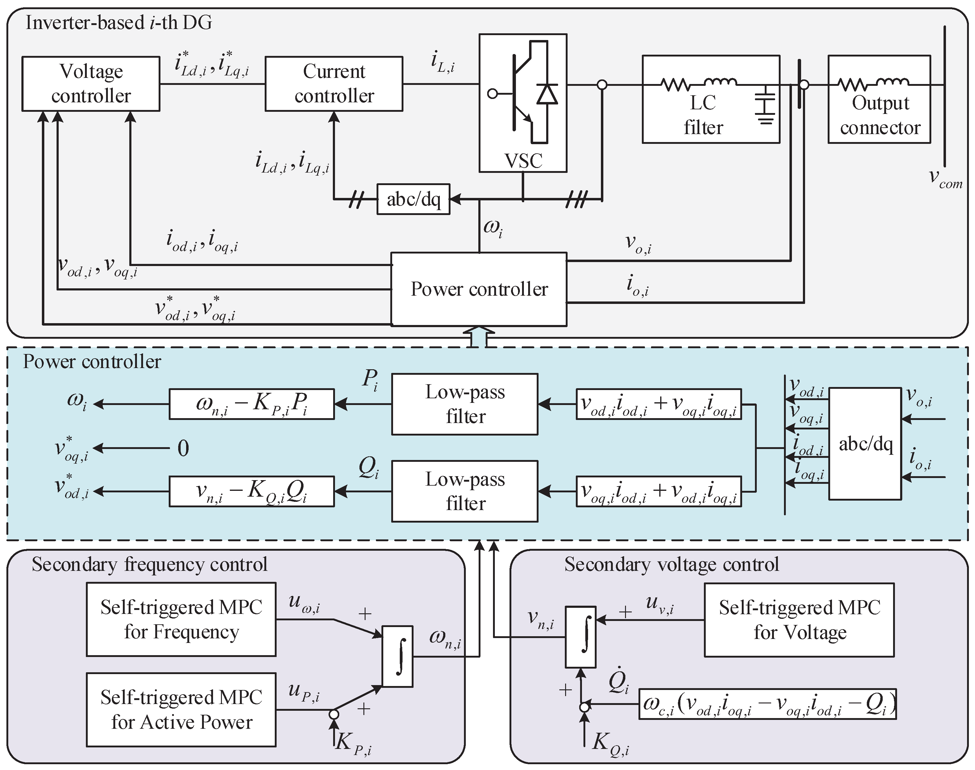
Figure 3.
The voltage under the different states of control input: (a) ; (b) ; (c) .
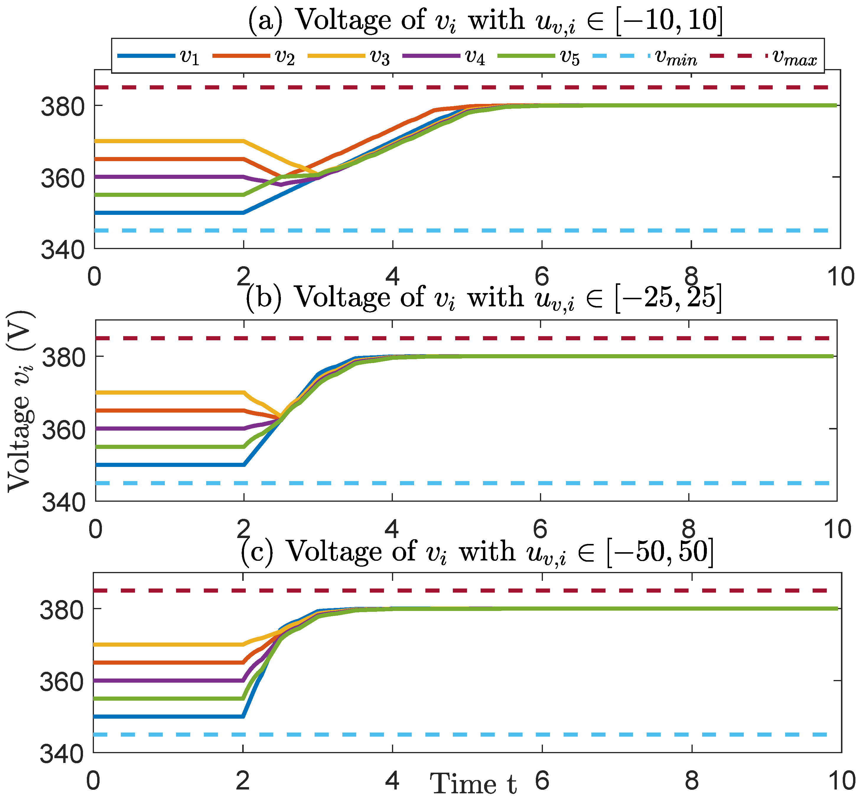
Figure 4.
The frequency under the different states of control input: (a) ; (b) ; (c) .

Figure 5.
The power under the different states of control input: (a) ; (b) ; (c) .
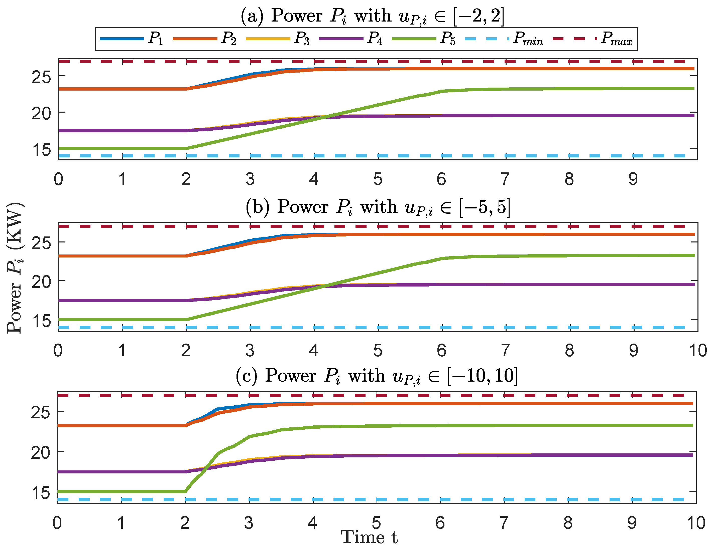
Figure 6.
The self-triggered time of the voltage, frequency and power, respectively: (a) the voltage ; (b) the frequency ; (c) the power .
Figure 6.
The self-triggered time of the voltage, frequency and power, respectively: (a) the voltage ; (b) the frequency ; (c) the power .

Table 1.
Parameters of the AC microgrid.
| Parameter | |||||
|---|---|---|---|---|---|
| = 0.35 mH | = 0.03 | = 0.1 mH | = 1.35 mH | = 0.1 mH | = 50 F |
| Parameter | Load 1 | Load 2 | |||
| (per phase) | 12 kW | 15.3 kW | |||
| (per phase) | 12 kVAr | 7.6 kVAr | |||
| Parameter | Line 1 | Line 2 | Line 3 | ||
| 0.23 | 0.35 | 0.23 | |||
| 318 H | 1847 H | 318 H |
Table 2.
Parameters of the self-triggered MPC control.
| Parameter | |||||
|---|---|---|---|---|---|
| 0.75 | 0.5 | 0.7 | 0.6 | 0.8 | |
| T = 0.05 s | K = 2 | = 10 | |||
| Parameter of | Q = 10 | R = 1 | = 380 V | ||
| Parameter of | Q = 15 | R = 2 | = 314 (rad/s) | ||
| Parameter of | Q = 6 | R = 1 | = 26 kW |
Publisher’s Note: MDPI stays neutral with regard to jurisdictional claims in published maps and institutional affiliations. |
© 2022 by the authors. Licensee MDPI, Basel, Switzerland. This article is an open access article distributed under the terms and conditions of the Creative Commons Attribution (CC BY) license (https://creativecommons.org/licenses/by/4.0/).
Share and Cite
MDPI and ACS Style
Dong, X.; Gan, J.; Wu, H.; Deng, C.; Liu, S.; Song, C. Self-Triggered Model Predictive Control of AC Microgrids with Physical and Communication State Constraints. Energies 2022, 15, 1170. https://doi.org/10.3390/en15031170
AMA Style
Dong X, Gan J, Wu H, Deng C, Liu S, Song C. Self-Triggered Model Predictive Control of AC Microgrids with Physical and Communication State Constraints. Energies. 2022; 15(3):1170. https://doi.org/10.3390/en15031170
Chicago/Turabian StyleDong, Xiaogang, Jinqiang Gan, Hao Wu, Changchang Deng, Sisheng Liu, and Chaolong Song. 2022. "Self-Triggered Model Predictive Control of AC Microgrids with Physical and Communication State Constraints" Energies 15, no. 3: 1170. https://doi.org/10.3390/en15031170
Note that from the first issue of 2016, this journal uses article numbers instead of page numbers. See further details here.