
Harmonics and Interharmonics Detection Based on Synchrosqueezing Adaptive S-Transform


Key Lab of Power Electronics for Energy Conservation and Motor Drive of Hebei Province, Yanshan University, Qinhuangdao 066004, China
*
Author to whom correspondence should be addressed.
Energies 2022, 15(13), 4539; https://doi.org/10.3390/en15134539
Submission received: 20 May 2022
/
Revised: 12 June 2022
/
Accepted: 17 June 2022
/
Published: 21 June 2022
(This article belongs to the Special Issue Active Power Filters and Power Quality)
Abstract
:The integration of renewable energy generation and nonlinear power electronic equipment into the grid brings about complex harmonics and interharmonics problems. The amplitude and frequency of harmonics and interharmonics should be detected by high time-frequency (T-F) resolution methods owing to their time-varying transient features. In this paper, a synchrosqueezing adaptive S-transform (SAST) method is proposed to detect the parameters of harmonics. Firstly, the time-frequency spectrum (TFS) of the harmonic signals is acquired by an adaptive S-transform (AST) algorithm. The TFS results are then subjected to synchronous compression, so as to achieve higher time-frequency representation precision. The detection results of the simulation signals show that SAST can achieve a better time-frequency resolution than the S-transform (ST) and synchrosqueezing short-time Fourier transform (SSTFT). In addition, the application of SAST to the analysis of experimental signals also suggests its superiority in the parameter detection of harmonics, especially for the time-varying interharmonics.
1. Introduction
With a high proportion of new energy generation and nonlinear power electronics connected to the grid, the impact of harmonics and interharmonics on power quality is of increasing concern [1]. Harmonics represent grave hazards, such as motor noise, voltage deviation and resonance for transformers, motors, arc furnaces, metering instruments and other industrial equipment [2,3,4]. Moreover, harmonics can also result in grid-voltage fluctuations as well as the flicker, resonance, and over-zero shifts in the voltage waveform [5,6]. Therefore, the detection and analysis of harmonics and interharmonics are of great significance to promote the safety and power quality of new energy generation.
In a power system, an AC non-sinusoidal signal can be decomposed into linear combinations of sinusoidal components of different frequencies. When the frequency of the sinusoidal component is the same as the frequency of the original AC signal, it is called fundamental. When the frequency of the sinusoidal component is an integer multiple of the frequency of the original AC signal, it is called a harmonic [7,8,9]. For example, if the frequency is three times, five times, or seven times the fundamental frequency, the harmonic is called the third harmonic, fifth harmonic, or seventh harmonic. When the frequency of the sinusoidal component is a non-integer multiple of the frequency of the original AC signal, it is called an interharmonic. For example, when the frequency is 1.5 times or 2.5 times the fundamental frequency, the signal is called interharmonic at this time [10]. Due to the large number of nonlinear loads connected to the grid, this can lead to serious harmonic problems. When these nonlinear loads are impulsive, the nonlinear fluctuating loads will create serious interharmonic problems [11,12]. Harmonics and interharmonics can cause serious interference phenomena in power systems. For example, it causes abnormal vibration in induction motors. The traditional signal detection methods are not accurate enough for harmonics and interharmonics, and thus cannot effectively analyze power quality problems [13].
The conventional harmonic and interharmonic detection methods mainly include short-time Fourier transform (STFT) [14], wavelet transform (WT) [15], Hilbert–Huang transform (HHT) [16,17,18], and S-transform (ST) [19,20]. In [21], STFT was used to detect harmonics. The analysis results of the integer harmonics revealed a high accuracy of STFT, however, STFT had the defects of frequency leakage due to asynchronous transformations. The harmonic detection by WT indicated that the wavelet basis of WT substantially influenced the detection results [22]. When ST was used to detect harmonics, the window function of ST had a fixed tendency to vary and it failed to achieve the best resolution [23]. The HHT algorithm was proven to be particularly effective in dealing with nonlinear and non-smooth signals, and it required no basis function prior to computation. However, HHT showed poor noise immunity, which was attributed to its high sensitivity to noise [24]. It was demonstrated by some scholars that the MUSIC and time-frequency adaptive atoms could well improve the time-frequency resolution [25]. A great many researchers claimed that synchronous squeeze transform (SST) could effectively improve the detection accuracy of harmonics. In a number of studies, the combined methods of WT, ST and SST for harmonic detection [26] greatly enhanced the time-frequency resolution, which, however, was still affected by the wavelet basis and the window function of ST. A generalized S-transform-based SST (GSST) algorithm [27] was proposed to improve the window function of ST, but its computation was intricate because its parameters were acquired iteratively.
To tackle the above-mentioned problems, a synchrosqueezing adaptive S-transform (SAST) method was developed to detect the parameters of harmonics and interharmonics in this article. An adaptive S-transform (AST) algorithm was designed at first to provide a TFS with an adequate resolution for SST. The time-frequency resolution was obtained by direct optimization of the standard deviation of the window function without iterative calculation. Secondly, a SAST was adopted to further improve the time-frequency resolution. Due to the continuous distribution of the time-varying harmonic components in the frequency domain, the best time-frequency resolution cannot be achieved only by optimizing the window function of AST. The TFS of AST near the instantaneous frequency of SAST was squeezed onto that frequency, which improved the time-frequency resolution of SAST for detecting harmonics and interharmonics.
The main contribution of SAST is that it directly matches a Gaussian window with the main value interval of the power quality signal spectrum to optimize the time-frequency resolution. The optimization was based on the three sigma criterion, and the best value of the standard deviation of the Gaussian window was sought directly through the energy occupation ratio. Hence, the traditional multi-parameter iteration problem was eliminated and the time-frequency resolution was improved. Moreover, SAST was less affected by noise compared with the other harmonic detection algorithms. By the end of the paper, the method was compared with the existing harmonic detection methods in the analysis of mathematical model signals and the signals generated by the simulation platform. The analysis results verified the detection accuracy and noise immunity of the proposed method.
2. Synchrosqueezing Adaptive S-Transform Theory
Developed from STFT, the traditional ST converts the standard deviation of the window function into a frequency function. The traditional ST [28] of the signal is defined as
in which , and represent the time, frequency and time-shift factors, respectively. The time factor controls the position of the window function on the time axis, thus ensuring that the window function can analyze the entire time horizon.
The window function of traditional ST is:
The corresponding standard deviation is:
Although ST inherits the advantages of STFT and WT, the fixed trend of varying with the frequency deteriorates the time-frequency resolution of ST, according to (3). Therefore, an AST algorithm is built to afford the TFS of the harmonic signal. The time-frequency resolution of AST can be adjusted by changing the standard deviation .
The window function of AST can be written as
in which the value interval is completely determined by the spectrum of the signal .
The corresponding AST is:
Comparing Equations (1) and (2), the standard deviation is no longer a fixed function of frequency . The window function is indirectly related to frequency.
To determine the value interval of standard deviation , a window matching spectrum (WMS) method is designed as follows.
The window function of AST is represented in the frequency domain as
The effective window width can be defined based on the frequency domain extension of the window function:
According to Equation (8), the frequency domain expansion is inversely related to the standard deviation . The effective window width can be defined based on the criterion when it covers the main energy distribution of the window function centered on the frequency point.
Substituting into Equation (7), we have
When , the amplitude of the Gaussian window function is only 0.0111, and 99.73% of the energy distribution of the Gaussian window function is included. Therefore, the effective window width of the Gaussian window can be expressed as
where the frequency point corresponding to the effective window width of the window function is:
Therefore, these frequency points have a reciprocal relationship with the standard deviation .
To avoid energy leakage and frequency aliasing, the effective window width should cover the major energy distribution of the frequency component but not the energy distribution of its adjacent frequency components and .
The spectrum energy of each frequency component is represented as
in which and . There is a frequency interval that makes the main energy satisfy
The frequency interval denotes the frequency main energy interval, which contains more than a 99% energy distribution of the frequency component . To eliminate feature information loss and frequency aliasing, the effective window width of the Gaussian window should cover the main energy interval of the frequency component , but its adjacent intervals and need to be excluded.
For interharmonic signals, the time-varying harmonic components are continuously distributed in the frequency domain, and their main energy interval becomes invalid. However, the main energy interval of the fundamental frequency components is still useful to determine the standard deviation .
Therefore, the frequency coordinates of the effective window width corresponding to the fundamental frequency component should satisfy
The value of corresponding to the frequency component is calculated as
in which corresponds to the best time resolution, and denotes the best frequency resolution.
The obtained value interval of is used to improve the time-frequency resolution of AST. This method is free of frequency aliasing and iterative calculations. However, on account of the continuity of time-varying harmonics, AST is unable to achieve the best energy concentration through the WMS method. Therefore, a SAST algorithm is established based on the TFS of AST to further improve the time-frequency resolution.
Synchrosqueezing is to squeeze energy into the real instantaneous frequency of the signal. The derivation process of SAST is briefly introduced as:
Let , AST can be expressed as:
According to the synchrosqueezing wavelet transform [29], the signal function also adopts a single frequency function
Bringing Formula (19) into Formula (17), we have
By deriving the spectrum during AST transformation, the instantaneous frequency is estimated. Formula (20) is the result of deriving the time factor
The instantaneous frequency of the signal is computed by deriving the time spectrum of AST.
The SAST algorithm rearranges the frequency spectrum of AST and squeezes the energy of the center frequency to the position of . The SAST formula of can be thus expressed as
in which is the instantaneous frequency, is the center frequency and is the discrete frequency.
The above is the theoretical introduction of SAST. The criterion is applied to the window function of the Gaussian window, and the window width is directly matched with the energy range of the signal to determine the best . Unlike ST, AST dispenses with the need for frequency aliasing, Furthermore, AST provides a TFS with an adequate resolution for SST. The succeeding SST treatment renders the energy distribution of the harmonics and interharmonics more concentrated, and a satisfactory time-frequency resolution is finally achieved.
3. Performance Analysis
The merging of a large number of new energy sources, such as wind power and photovoltaic power into the grid, gives rise to a growing prominence in harmonics and interharmonics issues. The detection of harmonics and interharmonics parameters is extremely important for harmonic control. This section aims to detect the harmonic and interharmonic parameters. To verify its effectiveness, SAST is compared with the other approaches to their analytical results of different signals (mathematical models, noise signals, signals generated by new energy sources connected to the grid and experimental platforms).
3.1. Time-Frequency Analysis Performance Comparison Based on Mathematical Models
The proposed method is tested on time-varying harmonic signals, and the experimental results are compared with those of SSTFT, HHT, WT and ST. The simulation experiments are conducted in a MATLAB environment with a signal sampling rate of 1600 Hz. The test signal is described as:
According to Equation (24), the test signal contains components with different frequencies and amplitudes. The frequencies of interharmonics are 75 Hz, 110 Hz, 140 Hz and 350 Hz, and the corresponding amplitudes are 0.8, 0.6, 0.4 and 0.6, respectively.
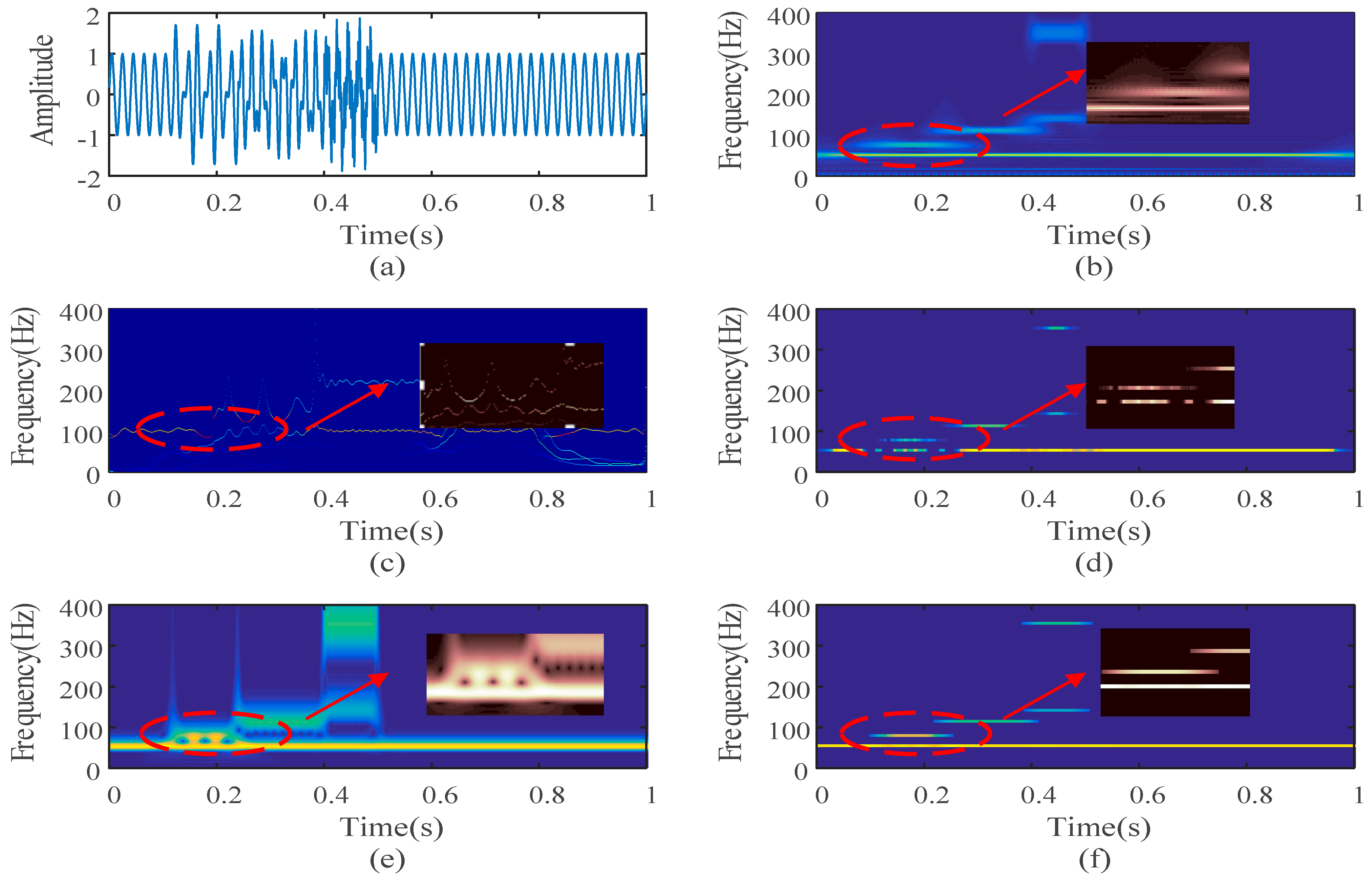
Figure 3 shows the comparison results of the five methods. As can be seen from Figure 3e, ST has the worst time-frequency resolution and cannot effectively distinguish between the five frequency contents. Because the window function of ST is frequency-dependent only, this single trend of variation causes the lack of resolution accuracy of ST and thus cannot distinguish the signals effectively. The time-frequency plot of HHT contains the information that is related to the instantaneous frequency. However, it can be seen from Figure 3c that the analysis of HHT is poor. Because of the endpoint effect of HHT, for the time-varying interharmonics, the signal at the time-varying endpoints produce misalignment. Therefore, it causes poor discrimination. WT can effectively distinguish the five frequency contents, however, the energy concentration is poor compared with SSTFT and SAST. This is influenced to some extent by the wavelet base. Compared with the other three methods, SSTFT and SAST are better, with SAST being the best due to the higher matching of the window function to the signal in SAST compared with SSTFT, which improves the time-frequency resolution. Therefore, SAST has a better analysis for time-varying interharmonics.
Compared with ST, WT and HHT, SSTFT and SAST have better analysis results. To further compare the analytical accuracy of the two, the detection accuracies of the two methods in terms of the frequency and amplitude are listed in Table 1. SSTFT can detect all the frequency components, showing a high detection accuracy for the frequency. However, the amplitude’s relative error of the 75 Hz component detected by SSTFT is 19.43%, which does not satisfy the detection accuracy requirement. SAST has the highest detection accuracy for both the frequency and amplitude, proving that SAST has a high time-frequency resolution and can effectively detect the harmonic components.
The temporal resolution of the two methods is further analyzed by this experiment. The detection accuracies of the three methods in the time domain are listed in Table 2.
In Table 2, the accuracy analysis was performed separately for the start and end times. As shown in Table 2, SSTFT has the lowest temporal resolution, which is due to the problem of the low temporal resolution of STFT itself, which is influenced by the window function. In contrast, SAST has the highest temporal resolution because the window function of SAST is determined according to the 3sigma criterion, which enhances the analysis accuracy to some extent.
3.2. Anti-Noise Analysis of Signals Based on Mathematical Models
To further test the anti-noise performance of SAST, simulation experiments were conducted on noisy signals in a MATLAB environment at a signal sampling rate of 512 Hz, and the results were compared with other time-frequency analysis methods (ST, WT, HHT and SSTFT). The mathematical model of the signal is:
The two signals of different frequencies were superimposed, to which the Gaussian white noise with a signal-to-noise ratio of 10 dB was added. The experimental results are shown in Figure 4.
It can be seen from Figure 4c that HHT suffers modal aliasing in a strong noise environment and cannot identify the signal clearly. This indicates that the HHT performs poorly in terms of noise immunity. Because HHT analyzes the signal through the EMD decomposition process, EMD is analyzed by forming an upper and lower envelope for the very large and very small values, and the noise environment easily affects the accuracy of the upper and lower envelopes. Thus, the resolution accuracy of HHT in a noisy environment is not high. Figure 4b,e are the analyses of WT and ST. Both have a poor resolution in noisy environments. This is because the window function of ST is not matched enough, while WT is affected by the wavelet basis and the number of decomposition layers. According to the figures, the time-frequency analyses of SSTFT and SAST have higher resolution and a better energy concentration than the other methods. The spectral energy of the other approaches is distributed in a more dispersed way than that of SAST. It indicates that these two algorithms have better anti-noise capabilities in harmonic detection. However, the energy distribution of SAST is more concentrated than that of SSTFT. In summary, SAST has better noise immunity.
To further examine the consistency between the analytical results of SAST and the original signal, the estimated instantaneous frequencies of the simulation results were compared with the true instantaneous frequencies of the signal. The values of some of the true frequencies and estimated frequencies are also listed and written in Table 3 swell, so that a more visual comparison can be made.
It can be inferred from the coincidence degree of the two types of frequencies that the estimated value of SAST is highly accurate, which further confirms the effectiveness of this method.
3.3. Time-Frequency Parameters Analysis Based on New Energy
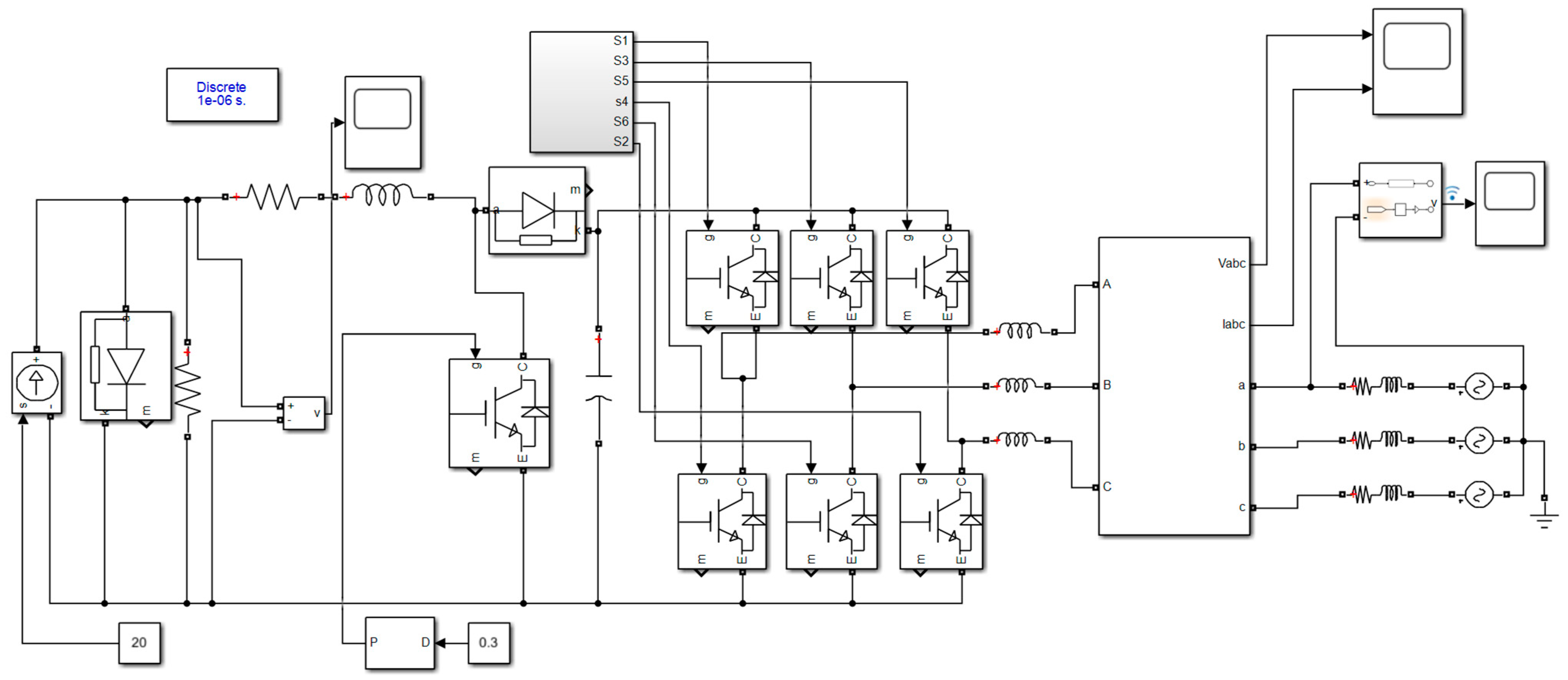
In this section, the resolution of SAST was checked on the harmonic signals, which were generated by the grid connection of new energy. The photovoltaic grid-connected inverters are one of the main harmonic sources in the power grid. Another origin of harmonics is the large-scale wind power grid-connected systems. Therefore, it is essential to attest to the effectiveness of SAST on the photovoltaic grid connection and wind power grid connection models. Firstly, a photovoltaic grid-connected inverter model (Figure 5) was built for comparison and verification. Additionally, it gave the individual parameters of the PV grid-connected inverter model in Table 4.
Since the mathematical model of the acquired signal was unknown, the fast Fourier transform (FFT) of the acquired signal was performed to yield the frequency components and bandwidth of the signal. According to the FFT results of the signal, the frequency components of the signal were 50 Hz, 100 Hz, and 150 Hz … The fundamental frequency of the signal was 50 Hz, the maximum frequency was 750 Hz, and the frequency bandwidth was 700 Hz. The FFT results provided a reference for the comparison of the experimental results.
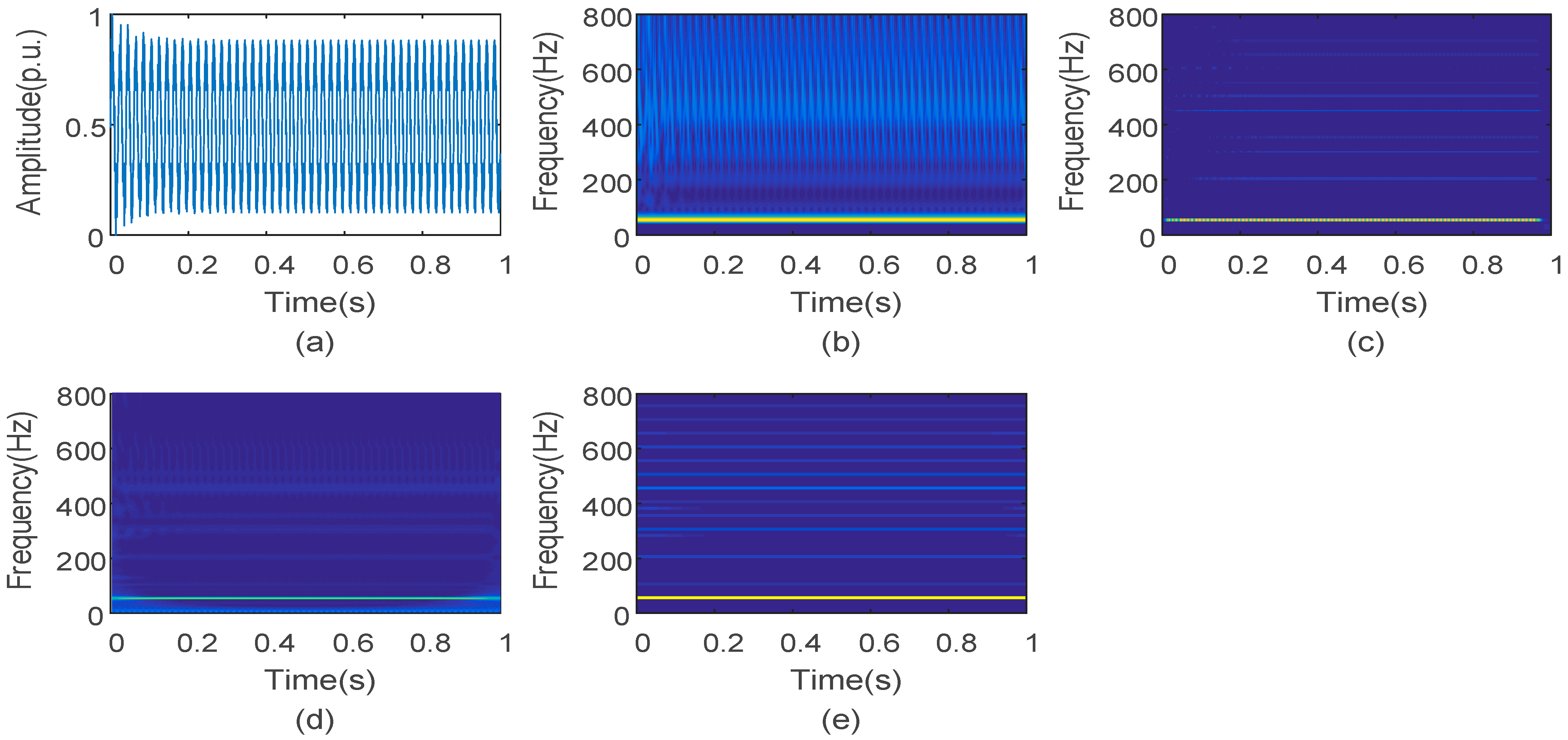
In order to facilitate the analysis, the amplitude of the harmonic signals generated by SAST was normalized to [−1,1]. The sampling rate of the signal was 1600 Hz, and the experiment was conducted in a MATLAB environment. Figure 6 is the time-frequency spectra of ST, SSTFT, WT and SAST.
It can be seen from Figure 6b,d that the harmonic and interharmonics, except for the fundamental frequency of the analog signal, are severely ambiguous, implying that the T-F resolutions of ST and WT are not adequate for the detection of parameters. The single nature of the window function and the fixed nature of the wavelet basis were the main reasons for the lack of accuracy of ST and WT for the interharmonic analysis. In Figure 6c, the TFS of SSTFT is better than that of ST due to the “squeezing” effect, however, SSTFT sustained a huge energy loss. As for SAST in Figure 6e, there is no energy loss in the TFS, and each frequency component can be clearly recognized. The results demonstrated that the time-frequency resolution of SAST was higher than that of the ST, WT and SSTFT. Because SAST matched the signal components by the 3sigma criterion, the harmonics and interharmonics could be analyzed more effectively
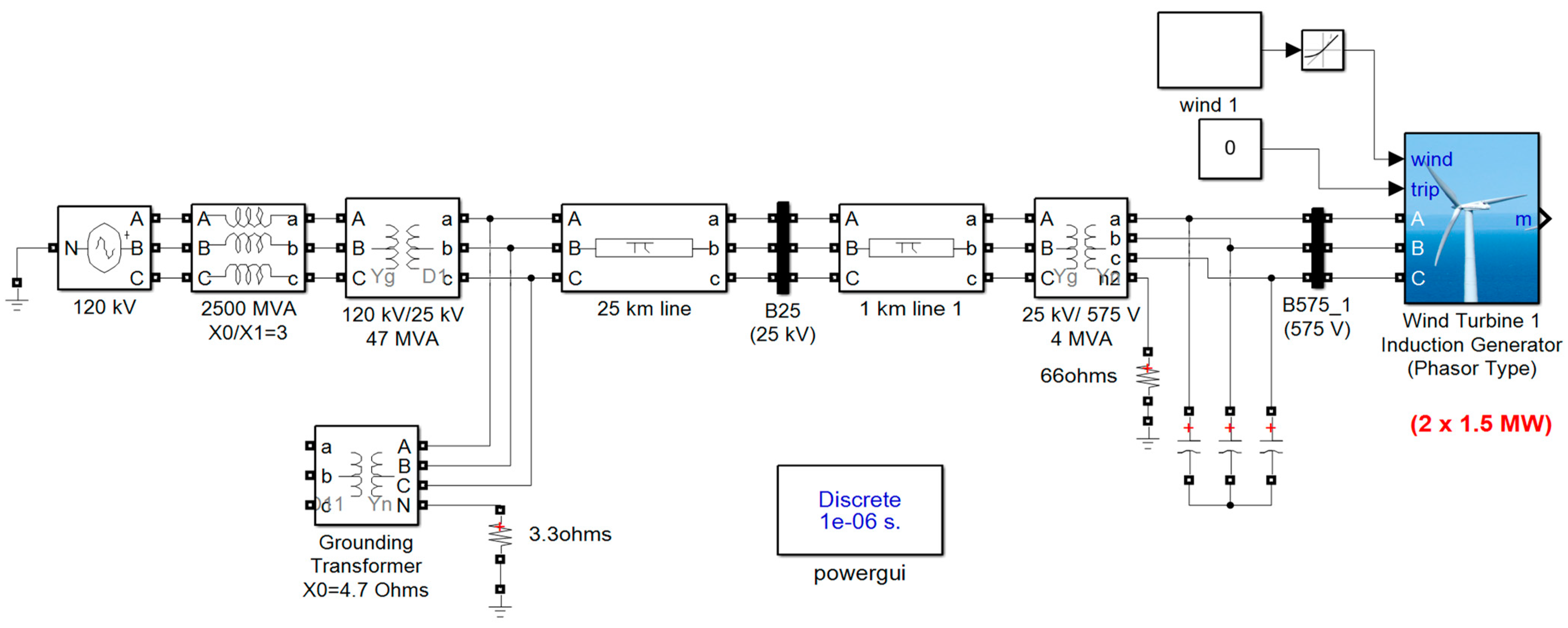
Secondly, the wind power grid-connected system model was established to simulate the interharmonic signal, and the detection accuracy of SAST was further verified in this model. In the simulation verification process, both the video analysis diagrams and detection results of the various parameters were analyzed to check the analysis error. The simulation experiment was still conducted in a MATLAB environment at a signal sampling rate of 1600 Hz. The grid-connected system of wind power generation is shown in Figure 7. SAST was applied to analyze the wind power grid-connected signals, and its effectiveness in separating the different frequency components was measured. Additionally, it gave the individual parameters of the wind power grid in Table 5.
The same FFT was performed on the signal to afford the frequency components and bandwidth, and the FFT results contributed to the comparison of the experimental results. The FFT results showed that the frequency components of the signal were 50 Hz, 100 Hz, 150 Hz …, 750 Hz. The signal had a fundamental frequency of 50 Hz, a maximum frequency of 750 Hz, and a frequency bandwidth of 700 Hz.
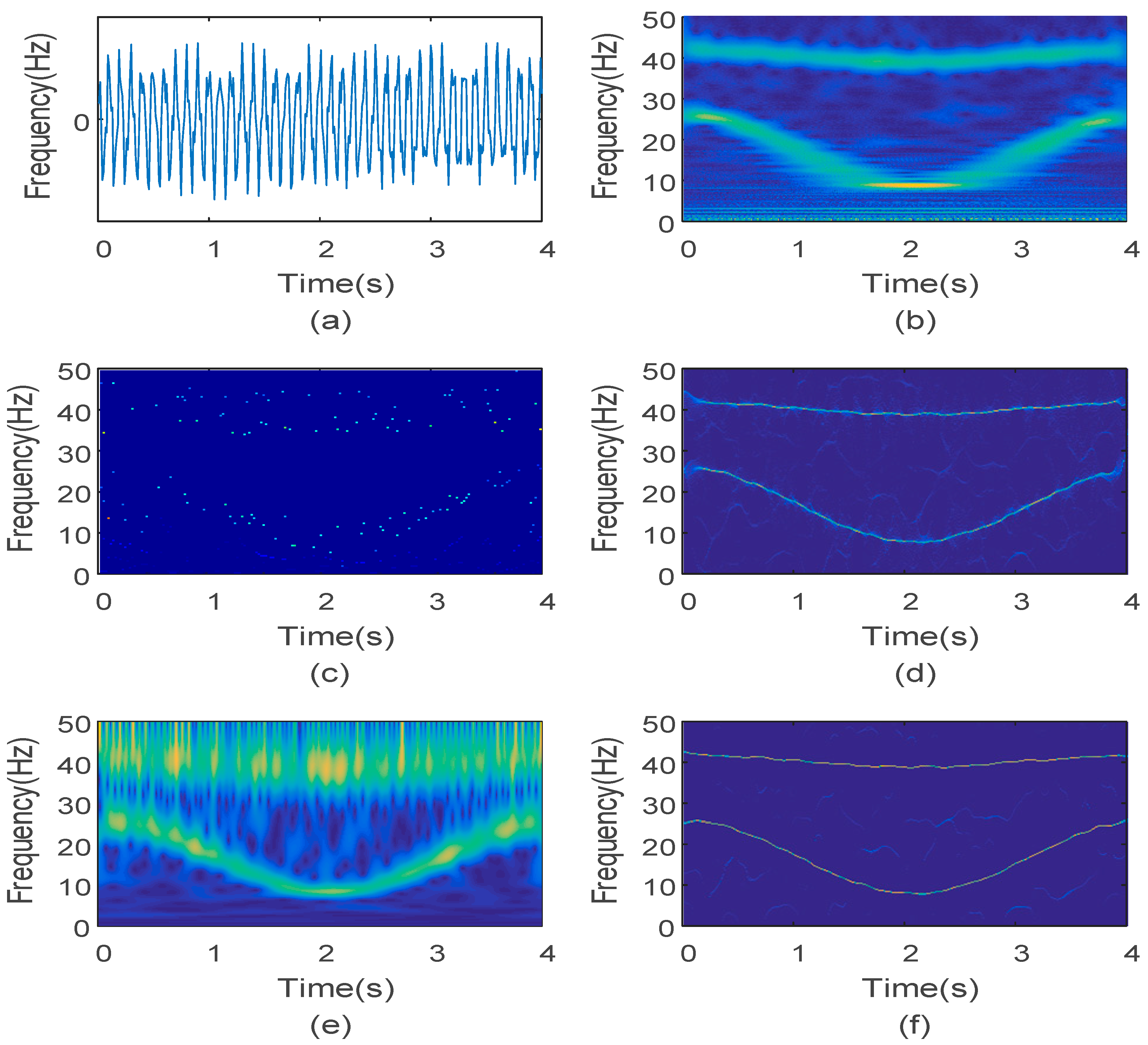
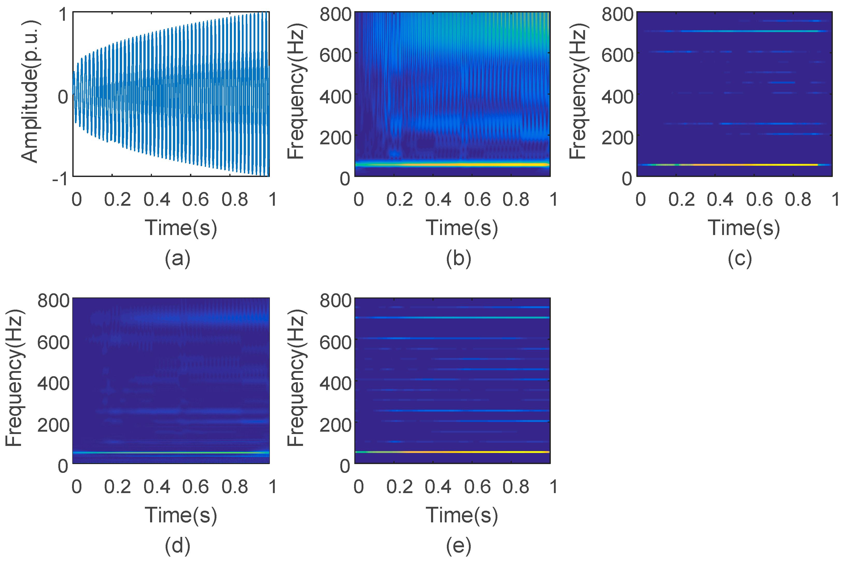
Similarly, the interharmonic signal data generated by this model were normalized to [−1,1]. The time-frequency spectra of ST, SSTFT, WT and SAST are presented in Figure 7. Figure 8a–e are the TFSs of the original signal, ST, SSTFT, WT and SAST, respectively. As shown in Figure 8, the frequency components of the T-F plots that were generated by the ST method and WT method are blurred, which is attributed to the low T-F resolution. Owing to the “squeezing” effect, the SSTFT and SAST methods have a higher T-F resolution than the ST method. Comparing Figure 8c,e, SSTFT and SAST have a similar frequency resolution, however, SAST suffers less energy loss than SSTFT, suggesting that the T-F resolution of SAST is better than the other methods. Therefore, SAST has a high T-F resolution to detect the interharmonic parameters. The time-frequency resolution accuracies of ST and WT were affected by the window function and wavelet basis, respectively. In addition, the resolution accuracy of WT was also affected by the number of decomposition layers. SSTFT did not have a high resolution accuracy for the small amplitude signals and could not effectively detect the low amplitude components. SAST improved the analysis accuracy of the interharmonics after the effective matching of window functions and could effectively detect each simple harmonic component.
The interharmonic parameters extracted by SSTFT and SAST are listed in Table 6. SSTFT could identify all the interharmonic components, however, its relative errors were larger than those of SAST. Nevertheless, SAST was capable of identifying all the harmonic components more accurately than the other methods. Taken above, compared with the SSTFT, the SAST method has the highest T-F resolution to detect the parameters of interharmonics.
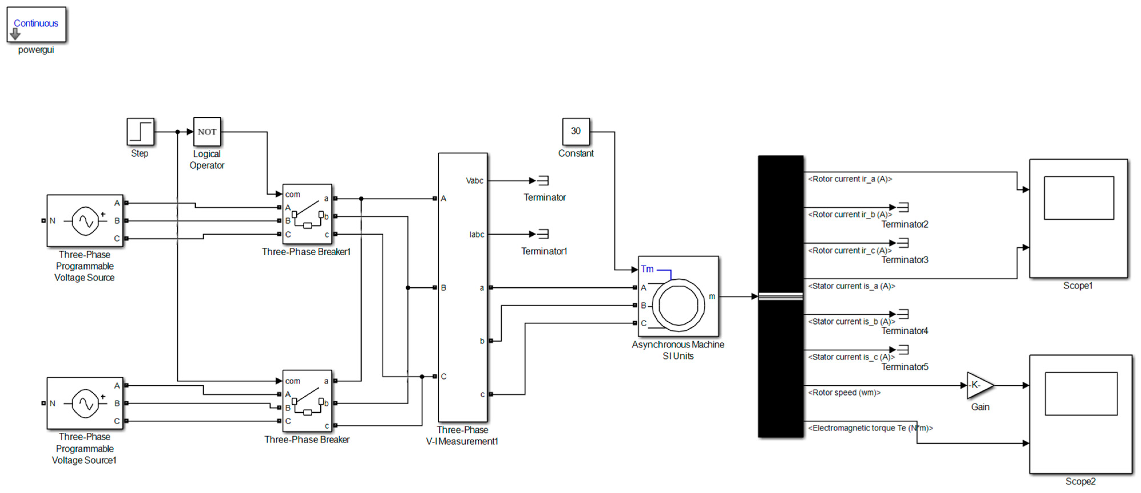
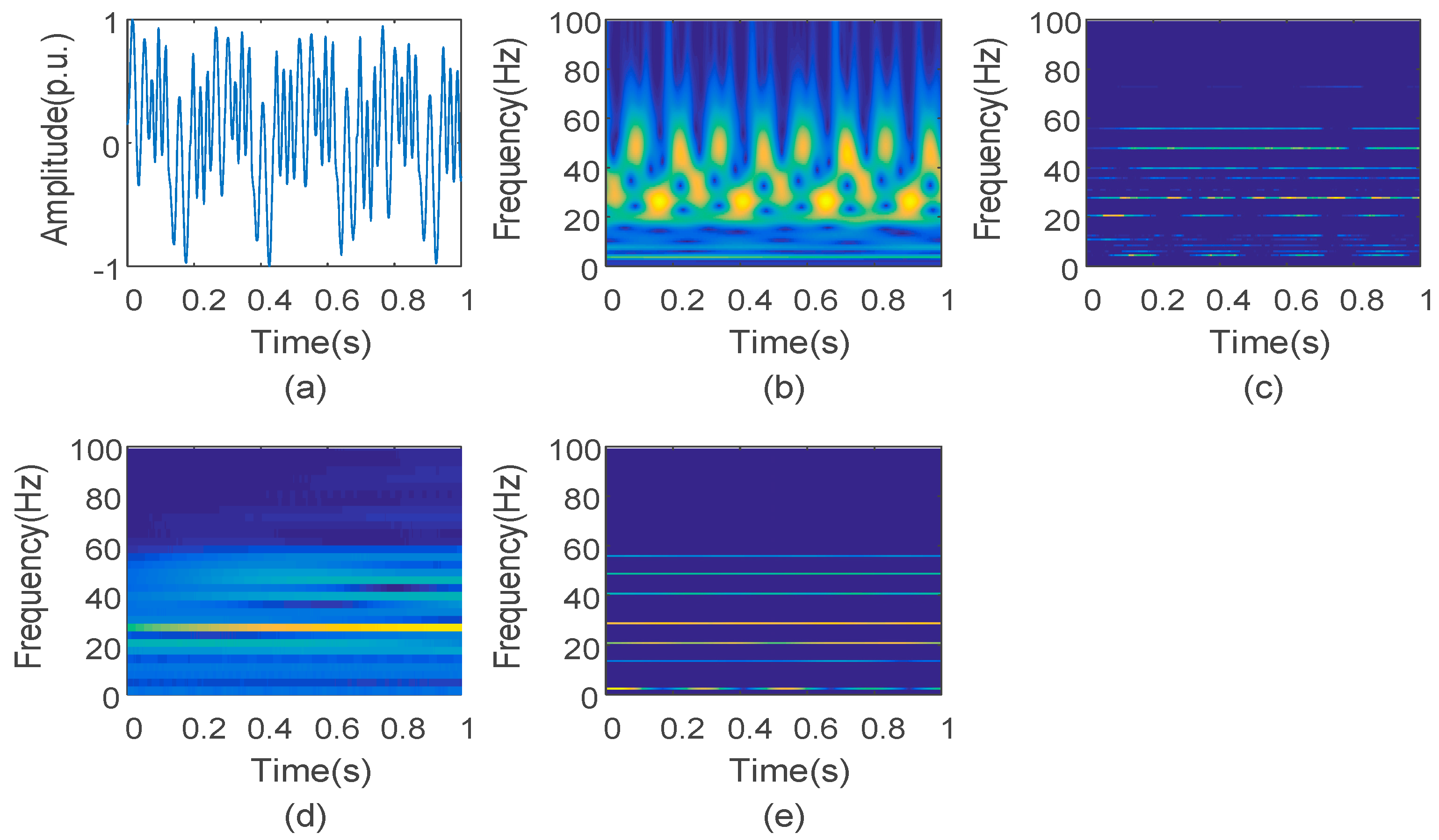
To further illustrate the effectiveness of the method, a model of the induction motor powered by the inverter was built, and the model was built as shown in Figure 9. The relevant parameters of the modified model are also given. Two sets of AC voltage sources with different power supply frequencies with circuit breakers were used to establish the motor inverter speed control model, where voltage source 1 was set to 260 × sqrt (3) V, 60 Hz, and voltage source 2 was set to 220 × sqrt (3) V, 50 Hz, the switching frequency of the two voltage sources was 10 Hz, and the load torque of the motor was 20 Nm. The stator current was collected in the experiment, and the current signal was analyzed. The simulation experiments were still performed in a MATLAB environment, and the sampling rate of the signal was 600 Hz. Additionally, in order to provide a reference for the experimental results, the FFT was used to analyze the signal components. The analysis results showed that the main frequency components contained in the signal were: 4 Hz, 8 Hz, 20 Hz, 48 Hz, and 56 Hz, the lowest frequency of the signal was 4 Hz, the highest frequency was 56 Hz, and the bandwidth of the signal was 52. The experimental comparison results are shown in Figure 10.
Figure 10b represents the ST analysis results of the signal. From Figure 10b, it can be seen that the accuracy of the time-frequency analysis of ST is very poor and that the individual frequency components of the signal cannot be identified, and there are serious crossover phenomena between the frequencies. Because the resolution accuracy of ST is determined to some extent by the frequency and cannot be properly adjusted, this makes the analysis boundary between each frequency unclear when ST analyzes the interharmonics containing multiple frequency contents, thus affecting the analysis accuracy. Figure 10c,d represent the results of the SSTFT analysis and WT analysis of the signal, respectively. The analysis results of SSTFT have an energy loss compared with those of SAST, which leads to insufficient clarity of the frequency components. The analytical accuracy of WT was even worse, and the interharmonic components could not be clearly distinguished. This is because when using WT to analyze the signal, the performance of using WT is not good due to the number of decomposition layers and the window function.Furthermore, the process of the SAST analysis provided good time-frequency results for SST due to the high resolution of AST, and the time-frequency results were better and superior after SST squeezing. In other words, SAST has a higher time-frequency resolution in comparison.
3.4. Measurement Experiment Examples
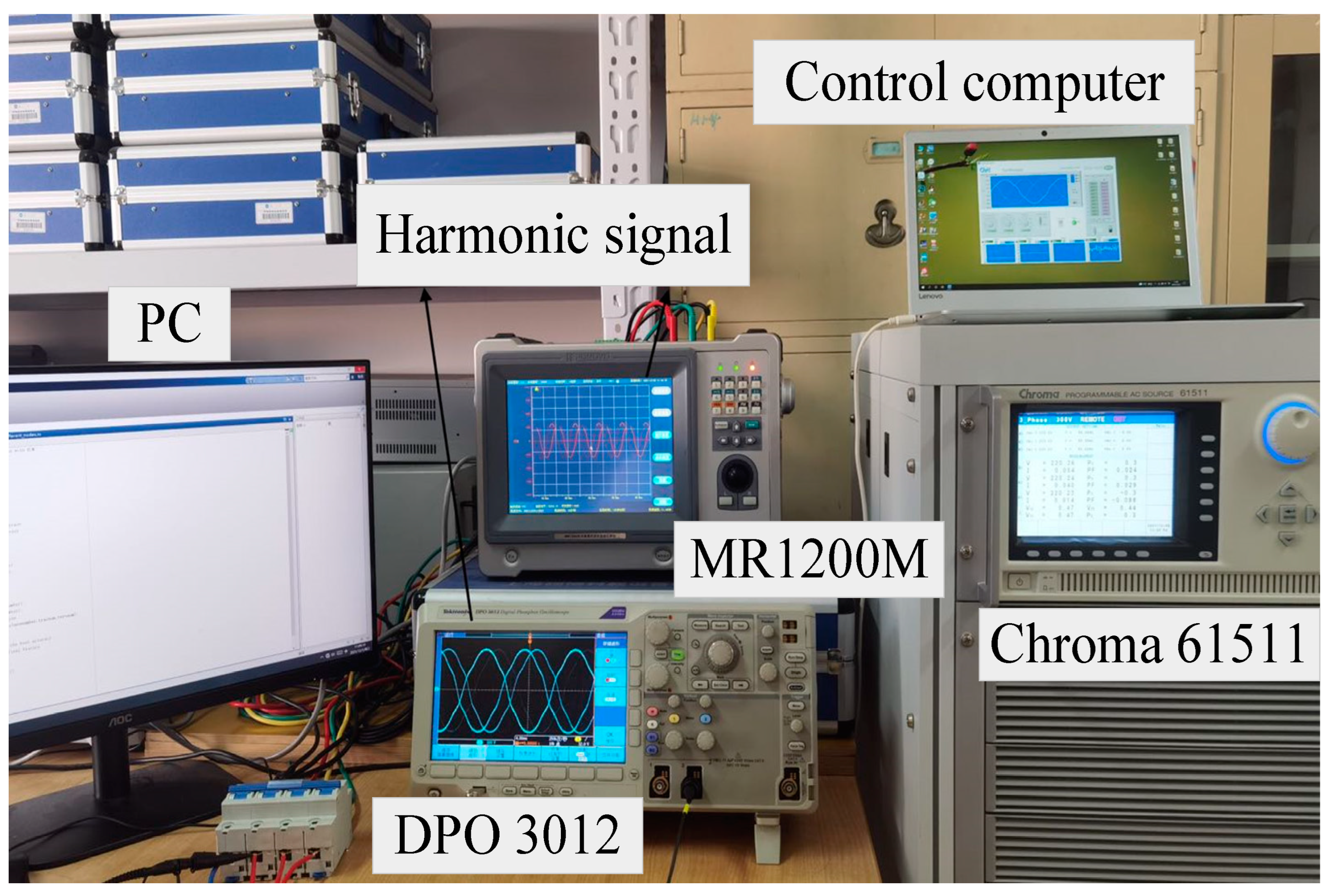
Experimental signals with randomness can better reflect the actual operation of the power system than the simulation signals. In this section, an experimental platform for generating and capturing harmonic and interharmonic signals was built to further authenticate the performance of the proposed method (Figure 11). The hardware platform contained a programmable AC source (Chroma 61511), a control computer, a multi-channel waveform monitoring recorder (MR1200M), a dual-channel oscilloscope (DPO 3012), and a personal computer (PC). The Chroma 61511 was programmed to generate single- or three-phase voltage signals based on the parameters set by the control computer. The MR1200M and DPO 3012 were connected to the Chroma 61511 to sample the experimental signal in real time.
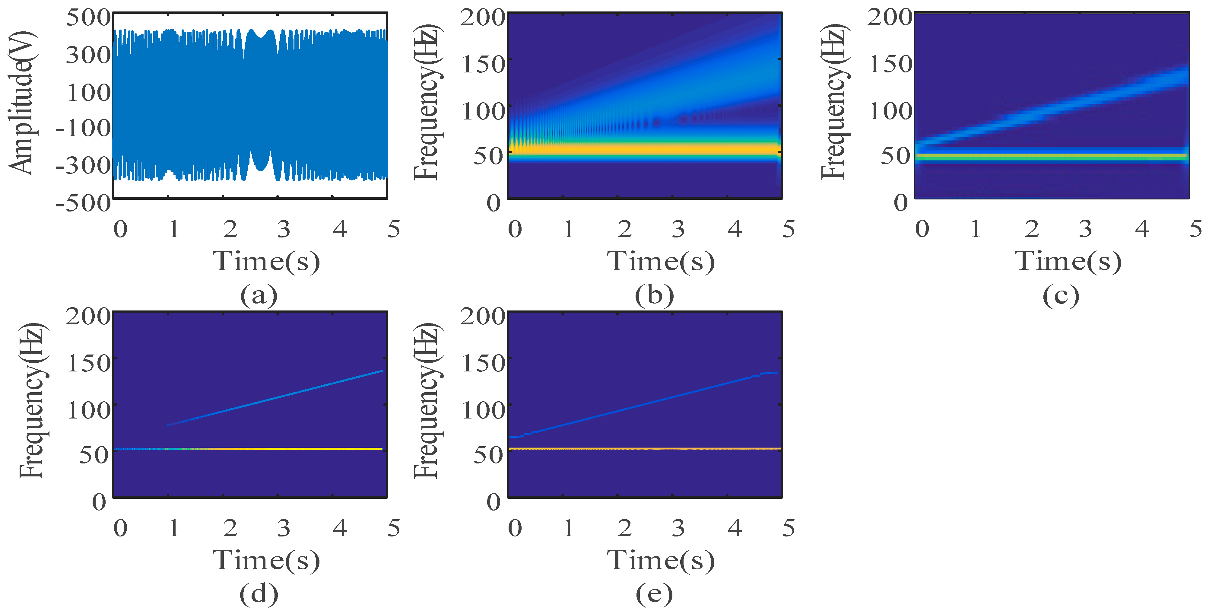
The time-varying interharmonic signal was generated by the programmable AC source Chroma 61511, and then the voltage waveform with the time-varying frequency components was output by the interharmonic module of the instrument. The sampling frequency of the MR1200M was set to 2000 Hz, and the sampling time was 5 s. After sampling the signals, the MR1200M transmitted the signal data to the computer in real time via the universal serial bus interface. The collected interharmonic signal was then analyzed by ST, SSTFT, WT and SAST, and the time-frequency spectra that were yielded are drawn (Figure 12).
In Figure 12, the interharmonic signal contains a fundamental frequency component and a time-varying harmonic component, and the frequency of the latter increases linearly from 60 Hz to 130 Hz. The TFS of ST presents a poor frequency concentration, and the two frequency components in the low-frequency region cannot be separated (Figure 12b). The analysis of WT was improved compared to ST, however, the energy aggregation of the signal performed poorly, as seen in Figure 12c. On the contrary, the T-F spectra generated by SSTFT and SAST had higher frequency concentrations than that of ST. Comparing Figure 12d,e, SSTFT and SAST show a satisfactory time-frequency resolution without frequency aliasing. However, SAST was able to identify the frequency components in the low-frequency region without energy loss. Therefore, SAST is superior to the other methods in the performance of detecting the time-varying experimental signals.
Among the four methods, SSTFT and SAST were better for the analysis. To further compare the analysis results of SSTFT and SAST, Table 7 concludes the accuracy of SSTFT and SAST for detecting the frequency and amplitude of the time-varying harmonic signals. SSTFT was unable to identify the start frequency of the interharmonic signal as a result of the low T-F resolution. For the stop frequency of the interharmonic components, the amplitude relative error of SSTFT was 127.78%, respectively. Thus, the parameter detection result of SSTFT failed to meet the demands. On the contrary, SAST provided an excellent T-F resolution to improve the accuracy of detecting the interharmonic parameters. In addition, for the interharmonic signal with a length of 10,000 points, it only took 2.782 s for SAST to complete the TFA, which is much faster than the ST and SSTFT. Therefore, the SAST method can detect the harmonic parameters with high accuracy and speed.
4. Conclusions
In this study, the SAST method is proposed to analyze and detect harmonics and interharmonics. First of all, an AST algorithm was used to provide a TFS with a moderate resolution for SST. The TFS of AST near the instantaneous frequency of SAST was then squeezed into that frequency, which further improved the time-frequency resolution. The harmonic parameter detection framework, which is based on SAST, was constructed to detect the harmonics and interharmonics. Through the different simulation experiments, SAST was proven to have a higher time-frequency resolution than ST and SSTFT, thus, it can effectively identify the frequency components. This finding is confirmed by the harmonic parameter detection results. Moreover, a measurement experiment example was built, which also verified that SAST had a higher time-frequency resolution when detecting the time-varying experimental signals. The SAST method was highly adaptive to the analysis and parameter detection of the harmonics and interharmonics. Moreover, the parameter detection results of SAST can accurately reflect harmonic characteristics.
The SAST method acts as a powerful tool to analyze harmonic and interharmonic problems under the background of a new energy grid connection.
Author Contributions
Methodology, P.L. and Z.L.; software, P.L.; investigation, P.L., K.M., F.T. and Z.L.; writing—original draft preparation, K.M.; writing—review and editing, K.M. All authors have read and agreed to the published version of the manuscript.
Funding
This work was supported by the National Key R&D Program of China (Grant No. 2021YFB3201600) and The Natural Science Foundation of Hebei Province (E2020203198) and the Cultivation Project for Basic Research and Innovation of Yanshan University (2021LGQN012).
Informed Consent Statement
Formed consent was obtained from all subjects involved in the study.
Conflicts of Interest
The authors declare no conflict of interest.
References
- Zobaa, A.; Aleem, S.A. A New Approach for Harmonic Distortion Minimization in Power Systems Supplying Nonlinear Loads. IEEE Trans. Ind. Inform. 2014, 10, 1401–1412. [Google Scholar] [CrossRef] [Green Version]
- Aleem, S.H.E.A.; Zobaa, A.F.; Balci, M.E.; Ismael, S.M. Harmonic Overloading Minimization of Frequency-Dependent Components in Harmonics Polluted Distribution Systems Using Harris Hawks Optimization Algorithm. IEEE Access 2019, 7, 100824–100837. [Google Scholar] [CrossRef]
- Vivert, M.; Diez, R.; Cousineau, M.; Cobaleda, D.B.; Patino, D.; Ladoux, P. Real-Time Adaptive Selective Harmonic Elimination for Cascaded Full-Bridge Multilevel Inverter. Energies 2022, 15, 2995. [Google Scholar] [CrossRef]
- Göthner, F.; Roldán-Pérez, J.; Torres-Olguin, R.E.; Midtgård, O.-M. Harmonic Virtual Impedance Design for Optimal Management of Power Quality in Microgrids. IEEE Trans. Power Electron. 2021, 36, 10114–10126. [Google Scholar] [CrossRef]
- Sangwongwanich, A.; Blaabjerg, F. Mitigation of Interharmonics in PV Systems With Maximum Power Point Tracking Modification. IEEE Trans. Power Electron. 2019, 34, 8279–8282. [Google Scholar] [CrossRef] [Green Version]
- Sridharan, K.; Babu, B.C. Accurate Phase Detection System Using Modified SGDFT-Based PLL for Three-Phase Grid-Interactive Power Converter During Interharmonic Conditions. IEEE Trans. Instrum. Meas. 2021, 71, 1–11. [Google Scholar] [CrossRef]
- Xiahou, K.S.; Liu, Y.; Wu, Q.H. Robust Load Frequency Control of Power Systems Against Random Time-Delay Attacks. IEEE Trans. Smart Grid 2021, 12, 909–911. [Google Scholar] [CrossRef]
- Delkhosh, H.; Seifi, H. Power System Frequency Security Index Considering All Aspects of Frequency Profile. IEEE Trans. Power Syst. 2021, 36, 1656–1659. [Google Scholar] [CrossRef]
- Roca, D.A.L.; Mercado, P.; Suvire, G. System Frequency Response Model Considering the Influence of Power System Stabilizers. IEEE Lat. Am. Trans. 2022, 20, 912–920. [Google Scholar] [CrossRef]
- Li, Y.; Teng, Z.; Tang, Q.; Ji, Z. Detection of Interharmonics Using Sparse Signal Decomposition Based on ICA-MP. IEEE Trans. Instrum. Meas. 2021, 70, 1–9. [Google Scholar] [CrossRef]
- Peterson, B.; Rens, J.; Botha, G.; Desmet, J. On Harmonic Emission Assessment: A Discriminative Approach. SAIEE Afr. Res. J. 2017, 108, 165–173. [Google Scholar] [CrossRef] [Green Version]
- Mohamadian, S.; Pairo, H.; Ghasemian, A. A Straightforward Quadrature Signal Generator for Single-Phase SOGI-PLL With Low Susceptibility to Grid Harmonics. IEEE Trans. Ind. Electron. 2022, 69, 6997–7007. [Google Scholar] [CrossRef]
- Wang, R.; Huang, W.; Hu, B.; Du, Q.; Guo, X. Harmonic Detection for Active Power Filter Based on Two-Step Improved EEMD. IEEE Trans. Instrum. Meas. 2022, 71, 1–10. [Google Scholar] [CrossRef]
- Lin, H.-C. Inter-Harmonic Identification Using Group-Harmonic Weighting Approach Based on the FFT. IEEE Trans. Power Electron. 2008, 23, 1309–1319. [Google Scholar] [CrossRef]
- Wang, X.; Wang, B.; Chen, W. The Second-Order Synchrosqueezing Continuous Wavelet Transform and Its Application in the High-Speed-Train Induced Seismic Signal. IEEE Geosci. Remote Sens. Lett. 2021, 18, 1109–1113. [Google Scholar] [CrossRef]
- Wang, X.; Li, B.; Liu, Z.; Roman, H.T.; Russo, O.L.; Chin, K.K.; Farmer, K.R. Analysis of Partial Discharge Signal Using the Hilbert–Huang Transform. IEEE Trans. Power Deliv. 2006, 21, 1063–1067. [Google Scholar] [CrossRef]
- Li, Y.; Lin, J.; Niu, G.; Wu, M.; Wei, X. A Hilbert–Huang Transform-Based Adaptive Fault Detection and Classification Method for Microgrids. Energies 2021, 14, 5040. [Google Scholar] [CrossRef]
- Li, D.; Ukil, A.; Satpathi, K.; Yeap, Y.M. Improved S Transform-Based Fault Detection Method in Voltage Source Converter Interfaced DC System. IEEE Trans. Ind. Electron. 2021, 68, 5024–5035. [Google Scholar] [CrossRef]
- Liu, N.; Gao, J.; Zhang, B.; Wang, Q.; Jiang, X. Self-Adaptive Generalized S-Transform and Its Application in Seismic Time–Frequency Analysis. IEEE Trans. Geosci. Remote Sens. 2019, 57, 7849–7859. [Google Scholar] [CrossRef]
- Platas-Garza, M.A.; de la O Serna, J.A. Polynomial Implementation of the Taylor–Fourier Transform for Harmonic Analysis. IEEE Trans. Instrum. Meas. 2014, 63, 2846–2854. [Google Scholar] [CrossRef]
- Wright, P. Short-time Fourier transforms and Wigner-Ville distributions applied to the calibration of power frequency harmonic analyzers. IEEE Trans. Instrum. Meas. 1999, 48, 475–478. [Google Scholar] [CrossRef]
- Barros, J.; Diego, R. Application of the Wavelet-Packet Transform to the Estimation of Harmonic Groups in Current and Voltage Waveforms. IEEE Trans. Power Deliv. 2006, 21, 533–535. [Google Scholar] [CrossRef]
- Dash, P.; Panigrahi, B.; Panda, G. Power quality analysis using s-transform. IEEE Trans. Power Deliv. 2003, 18, 406–411. [Google Scholar] [CrossRef]
- Afroni, M.J.; Sutanto, D.; Stirling, D. Analysis of Nonstationary Power-Quality Waveforms Using Iterative Hilbert Huang Transform and SAX Algorithm. IEEE Trans. Power Deliv. 2013, 28, 2134–2144. [Google Scholar] [CrossRef]
- Zhang, Z.; Zhong, Y.; Xiang, J.; Jiang, Y. Phase correction improved multiple signal classification for impact source localization under varying temperature conditions. Measurement 2020, 152, 107374. [Google Scholar] [CrossRef]
- Testa, A.; Akram, M.F.; Burch, R.; Carpinelli, G.; Chang, G.; Dinavahi, V.; Hatziadoniu, C.; Grady, W.M.; Gunther, E.; Halpin, M.; et al. Interharmonics: Theory and Modeling. IEEE Trans. Power Deliv. 2007, 22, 2335–2348. [Google Scholar] [CrossRef]
- Fourer, D.; Auger, F.; Czarnecki, K.; Meignen, S.; Flandrin, P. Chirp Rate and Instantaneous Frequency Estimation: Application to Recursive Vertical Synchrosqueezing. IEEE Signal Process. Lett. 2017, 24, 1724–1728. [Google Scholar] [CrossRef] [Green Version]
- Wang, Q.; Li, Y.; Chen, S.; Tang, B. Matching Demodulation Synchrosqueezing S Transform and its Application in Seismic Time–Frequency Analysis. IEEE Geosci. Remote Sens. Lett. 2022, 19, 1–5. [Google Scholar] [CrossRef]
- Tian, Y.; Gao, J.; Wang, D. Synchrosqueezing Optimal Basic Wavelet Transform and Its Application on Sedimentary Cycle Division. IEEE Trans. Geosci. Remote Sens. 2022, 60, 1–13. [Google Scholar] [CrossRef]
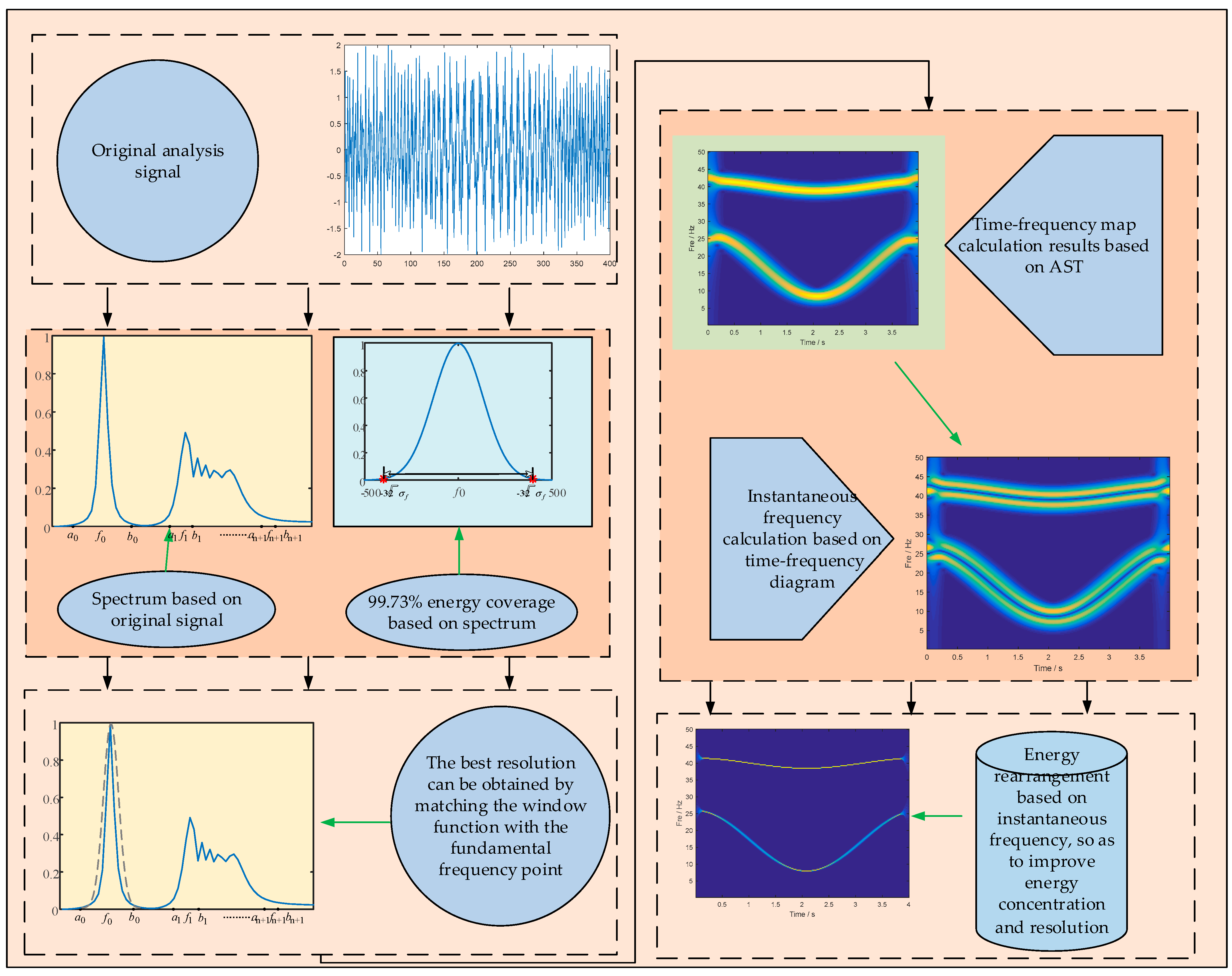
Figure 1.
The schematic diagram of SAST.

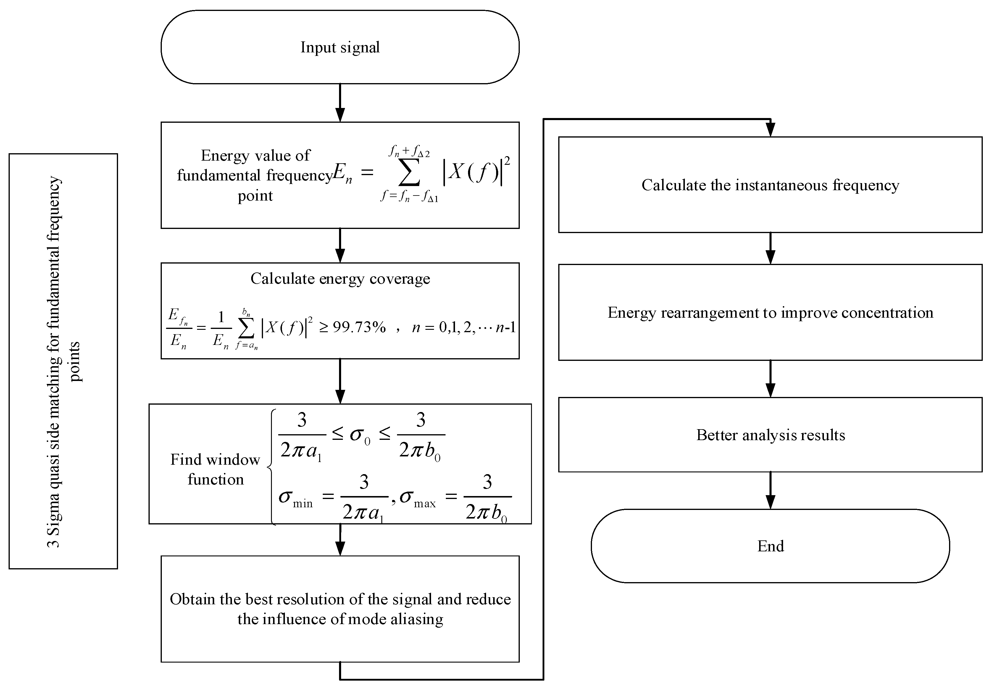
Figure 2.
The flow chart of SAST.

Figure 3.
The results of time-varying interharmonic signals based on five methods. (a) Test signal, (b) WT, (c) HHT, (d) synchrosqueezing STFT (SSTFT), (e) S-transform (ST), (f) synchrosqueezing adaptive S-transform (SAST).
Figure 3.
The results of time-varying interharmonic signals based on five methods. (a) Test signal, (b) WT, (c) HHT, (d) synchrosqueezing STFT (SSTFT), (e) S-transform (ST), (f) synchrosqueezing adaptive S-transform (SAST).

Figure 4.
The results of time-varying harmonic and interharmonic signals based on five methods. (a) Test signal, (b) WT, (c) HHT, (d) SSTFT, (e) ST, (f) SAST.
Figure 4.
The results of time-varying harmonic and interharmonic signals based on five methods. (a) Test signal, (b) WT, (c) HHT, (d) SSTFT, (e) ST, (f) SAST.

Figure 5.
Photovoltaic grid-connected inverter model.

Figure 6.
The time-frequency spectra of photovoltaic grid-connected harmonic signals based on three methods. (a) Simulation signal, (b) S-transform, (c) synchrosqueezing STFT (SSTFT), (d) WT, (e) synchrosqueezing adaptive S-transform (SAST).
Figure 6.
The time-frequency spectra of photovoltaic grid-connected harmonic signals based on three methods. (a) Simulation signal, (b) S-transform, (c) synchrosqueezing STFT (SSTFT), (d) WT, (e) synchrosqueezing adaptive S-transform (SAST).

Figure 7.
Wind power grid-connected model.

Figure 8.
Comparison of wind grid-connected interharmonics based on five time-frequency analysis schemes. (a) The original signal generated by photovoltaic power generation, (b) time-frequency diagram of ST, (c) time-frequency diagram of SSTFT, (d) time-frequency diagram of WT, (e) time-frequency diagram of SAST.

Figure 9.
Inverter induction motor simulation model.

Figure 10.
Simulation comparison of the output current signal of the induction motor based on the inverter power supply. (a) The original signal, (b) time-frequency diagram of ST, (c) time-frequency diagram of SSTFT, (d) time-frequency diagram of WT, (e) time-frequency diagram of SAST.
Figure 10.
Simulation comparison of the output current signal of the induction motor based on the inverter power supply. (a) The original signal, (b) time-frequency diagram of ST, (c) time-frequency diagram of SSTFT, (d) time-frequency diagram of WT, (e) time-frequency diagram of SAST.

Figure 11.
Hardware platform for harmonic signal sampling experiments.

Figure 12.
The time-frequency spectra of experimental interharmonic signals based on three methods. (a) Time-varying interharmonic signal collected by experiment platform (b) S-transform, (c) WT, (d) synchrosqueezing STFT (SSTFT), (e) synchrosqueezing adaptive S-transform (SAST).
Figure 12.
The time-frequency spectra of experimental interharmonic signals based on three methods. (a) Time-varying interharmonic signal collected by experiment platform (b) S-transform, (c) WT, (d) synchrosqueezing STFT (SSTFT), (e) synchrosqueezing adaptive S-transform (SAST).


Table 1.
Accuracy of two methods in detecting time-varying harmonics.
| Test Signal | Actual Value | Detection Value | Relative Error | ||
|---|---|---|---|---|---|
| SSTFT | SAST | SSTFT | SAST | ||
| Harmonic components (Hz) | 50 | 49 | 50 | 2.00% | 0.00% |
| 75 | 74 | 75 | 1.33% | 0.00% | |
| 110 | 109 | 110 | 0.91% | 0.00% | |
| 140 | 139 | 140 | 0.71% | 0.00% | |
| 350 | 349 | 350 | 0.29% | 0.00% | |
| Harmonic amplitudes (V) | 1 | 0.9992 | 1.0040 | 0.08% | 0.40% |
| 0.8 | 0.6446 | 0.8002 | 19.43% | 0.02% | |
| 0.6 | 0.5989 | 0.5962 | 0.18% | 0.63% | |
| 0.4 | 0.3862 | 0.3907 | 3.45% | 2.33% | |
| 0.6 | 0.5712 | 0.5931 | 4.80% | 1.15% | |
Table 2.
Accuracy of time detected by the two methods.
| Test Signal | Actual Value | Detection Value | Relative Error | ||
|---|---|---|---|---|---|
| SSTFT | SAST | SSTFT | SAST | ||
| Start time (s) | 0 | 0.0155 | 0 | 1.55% | 0% |
| 0.12 | 0.1375 | 0.0981 | 14.50% | 1.08% | |
| 0.24 | 0.2537 | 0.2404 | 5.71% | 0.17% | |
| 0.4 | 0.4181 | 0.3995 | 4.53% | 0.13% | |
| 0.4 | 0.4169 | 0.4006 | 4.23% | 0.15% | |
| Ending time (s) | 1 | 0.9856 | 1 | 1.44% | 0% |
| 0.8 | 0.2344 | 0.2331 | 0.56% | 2.88% | |
| 0.6 | 0.3794 | 0.3981 | 5.15% | 0.19% | |
| 0.4 | 0.4762 | 0.4987 | 4.76% | 0.60% | |
| 0.6 | 0.4806 | 0.5031 | 3.88% | 0.62% | |
Table 3.
Comparison between real frequency and estimated frequency of the signal.
| Time (s) | Frequency Comparison | |
|---|---|---|
| Real Frequency | Estimated Frequency | |
| 0.5 | 23.59 | 23.00 |
| 1 | 17.64 | 18.73 |
| 1.5 | 11.35 | 11.20 |
| 2 | 8.90 | 8.23 |
| 2.5 | 9.62 | 9.70 |
Table 4.
Individual parameters of the PV grid-connected inverter model.
| Parameter Name | Numerical Value | Parameter Name | Numerical Value |
|---|---|---|---|
| DC Current Source | 1A | Three-phase inverter circuit switching frequency | 10 KHz |
| boost circuit switching frequency | 25 KHz | Regulating system | 1 |
| Duty Cycle | 0.3 | DC side capacitance | 20 μF |
| Energy storage inductor | 3 mH | Output filter | 3 mH |
| Last connected system | 120 KV infinity system | ||
Table 5.
Individual parameters of the wind power grid.
| Parameter Name | Numerical Value | Parameter Name | Numerical Value |
|---|---|---|---|
| Wind Turbine Line Voltage | 575 Vrms | Wind Turbine Pole Logarithm | 3 |
| Wind turbine magnetization inductance | 6.77 pu | Wind turbine inertia constant | 5.04 |
| Wind turbine frequency | 50 Hz | Turbine pitch angle | 0 |
| Wind turbine rotor | 0.004843 pu | Turbine pitch angle controller gain | Kp = 5 Ki = 25 |
| Shunt capacitor | 1.1 × 10⁻⁶ F | Turbine wind speed variation | between 2~11 m/s |
Table 6.
Accuracy of two methods in detecting wind power grid-connected harmonics.
| Measured Signal | Actual Value | Detection Value | Relative Error | ||
|---|---|---|---|---|---|
| SSTFT | SAST | SSTFT | SAST | ||
| Harmonic components (Hz) | 50 | 49 | 50 | 2.00% | 0.00% |
| 100 | 99 | 101 | 1.00% | 1.00% | |
| 150 | 149 | 149 | 0.67% | 0.67% | |
| 200 | 199 | 200 | 0.50% | 0.00% | |
| 250 | 249 | 250 | 0.40% | 0.00% | |
| 300 | 298 | 299 | 0.67% | 0.33% | |
| 350 | 348 | 350 | 0.57% | 0.00% | |
| 400 | 399 | 400 | 0.25% | 0.00% | |
| 450 | 449 | 449 | 0.22% | 0.22% | |
| 500 | 499 | 500 | 0.20% | 0.00% | |
| 600 | 599 | 600 | 0.17% | 0.00% | |
| 700 | 699 | 700 | 0.14% | 0.00% | |
| 750 | 749 | 750 | 0.13% | 0.00% | |
Table 7.
Accuracy of two methods in detecting experimental interharmonic signals.
| Test | Actual | Detection Value/Relative Error (%) | |
|---|---|---|---|
| Signal | Value | SSTFT | SAST |
| Fundamental frequency | 50 | 49.8/0.40 | 50.2/0.40 |
| Start frequency | 60 | — | 61.6/2.67 |
| Stop frequency | 130 | 133.2/2.46 | 130.2/0.15 |
| Harmonic amplitude (V) | 400 | 308.1/22.98 | 402.7/0.67 |
| 40 | — | 39.47/1.33 | |
| 40 | 91.11/127.78 | 39.74/0.65 | |
| Time cost (s) | 28.388 | 2.782 | |
Publisher’s Note: MDPI stays neutral with regard to jurisdictional claims in published maps and institutional affiliations. |
© 2022 by the authors. Licensee MDPI, Basel, Switzerland. This article is an open access article distributed under the terms and conditions of the Creative Commons Attribution (CC BY) license (https://creativecommons.org/licenses/by/4.0/).
Share and Cite
MDPI and ACS Style
Lou, Z.; Li, P.; Ma, K.; Teng, F. Harmonics and Interharmonics Detection Based on Synchrosqueezing Adaptive S-Transform. Energies 2022, 15, 4539. https://doi.org/10.3390/en15134539
AMA Style
Lou Z, Li P, Ma K, Teng F. Harmonics and Interharmonics Detection Based on Synchrosqueezing Adaptive S-Transform. Energies. 2022; 15(13):4539. https://doi.org/10.3390/en15134539
Chicago/Turabian StyleLou, Zhaoyu, Pan Li, Kang Ma, and Fengcheng Teng. 2022. "Harmonics and Interharmonics Detection Based on Synchrosqueezing Adaptive S-Transform" Energies 15, no. 13: 4539. https://doi.org/10.3390/en15134539
Note that from the first issue of 2016, this journal uses article numbers instead of page numbers. See further details here.