A New Optimal Current Controller for a Three-Phase Shunt Active Power Filter Based on Karush–Kuhn–Tucker Conditions

Abstract

This paper presents an algorithm for finding the optimal control for a current controller that operates as a part of a control system of a shunt active power filter. The algorithm is based upon the Karush–Kuhn–Tucker conditions for finding an optimal value where control signal is limited and constraints create a cube. The explicit solution of the Karush–Kuhn–Tucker problem is presented and simplified calculations are given to lower calculation complexity. The presented Karush–Kuhn–Tucker algorithm is compared with a classical PI controller. It is given the algorithm for finding the optimal parameters of the PI controller and the behavior of the PI controller is compared with the presented algorithm. Attention has been paid to the saturation of controllers in commutation states of load currents, which has a negative impact on the final performance of the controllers and the controlled shunt active power filter. The paper also presents the software and hardware platforms applied to run the presented algorithms in real-time. For both controllers, the shunt active power filter response is shown using real experimental results. The results of the experiments prove better behavior regarding the presented algorithm, especially in the case of commutative load currents, where the output signals from other controllers become saturated.

1. Introduction

In modern electrical engineering, it is important to ensure good power quality. It contributes to improved efficiency and functioning of a power system and connected consumers. For this reason, power conditioner systems are increasingly used [1,2].

Active power filters (APFs) are considered to be one of the best tools for harmonic reduction as well as reactive power elimination, symmetrization of supply currents, decreasing neutral current, voltage stabilization, and the mitigation of voltage fluctuations. These broad goals are achieved individually or in combination. Depending on requirements, a control system and its configurations should be chosen appropriately. The most popular APF is the shunt (parallel) APF (S-APF), which is controlled to produce the necessary compensation currents. In the area of control methods and topologies of power electronic parts, new solutions are being sought all the time.

The control system is one part of the APF design, but it is crucial. A control system is built with a variety of modules and performs various tasks. However, two modules are the most important: the control algorithm and the current controller. The main purpose of the control algorithm is to determine reference signals based on information about voltages and currents at the point of common coupling.

The main task of the current controller is to control the operation of the power electronic part. This is related to the proper tracking of reference current values.

In order to achieve the elimination of adverse current components, the applied S-APF control algorithm must appropriately determine the current components corresponding to higher harmonics, reactive power (defined for 50 Hz), and the load currents negative sequence component. This depends on the selected control algorithm. There are several methods to implement S APF control algorithms in the time domain or in the frequency domain.

A popular method regarding current controllers is the application of hysteresis blocks [3]. Hysteresis controllers require low computing effort and can be easily implemented in both microprocessor controllers and in FPGAs, operating at high sampling rates [4,5,6,7]. The current stabilization can be realized by either two-level or multi-level hysteresis blocks [8]. Hysteresis blocks can also coexist with other control blocks, e.g., PI [9,10], including an adaptive approach [5]. PI controllers lose their effectiveness along with changes in the parameters of the object, requiring retuning every time the parameters change significantly. Tuning can follow the classic Ziegler–Nichols algorithm, but modern optimization methods such as particle swarm optimization can also be used in this case [11].

PI controllers are widely used because of their performance and well-known tuning methods, but they are limited in their effectiveness because of their sensitivity to the parameters of a given system. Simulation results have claimed superiority regarding particle swarm optimization, while the Ziegler–Nichols tuning method is acceptable in a limited area of operation.

Several attempts have been made to adopt the classical Model Predictive Control (MPC) algorithm to control power electronic devices [12]. In [13], the authors present the application of the MPC to improve generated waveform harmonics. It has to be mentioned that MPC is one of the few algorithms that enables the construction of an optimal controller, considering the limits of the control signal. Predictive controllers can also be divided into two parts: proportional predictive controllers and integral predictive controllers [14]. The two-stage structure successfully stabilizes the S-APF, at the output of which there is a connected LCL filter that eliminates the switching frequency current components. The predictive method of current control for the grid-connected three-level neutral point clamped inverter is presented in [15], and the finite-set MPC that utilizes the set of possible switching states of power converters for solving the optimization problem online is investigated in [7]. Predictive controllers [16], consisting of an outer closed-loop current reference control and an inner model-based predictive current controller, are sensitive to parameters and require precise tuning and stability analysis [16].

Moreover, other controller design methodologies and operating principles have been tested, such as harmonic component compensation by a deadbeat controller to guarantee a low steady-state error and fast dynamic response [17,18], a second-order sliding-mode control applied to a hybrid active power filter [19], and the global current control method where a controller consists of a linear proportional resonant controller and a non-linear sliding mode controller [20]. The authors in [21] propose and analyze the H∞ current control loop and compare its behavior to the PI controllers. Cascade controllers were also tested including two control loops: an inner loop for harmonic current compensation and an outer loop for the DC voltage control [6].

A separate group is defined by controllers with operating principles derived from artificial intelligence. These methods work well in nonlinear load cases where formal mathematical analysis is difficult. In these applications, expert knowledge-based fuzzy controllers, or learning neural networks, are applied to build viable controllers [22,23,24].

In [25], technical reviews and comparisons of fifteen control techniques have been presented, such as hysteresis-band current control, sliding mode control, negative sequence current component control, deadbeat control, predictive control, space vector modulators, delta modulation control, triangle-comparison PWM control, repetitive control, one-cycle control, and soft computing algorithms (fuzzy control, artificial neural network, genetic algorithm, particle swarm optimization, wavelet theory). This work reveals the advantages and disadvantages of the practiced control strategies.

This paper is structured as follows. In the second section, the principle of the APF operation is given. This section presents the mathematical equations of the current controller. The Karush–Kuhn–Tucker (KKT) problem is specified in the third section. The problem is solved and twenty-seven candidates for the optimal solution are explicitly presented. The simplification of the algorithm is described, which limits the number of candidates for the optimal solution to twenty-two. This section also presents the software and hardware platforms applied to run the algorithm in real-time. The fourth section covers the tests. The presented KKT algorithm is compared with the classical PI controller. It is given the algorithm to find the optimal parameters of the PI controller. For both controllers, the reaction of the S-APF is presented. It is proposed that a quality criterion is applied to the comparison of the controllers. The last section covers our conclusions. The presented solution gives the optimal control values for the APF current controller taking into account the existence of control limits. The S-APF equipped with the presented KKT algorithm shows an advantage over the PI controller in both reference current tracking and THD currents’ reduction at the grid side.

2. S-APF Operating Principle

2.1. Description of the Investigated S-APF System

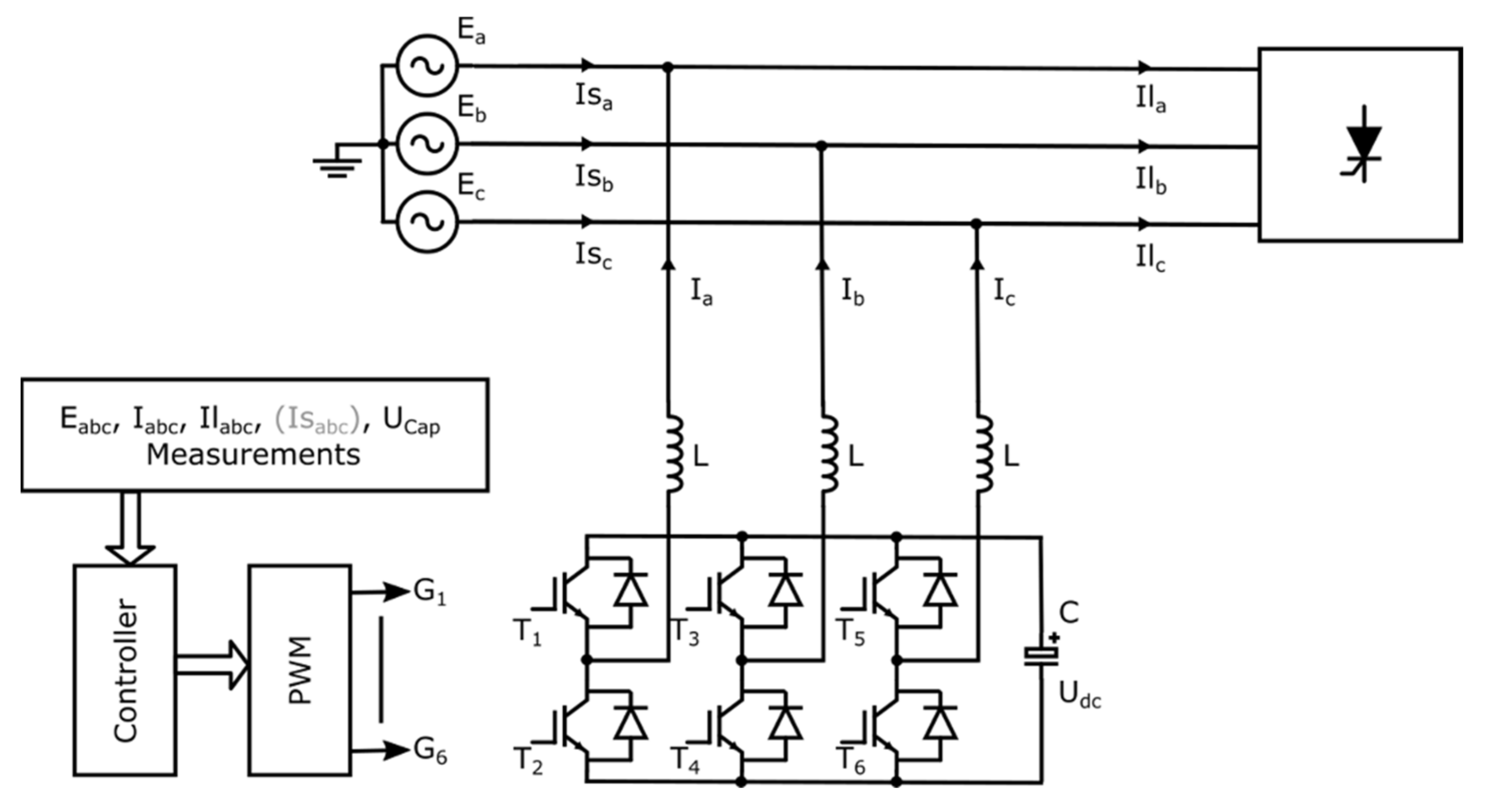
Figure 1 shows a block diagram of the three-phase, three-wire S-APF system studied. As a non-linear load, a thyristor rectifier with resistance load at the DC side has been used. The S-APF configuration is based on a voltage source inverter connected to a capacitor at the DC side. The reduction in unwanted load currents Il_abc components is obtained by injecting equal but reverse sign compensating currents I_abc, which are produced by S-APF in accordance with the control algorithms. The shape of the compensating currents is fully controlled by the S-APF and finally determines the shape of the grid currents Is_abc.

2.2. Modeling of the Inverter

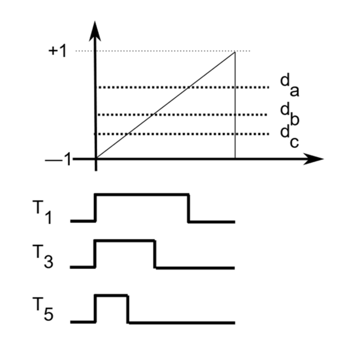
The T₁, T₂, T₃, T₄, T₅, and T₆ switches are controlled by three pairs of complementary PWM signals. The T₁, T₃, and T₅ signals are inverted to the signals T₂, T₄, and T₆, respectively. Control signals d_a, d_b, and d_c vary from −1.0 to +1.0. They are compared to the sawtooth carrier and applied to the generation of PWM waves, as shown in Figure 2.

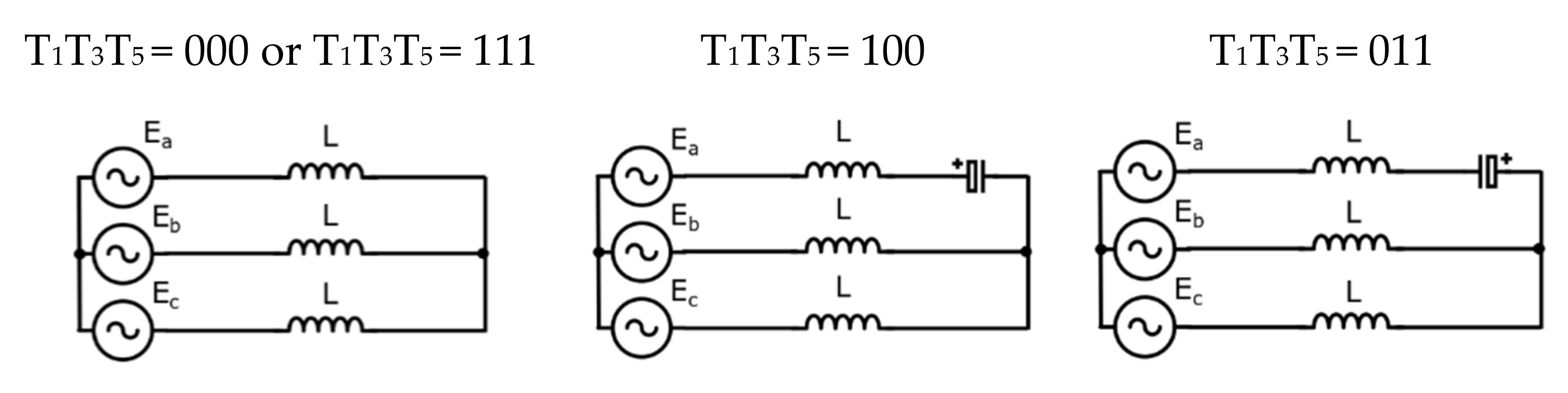
Figure 3 presents the equivalent configurations of the inverter for the first phase for the respective states of the T₁, T₃, and T₅ switches. From the figures, one can derive the equation for the first phase inverter current, and by analogy, the remaining two currents can also be given.

Considering inductance L of the S-APF, the equations of the currents at the end of the switching period are as follows:

$$I\left(t+T_0\right)=\left[\begin{array}{c}{I}_a+\frac{T_0}{3L}\left(-2E_a+E_b+E_c-U_{\mathrm{dc}}\left(-2d_a+d_b+d_c\right)\right)\\ I_b+\frac{T_0}{3L}\left(E_a-2E_b+E_c-U_{\mathrm{dc}}\left(d_a-2d_b+d_c\right)\right)\\ I_c+\frac{T_0}{3L}\left(E_a+E_b-2E_c-U_{\mathrm{dc}}\left(d_a+d_b-2d_c\right)\right)\end{array}\right], I_a+I_b+I_c=0$$

(1)

where:

$d_a, d_b, d_c$—are control signals applied to generate the PWM waves.

$E_a, E_b, E_c$—are the grid voltages.

$I_a, I_b, I_c$—are the output inverter currents at the beginning of a switching period.

$T_0$—is the switching period.

$U_{\mathrm{dc}}$—is the DC voltage.

The aim of the inverter is to follow the reference currents (2) calculated by the controller of the S-APF.

$$I_{ref}=\left[\begin{array}{c}{I}_{refa}\\ I_{refb}\\ I_{refc}\end{array}\right],\hspace{1em}{I}_{refa}+I_{refb}+I_{refc}=0$$

(2)

The control vector

$$d=\left[\begin{array}{c}{d}_a\\ d_b\\ d_c\end{array}\right],\hspace{1em}-1.0\le d\le +1.0$$

(3)

determines the behavior of the controller. The quality of the controller can be defined quantitatively as the distance between the reference and filter currents:

$$f\left(d\right)=\parallel I_{ref}-I\left(t+T_0\right)\parallel ={\left(I_{ref}-I\left(t+T_0\right)\right)}^T\left(I_{ref}-I\left(t+T_0\right)\right)$$

(4)

3. The KKT Algorithm

3.1. Calculation Algorithm for the Optimal Control

The current controller solves the following optimization problem:

$$\begin{gathered} \underset{d}{\min }f\left(d\right), \\ {g}_i\left(d\right)\le 0,\hspace{1em}i=1..6 , \end{gathered}$$

(5)

where vector $g_i\left(d\right)$ defines the constraints of the control signal:

$$g_i\left(d\right)={\left[\begin{array}{c}{d}_a-1\\ -d_a-1\\ d_b-1\\ -d_b-1\\ d_c-1\\ -d_c-1\end{array}\right]}^T\le 0.$$

(6)

By applying the KKT conditions to (5) and (6), the following conditions for the optimal solution d* can be formulated:

$$\left\{\begin{array}{c}\nabla f\left(d^{*}\right)+{{\displaystyle \sum }}_{i=1}^6{\mu }_i\nabla g_i\left(d^{*}\right)=0\\ {\mu }_i{g}_i\left(d^{*}\right)=0\\ {\mu }_i\ge 0\\ g_i\left(d^{*}\right)\le 0\end{array}\right.,\hspace{1em}i=\mathrm{1..6}.$$

(7)

where:

${\mu }_i$—Lagrange multipliers;

$\nabla f$—gradient of the f function;

$\nabla g_i$—g_i gradient.

The gradients of f and $g_i$ functions can be calculated from (1), (4), and (6):

$$\nabla f\left(d\right)=\left[\begin{array}{c}\frac{2T_0{U}_{\mathrm{dc}}\left(2I_{a}L-I_{b}L-I_{c}L-2I_{\mathrm{refa}}L+I_{\mathrm{refb}}L+I_{\mathrm{refc}}L-2E_a{T}_0+E_b{T}_0+E_c{T}_0+2T_0{U}_{\mathrm{dc}}{d}_a-T_0{U}_{\mathrm{dc}}{d}_b-T_0{U}_{\mathrm{dc}}{d}_c\right)}{3L^2}\\ -\frac{2T_0{U}_{\mathrm{dc}}\left(I_{a}L-2I_{b}L+I_{c}L-I_{\mathrm{refa}}L+2I_{\mathrm{refb}}L-I_{\mathrm{refc}}L-E_a{T}_0+2E_b{T}_0-E_c{T}_0+T_0{U}_{\mathrm{dc}}{d}_a-2T_0{U}_{\mathrm{dc}}{d}_b+T_0{U}_{\mathrm{dc}}{d}_c\right)}{3L^2}\\ -\frac{2T_0{U}_{\mathrm{dc}}\left(I_{a}L+I_{b}L-2I_{c}L-I_{\mathrm{refa}}L-I_{\mathrm{refb}}L+2I_{\mathrm{refc}}L-E_a{T}_0-E_b{T}_0+2E_c{T}_0+T_0{U}_{\mathrm{dc}}{d}_a+T_0{U}_{\mathrm{dc}}{d}_b-2T_0{U}_{\mathrm{dc}}{d}_c\right)}{3L^2}\end{array}\right],$$

(8)

$$\nabla g_i\left(d\right)=\left[\begin{array}{cccccc}1& -1& 0& 0& 0& 0\\ 0& 0& 1& -1& 0& 0\\ 0& 0& 0& 0& 1& -1\end{array}\right].$$

(9)

The constraints (6) create a box; thus, for the convex function (4) there exist twenty-seven possible locations of the optimal solution: a single location inside the box, six locations at the planes, twelve at the edges, and eight at the corners. Solving the first two equations of (7) gives the following solutions:

$$d_a=\left[\begin{array}{c}1\\ -1\\ 1\\ -1\\ \frac{T_0{U}_{\mathrm{dc}}-I_{a}L+I_{b}L+I_{\mathrm{refa}}L-I_{\mathrm{refb}}L+E_a{T}_0-E_b{T}_0}{T_0{U}_{\mathrm{dc}}}\\ -\frac{T_0{U}_{\mathrm{dc}}+I_{a}L-I_{b}L-I_{\mathrm{refa}}L+I_{\mathrm{refb}}L-E_a{T}_0+E_b{T}_0}{T_0{U}_{\mathrm{dc}}}\\ -1\\ 1\\ -1\\ 1\\ -\frac{2I_{a}L-I_{b}L-I_{c}L-2I_{\mathrm{refa}}L+I_{\mathrm{refb}}L+I_{\mathrm{refc}}L-2E_a{T}_0+E_b{T}_0+E_c{T}_0}{2T_0{U}_{\mathrm{dc}}}\\ -\frac{2I_{a}L-I_{b}L-I_{c}L-2I_{\mathrm{refa}}L+I_{\mathrm{refb}}L+I_{\mathrm{refc}}L-2E_a{T}_0+E_b{T}_0+E_c{T}_0}{2T_0{U}_{\mathrm{dc}}}\\ -\frac{I_{a}L-I_{c}L-I_{\mathrm{refa}}L+I_{\mathrm{refc}}L-E_a{T}_0\mathrm{+}{E}_c{T}_0}{T_0{U}_{\mathrm{dc}}}\\ 1\\ -1\\ 1\\ -1\\ -1\\ 1\\ \frac{T_0{U}_{\mathrm{dc}}-I_{a}L+I_{c}L+I_{\mathrm{refa}}L-I_{\mathrm{refc}}L+E_a{T}_0-E_c{T}_0}{T_0{U}_{\mathrm{dc}}}\\ -\frac{T_0{U}_{\mathrm{dc}}+I_{a}L-I_{c}L-I_{\mathrm{refa}}L+I_{\mathrm{refc}}L-E_a{T}_0+E_c{T}_0}{T_0{U}_{\mathrm{dc}}}\\ 1\\ -1\\ 1\\ -1\\ \frac{2T_0{U}_{\mathrm{dc}}-2I_{a}L+I_{b}L+I_{c}L+2I_{\mathrm{refa}}L-I_{\mathrm{refb}}L-I_{c}L+2E_a{T}_0-E_b{T}_0-E_c{T}_0}{2T_0{U}_{\mathrm{dc}}}\\ -\frac{2T_0{U}_{\mathrm{dc}}+2I_{a}L-I_{b}L-I_{c}L-2I_{\mathrm{refa}}L+I_{\mathrm{refb}}L+I_{c}L-2E_a{T}_0+E_b{T}_0+E_c{T}_0}{2T_0{U}_{\mathrm{dc}}}\end{array}\right],$$

(10)

$$d_b=\left[\begin{array}{c}1\\ -1\\ \frac{T_0{U}_{\mathrm{dc}}+I_{a}L-I_{b}L-I_{\mathrm{refa}}L+I_{\mathrm{refb}}L-E_a{T}_0+E_b{T}_0}{T_0{U}_{\mathrm{dc}}}\\ -\frac{T_0{U}_{\mathrm{dc}}-I_{a}L+I_{b}L+I_{\mathrm{refa}}L-I_{\mathrm{refb}}L+E_a{T}_0-E_b{T}_0}{T_0{U}_{\mathrm{dc}}}\\ 1\\ -1\\ 1\\ -1\\ -\frac{2I_{b}L-I_{a}L-I_{c}L+I_{\mathrm{refa}}L-2I_{\mathrm{refb}}L+I_{\mathrm{refc}}L+E_a{T}_0-2E_b{T}_0+E_c{T}_0}{2T_0{U}_{\mathrm{dc}}}\\ -\frac{2I_{b}L-I_{a}L-I_{c}L+I_{\mathrm{refa}}L-2I_{\mathrm{refb}}L+I_{\mathrm{refc}}L+E_a{T}_0-2E_b{T}_0+E_c{T}_0}{2T_0{U}_{\mathrm{dc}}}\\ -1\\ 1\\ -\frac{I_{b}L-I_{C}L-I_{\mathrm{refb}}L+I_{\mathrm{refc}}L-E_b{T}_0+E_c{T}_0}{T_0{U}_{\mathrm{dc}}}\\ 1\\ 1\\ -1\\ -1\\ 1\\ -1\\ \frac{T_0{U}_{\mathrm{dc}}-I_{b}L+I_{c}L+I_{\mathrm{refb}}L-I_{\mathrm{refc}}L+E_b{T}_0-E_c{T}_0}{T_0{U}_{\mathrm{dc}}}\\ -\frac{T_0{U}_{\mathrm{dc}}+I_{b}L-I_{c}L-I_{\mathrm{refb}}L+I_{\mathrm{refc}}L-E_b{T}_0+E_c{T}_0}{T_0{U}_{\mathrm{dc}}}\\ 1\\ -1\\ \frac{2T_0{U}_{\mathrm{dc}}+I_{a}L-2I_{b}L+I_{c}L-I_{\mathrm{refa}}L+2I_{\mathrm{refb}}L-I_{\mathrm{refc}}L-E_a{T}_0+2E_b{T}_0-E_c{T}_0}{2T_0{U}_{\mathrm{dc}}}\\ -\frac{2T_0{U}_{\mathrm{dc}}-I_{a}L+2I_{b}L-I_{c}L+I_{\mathrm{refa}}L-2I_{\mathrm{refb}}L+I_{\mathrm{refc}}L+E_a{T}_0-2E_b{T}_0+E_c{T}_0}{2T_0{U}_{\mathrm{dc}}}\\ 1\\ -1\end{array}\right],$$

(11)

$$d_c=\left[\begin{array}{c}1\\ -1\\ \frac{T_0{U}_{\mathrm{dc}}+I_{a}L-I_{c}L-I_{\mathrm{refa}}L+I_{\mathrm{refc}}L-E_a{T}_0+E_c{T}_0}{T_0{U}_{\mathrm{dc}}}\\ -\frac{T_0{U}_{\mathrm{dc}}-I_{a}L+I_{c}L+I_{\mathrm{refa}}L-I_{\mathrm{refc}}L+E_a{T}_0-E_c{T}_0}{T_0{U}_{\mathrm{dc}}}\\ \frac{T_0{U}_{\mathrm{dc}}+I_{b}L-I_{c}L-I_{\mathrm{refb}}L+I_{\mathrm{refc}}L-E_b{T}_0+E_c{T}_0}{T_0{U}_{\mathrm{dc}}}\\ -\frac{T_0{U}_{\mathrm{dc}}-I_{b}L+I_{c}L+I_{\mathrm{refb}}L-I_{\mathrm{refc}}L+E_b{T}_0+E_c{T}_0}{T_0{U}_{\mathrm{dc}}}\\ \frac{3T_0{U}_{\mathrm{dc}}-I_{a}L+2I_{b}L-I_{c}L+I_{\mathrm{refa}}L-2I_{\mathrm{refb}}L+I_{\mathrm{refc}}L+E_a{T}_0-2E_b{T}_0+E_c{T}_0}{T_0{U}_{\mathrm{dc}}}\\ -\frac{3T_0{U}_{\mathrm{dc}}+I_{a}L-2I_{b}L+I_{c}L-I_{\mathrm{refa}}L+2I_{\mathrm{refb}}L-I_{\mathrm{refc}}L-E_a{T}_0+2E_b{T}_0-E_c{T}_0}{T_0{U}_{\mathrm{dc}}}\\ 1\\ -1\\ 1\\ -1\\ 0\\ -1\\ 1\\ 1\\ 1\\ -1\\ -1\\ 1\\ -1\\ \frac{T_0{U}_{\mathrm{dc}}-I_{a}L+2I_{b}L-I_{c}L+I_{\mathrm{refa}}L-2I_{\mathrm{refb}}L+I_{\mathrm{refc}}L+E_a{T}_0-2E_b{T}_0+E_c{T}_0}{T_0{U}_{\mathrm{dc}}}\\ -\frac{T_0{U}_{\mathrm{dc}}+I_{a}L-2I_{b}L+I_{c}L-I_{\mathrm{refa}}L+2I_{\mathrm{refb}}L-I_{\mathrm{refc}}L-E_a{T}_0+2E_b{T}_0-E_c{T}_0}{T_0{U}_{\mathrm{dc}}}\\ 1\\ -1\\ 1\\ -1\end{array}\right],$$

(12)

The complexity of the solutions for six ${\mu }_i$ multipliers is similar to (10)–(12); therefore, considering the time required to perform the calculations, the calculations of ${\mu }_i$ and the checking of the inequality conditions in (7) to obtain the optimal solution are omitted. Alternatively, the following algorithm for finding the optimal solution is proposed:

• From Equations (10)–(12), calculate twenty-seven candidates for the optimal solution.
• From the list of candidates, remove the solutions which violate the constraints (6).
• For the remaining elements, use Equation (1) to calculate the current; next, calculate the values of the penalty function (4).
• Select for optimal control $d^{*}$, which is the element with minimum value of the penalty function (4).

3.2. Simplification of the Algorithm

The presented optimal control calculation algorithm must be calculated in real-time by the APF controller. As formulas (10)–(12) require a significant amount of calculations, it is essential to try and simplify the algorithm to reduce the computation time.

One can notice that, according to Equation (1), adding a constant value to all control signals (d_a, d_b, and d_c) does not change the value of the I(t + T₀) current. Of course, the control values have to meet the constraints. This means that by shifting the control values, the smallest control can always have the value −1.0 or the greatest control value +1.0.

Let us assume that, from the three control signals, the d_a is minimal, so it can be fixed to the value −1.0. Equations (1) and (3) can be reformulated as:

$$I\left(t+T_0\right)=\left[\begin{array}{c}{I}_a+\frac{T_0}{3L}\left(-2E_a+E_b+E_c-U_{\mathrm{dc}}\left(2.0+d_b+d_c\right)\right)\\ I_b+\frac{T_0}{3L}\left(E_a-2E_b+E_c-U_{\mathrm{dc}}\left(-1.0-2d_b+d_c\right)\right)\\ I_c+\frac{T_0}{3L}\left(E_a+E-2E_c-U_{\mathrm{dc}}\left(-1.0+d_b-2d_c\right)\right)\end{array}\right],$$

(13)

$$d=\left[\begin{array}{c}{d}_b\\ d_c\end{array}\right],-1.0\le d\le +1.0.$$

(14)

The new optimization problem can be stated as:

$$\begin{gathered} \underset{d}{\min }f\left(d\right), \\ {g}_i\left(d\right)\le 0;i=1\dots 4, \end{gathered}$$

(15)

$$g_i\left(d\right)={\left[\begin{array}{c}{d}_b-1\\ -d_b-1\\ d_c-1\\ -d_c-1\end{array}\right]}^T\le 0,$$

(16)

and the new KKT conditions are:

$$\left\{\begin{array}{c}\nabla f\left(d^{*}\right)+{\displaystyle {\displaystyle \sum }_{i=1}^4}{\mu }_i\nabla g_i\left(d^{*}\right)=0\\ {\mu }_i{g}_i\left(d^{*}\right)=0\\ {\mu }_i\ge 0\\ g_i\left(d^{*}\right)\le 0\end{array}\right.,\hspace{1em}i=1\dots 4.$$

(17)

The respective gradients are as follows:

$$\nabla f\left(d\right)=\left[\begin{array}{c}\frac{2T_0{U}_{\mathrm{dc}}\left(T_0{U}_{\mathrm{dc}}-I_{a}L+2I_{b}L-I_{c}L-3I_{\mathrm{refb}}L+E_a{T}_0-2E_b{T}_0+E_c{T}_0+2T_0{U}_{\mathrm{dc}}{d}_b-T_0{U}_{\mathrm{dc}}{d}_c\right)}{3L^2}\\ \frac{2T_0{U}_{\mathrm{dc}}\left(T_0{U}_{\mathrm{dc}}-I_{a}L-I_{b}L+2I_{c}L-3I_{\mathrm{refc}}L+E_a{T}_0+E_b{T}_0-2E_c{T}_0-T_0{U}_{\mathrm{dc}}{d}_b+2T_0{U}_{\mathrm{dc}}{d}_c\right)}{3L^2}\end{array}\right]$$

(18)

$$\nabla g_i\left(d\right)=\left[\begin{array}{cccc}1& -1& 0& 0\\ 0& 0& 1& -1\end{array}\right].$$

(19)

The solution of the first two equations of (17) gives the set of possible optimal solutions. Taking into account that d_a = −1.0, nine possible solutions are given as follows:

$$d=\left[\begin{array}{ccc}-1& -1& -1\\ -1& \frac{I_{a}L-T_0{U}_{\mathrm{dc}}-I_{b}L+2I_{\mathrm{refb}}L+I_{\mathrm{refc}}L-E_a{T}_0+E_b{T}_0}{T_0{U}_{\mathrm{dc}}}& \frac{I_{a}L-T_0{U}_{\mathrm{dc}}-I_{c}L+I_{\mathrm{refb}}L+2I_{\mathrm{refc}}L-E_a{T}_0+E_c{T}_0}{T_0{U}_{\mathrm{dc}}}\\ -1& 1& \frac{I_{a}L+I_{b}L-2I_{c}L+3I_{\mathrm{refc}}L-E_a{T}_0-E_b{T}_0+2E_c{T}_0}{2T_0{U}_{\mathrm{dc}}}\\ -1& \frac{I_{a}L-2I_{b}L+I_{c}L+3I_{\mathrm{refb}}L-E_a{T}_0+2E_b{T}_0-E_c{T}_0}{2T_0{U}_{\mathrm{dc}}}& 1\\ -1& -1& -\frac{2T_0{U}_{\mathrm{dc}}-I_{a}L-I_{b}L+2I_{c}L-3I_{\mathrm{refc}}L+E_a{T}_0+E_b{T}_0-2E_c{T}_0}{2T_0{U}_{\mathrm{dc}}}\\ -1& -\frac{2T_0{U}_{\mathrm{dc}}-I_{a}L+2I_{b}L-I_{c}L-3I_{\mathrm{refb}}L+E_a{T}_0-2E_b{T}_0+E_c{T}_0}{2T_0{U}_{\mathrm{dc}}}& -1\\ -1& 1& 1\\ -1& -1& 1\\ -1& 1& -1\end{array}\right].$$

(20)

The same steps can be repeated for the assumption that d_b and d_c are minimal. In these cases, the possible optimal sets of control signals are as follows:

$$d=\left[\begin{array}{ccc}-1& -1& -1\\ \frac{I_{b}L-I_{a}L-T_0{U}_{\mathrm{dc}}+2I_{\mathrm{refa}}L+I_{\mathrm{refc}}L+E_a{T}_0-E_b{T}_0}{T_0{U}_{\mathrm{dc}}}& -1& \frac{I_{b}L-T_0{U}_{\mathrm{dc}}-I_{c}L+I_{\mathrm{refa}}L+2I_{\mathrm{refc}}L-E_b{T}_0+E_c{T}_0}{T_0{U}_{\mathrm{dc}}}\\ 1& -1& \frac{I_{a}L+I_{b}L-2I_{c}L+3I_{\mathrm{refc}}L-E_a{T}_0-E_b{T}_0+2E_c{T}_0}{2T_0{U}_{\mathrm{dc}}}\\ \frac{I_{b}L-2I_{a}L+I_{c}L+3I_{\mathrm{refa}}L+2E_a{T}_0-E_b{T}_0-E_c{T}_0}{2T_0{U}_{\mathrm{dc}}}& -1& 1\\ -1& -1& -\frac{2T_0{U}_{\mathrm{dc}}-I_{a}L-I_{b}L+2I_{c}L-3I_{\mathrm{refc}}L+E_a{T}_0+E_b{T}_0-2E_c{T}_0}{2T_0{U}_{\mathrm{dc}}}\\ -\frac{2T_0{U}_{\mathrm{dc}}+2I_{a}L-I_{b}L-I_{c}L-3I_{\mathrm{refa}}L-2E_a{T}_0+E_b{T}_0+E_c{T}_0}{2T_0{U}_{\mathrm{dc}}}& -1& -1\\ 1& -1& 1\\ -1& -1& 1\\ 1& -1& -1\end{array}\right],$$

(21)

$$d=\left[\begin{array}{ccc}-1& -1& -1\\ \frac{I_{c}L-I_{a}L-T_0{U}_{\mathrm{dc}}+2I_{\mathrm{refa}}L+I_{\mathrm{refb}}L+E_a{T}_0-E_c{T}_0}{T_0{U}_{\mathrm{dc}}}& \frac{I_{c}L-I_{b}L-T_0{U}_{\mathrm{dc}}+I_{\mathrm{refa}}L+2I_{\mathrm{refb}}L+E_b{T}_0-E_c{T}_0}{T_0{U}_{\mathrm{dc}}}& -1\\ 1& \frac{I_{a}L-2I_{b}L+I_{c}L+3I_{\mathrm{refb}}L-E_a{T}_0+2E_b{T}_0-E_c{T}_0}{2T_0{U}_{\mathrm{dc}}}& -1\\ \frac{I_{b}L-2I_{a}L+I_{c}L+3I_{\mathrm{refa}}L+2E_a{T}_0-E_b{T}_0-E_c{T}_0}{2T_0{U}_{\mathrm{dc}}}& 1& -1\\ -1& -\frac{2T_0{U}_{\mathrm{dc}}-I_{a}L+2I_{b}L-I_{c}L-3I_{\mathrm{refb}}L+E_a{T}_0-2E_b{T}_0+E_c{T}_0}{2T_0{U}_{\mathrm{dc}}}& -1\\ -\frac{2T_0{U}_{\mathrm{dc}}+2I_{a}L-I_{b}L-I_{c}L-3I_{\mathrm{refa}}L-2E_a{T}_0+E_b{T}_0+E_c{T}_0}{2T_0{U}_{\mathrm{dc}}}& -1& -1\\ 1& 1& -1\\ -1& 1& -1\\ 1& -1& -1\end{array}\right].$$

(22)

Like Equations (10)–(12), Equations (20)–(22) define twenty-seven control vectors, one of which has to be an optimal control. However, one can notice that:

• Equations (10)–(12) contain twenty-six non-constant elements, while Equations (20)–(22) include only eighteen elements which have to be calculated.
• In Equations (20)–(22), five rows are duplicated, so only twenty-two control vectors have to be checked to find the optimal one.

The simplified version of the algorithm works almost identically to the version presented in the previous chapter; the only difference is the use of Equations (20)–(22) instead of Equations (10)–(12) to find the optimal solution. The limited number of tested control vectors and the reduced computation complexity only reduce computation time, facilitating the implementation of the algorithm in real-time.

3.3. Proposed Control System Implementation Method

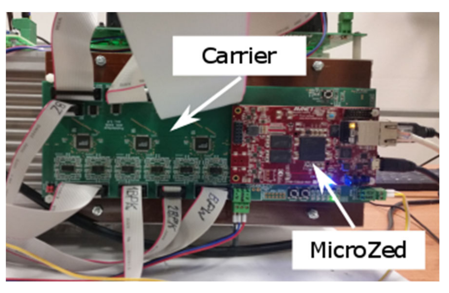
The APF controller runs on a MicroZed board [26]. The MicroZed is plugged into the carrier board containing A/D converters and an interface to the IGBT drivers (see Figure 4).

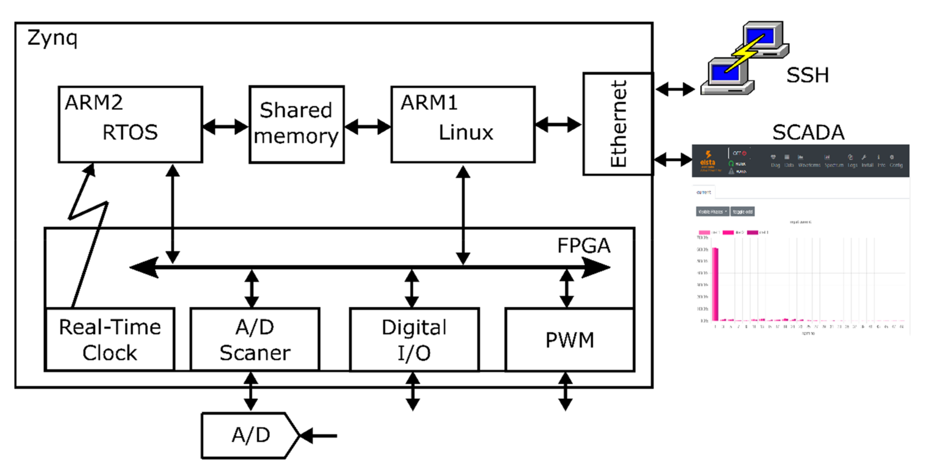
MicroZed contains an integrated circuit, Xilinx Zynq, which includes two ARM Cortex A9 processors and a reconfigurable FPGA fabric. The task of the S-APF controller has been divided between both the processors and FPGA (Figure 5):

• The first ARM processor runs the Linux operating system. It runs all non-real-time tasks, such as RTOS supervision, tuning parameters, network services (FTP, HTTP), on-line monitoring and communication with a user, and SCADA systems.
• The second ARM processor runs the FreeRTOS real-time operating system. Both processors communicate via a shared memory buffer. It performs time-critical tasks, e.g., controlling the A/D converters to read the values of voltages and currents, calculating the control values, and setting the duty cycle of the output PWM blocks. It also performs tasks related to ensuring the safe operation of the APF and supervises the sequences of safe start and termination of the S-APF operation. Most of these tasks are performed with a sampling frequency of 14.629 kHz, providing 2048 samples per 7 grid periods. The sampling frequency determines a maximum period of approximately 68 µs during which all calculations have to be performed, including the calculation of the optimal control vector presented in this paper.

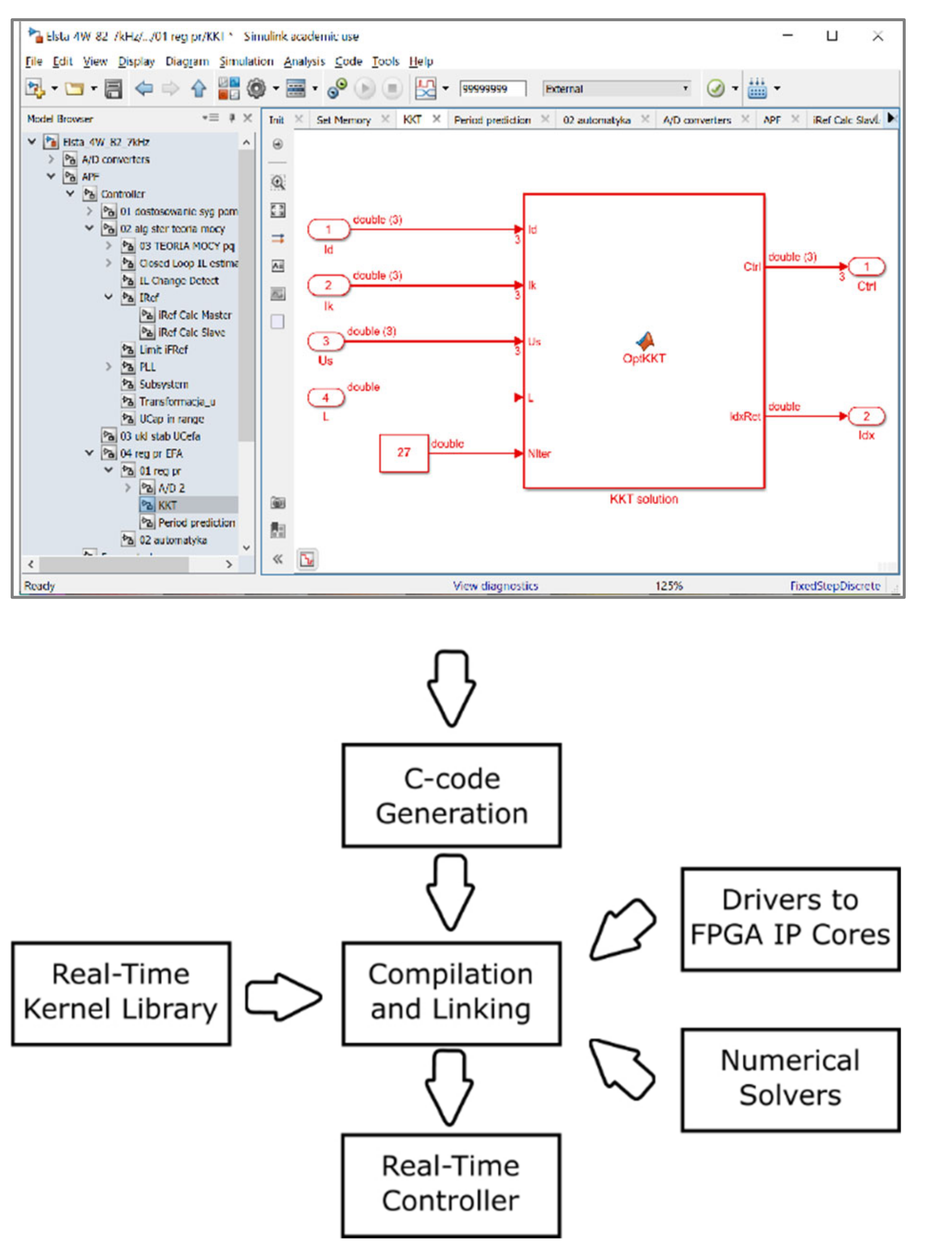
The implementation of the S-APF controller was made according to the Model-Based Design (MBD) principle. The MBD focuses on the modelling and validation of a model by simulation while the implementation details are hidden and performed automatically [27,28,29]. The design and simulation stages are conducted in Simulink and after the validation of the model, the C-code of the real-time controller, which is functionally equivalent to the model, is automatically generated.

Due to the high sampling rate of 14.629 kHz, FreeRTOS was used as a real-time operating system to guarantee the accuracy of the calculations. Equations (20)–(22), along with the algorithm for finding the optimal control vector, have been implemented in the “KKT solution” block (Figure 6). The generated code with real-time kernel files is automatically compiled and an application is created that performs calculations every 68 ms.

Besides the execution of the algorithm for finding the optimal control vector, the real-time application performs other functions related to S-APF control, e.g., the reading of voltages and currents from ADC converters, implementation of the PLL algorithm synchronizing the S-APF to the grid, calculation of the reference currents in the control algorithm module, and communication with output PWM blocks and functions monitoring safe S-APF operation. The algorithm is executed on the ARM A9 processor working with a 667 MHz clock. The execution time of the algorithm is about 45 ms, of which the discussed algorithm for finding the optimal control vector calculates about 13 ms.

4. Experimental Results

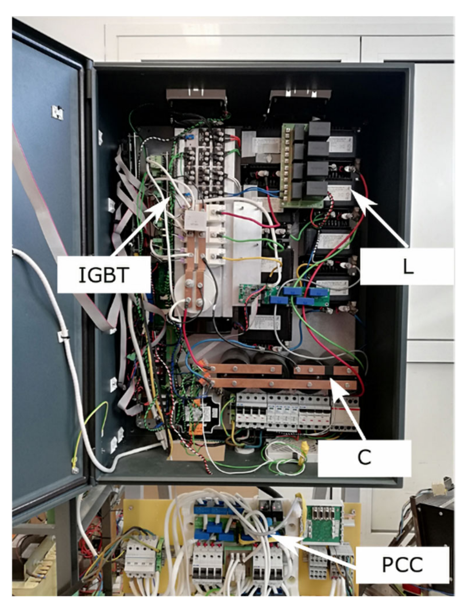
The algorithm was verified on a laboratory stand with a 30 kVA three-phase three-wire S-APF (Figure 7). The basic parameters of the test system: supply voltages U_abc 3 × 400/230 V, fundamental harmonic f₍₁₎ = 50 Hz, choke inductance at the AC side of S-APF: L = 2 mH, capacitor capacitance at the DC side of S-APF: C = 6.6 mF, reference voltage in the DC circuit U_dc,ref = 800 V, switching frequency of IGBT transistors f_sw = 14.6 kHz.

To verify the quality of the presented algorithm, its operation with the classical PI algorithm was compared. Two series of experiments were performed for the identical non-linear load, one for the PI algorithm and the other for the presented algorithm for finding optimal controls. In both cases, the accuracy of following the reference current values was applied as a quality criterion, defined by Equation (23).

$$J={\displaystyle \sum _{i=1}^n}\sqrt{(I_a-I_{\mathit{refa}}{)}^2+(I_b-I_{\mathit{refb}}{)}^2+(I_c-I_{\mathit{refc}}{)}^2}$$

(23)

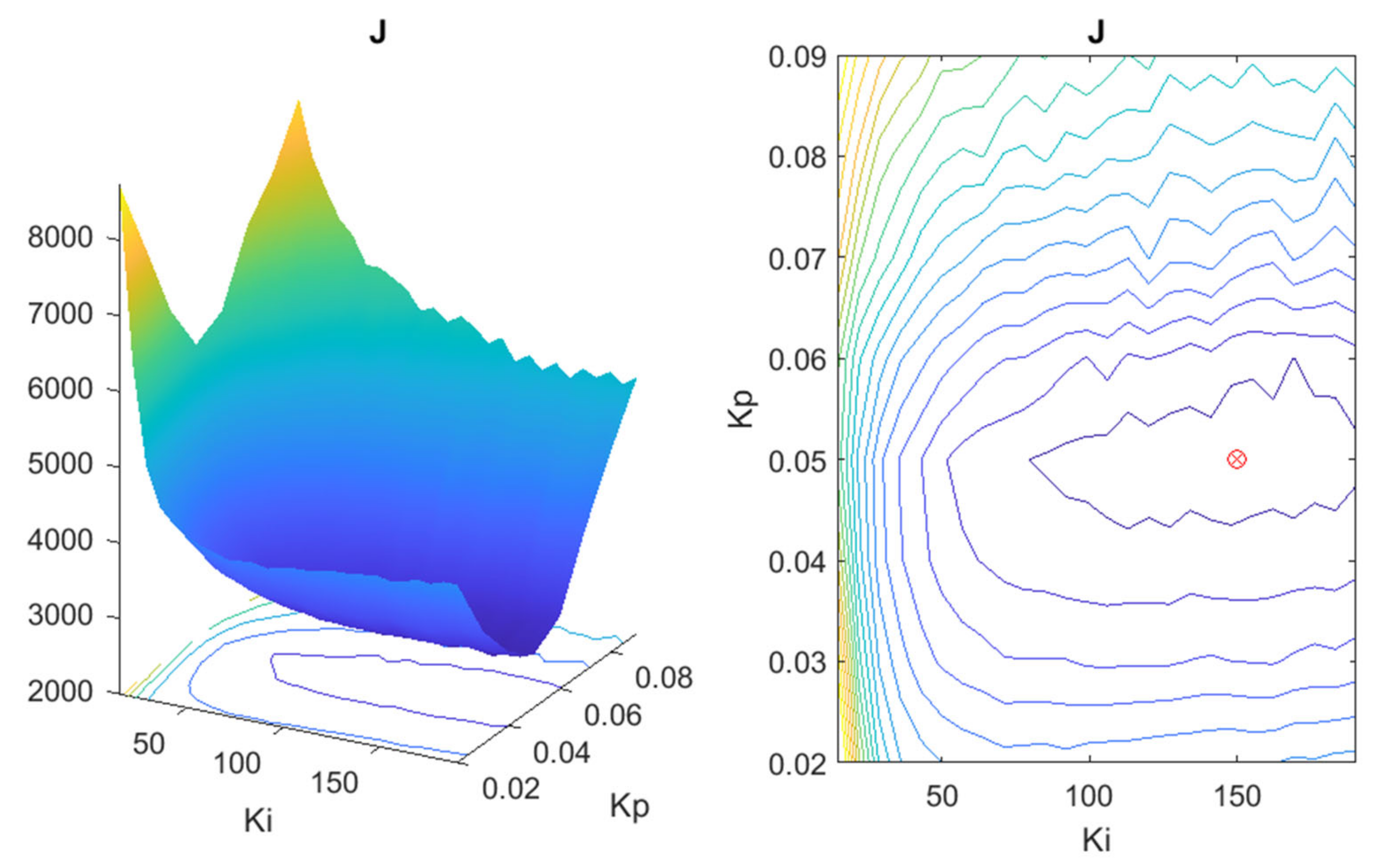
In the case of the PI controller, the value of criterion (23) depends on the settings of the K_p and K_i parameters. The parameter values optimizing the cost function (23) were obtained by scanning the values in the neighborhood of the presumed optimal values for the PI controller. Scanning was performed during the S-APF operation. The values of the criterion function for different pairs of parameter values K_p and K_i are shown in Figure 8. The optimal parameters of the PI controller obtained in the sense of criterion (23) are K_p = 150 and K_i = 0.05.

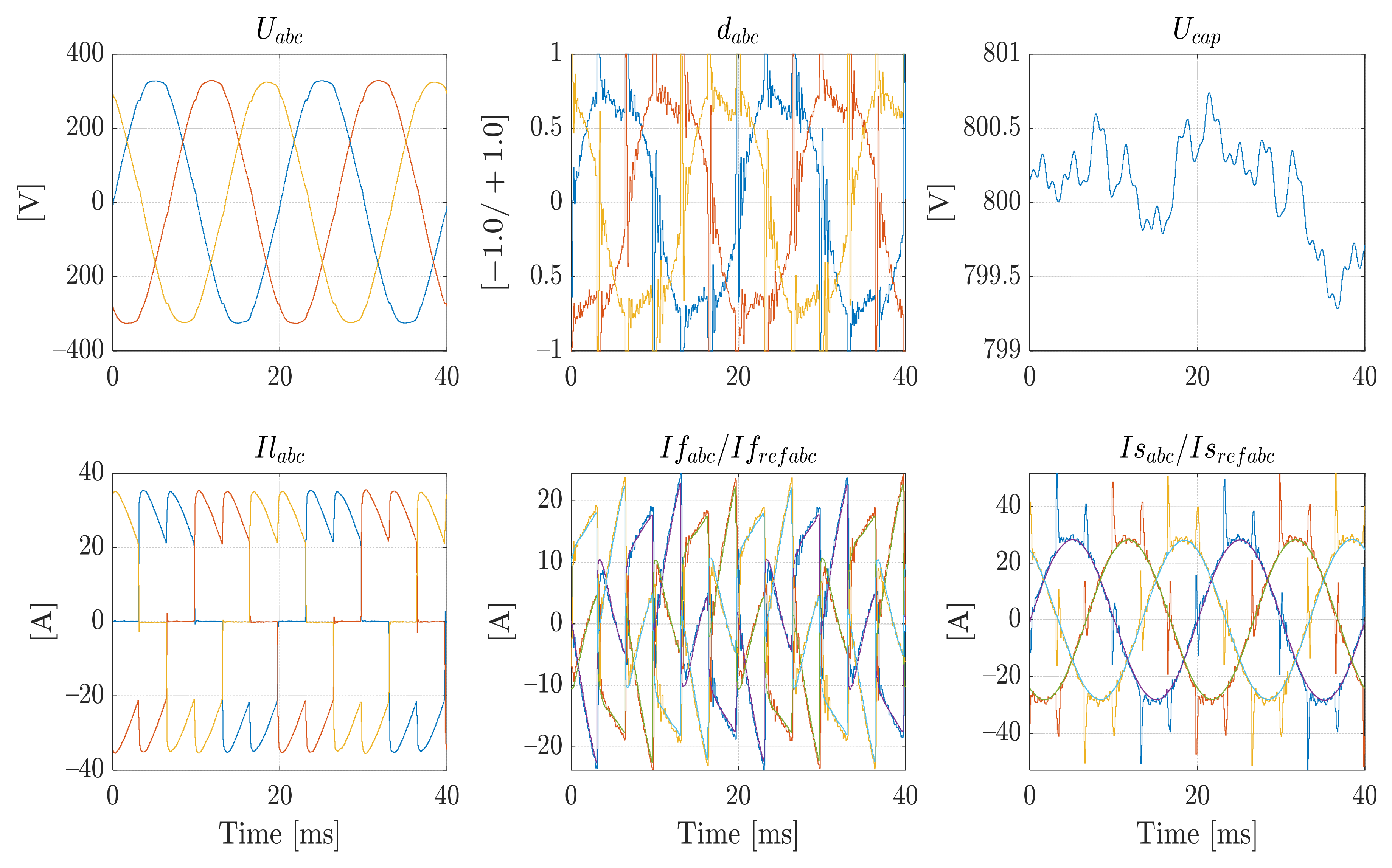
An example of load compensation controlled by the PI is shown in Figure 9. Grid voltages U_abc = E_abc, load currents Il_abc, reference filter currents If_refabc, filter output currents If_abc = I_abc, and reference and real grid currents Is_abc, Is_refabc = Il_abc − If_refabc, respectively, are presented. Additionally, the value of the DC circuit voltage U_cap = U_dc and the output from the PI controller d_abc are presented. The THD factor of the load current is 33%. The filter operation reduces the THD of the grid currents to a level of 19.5%.

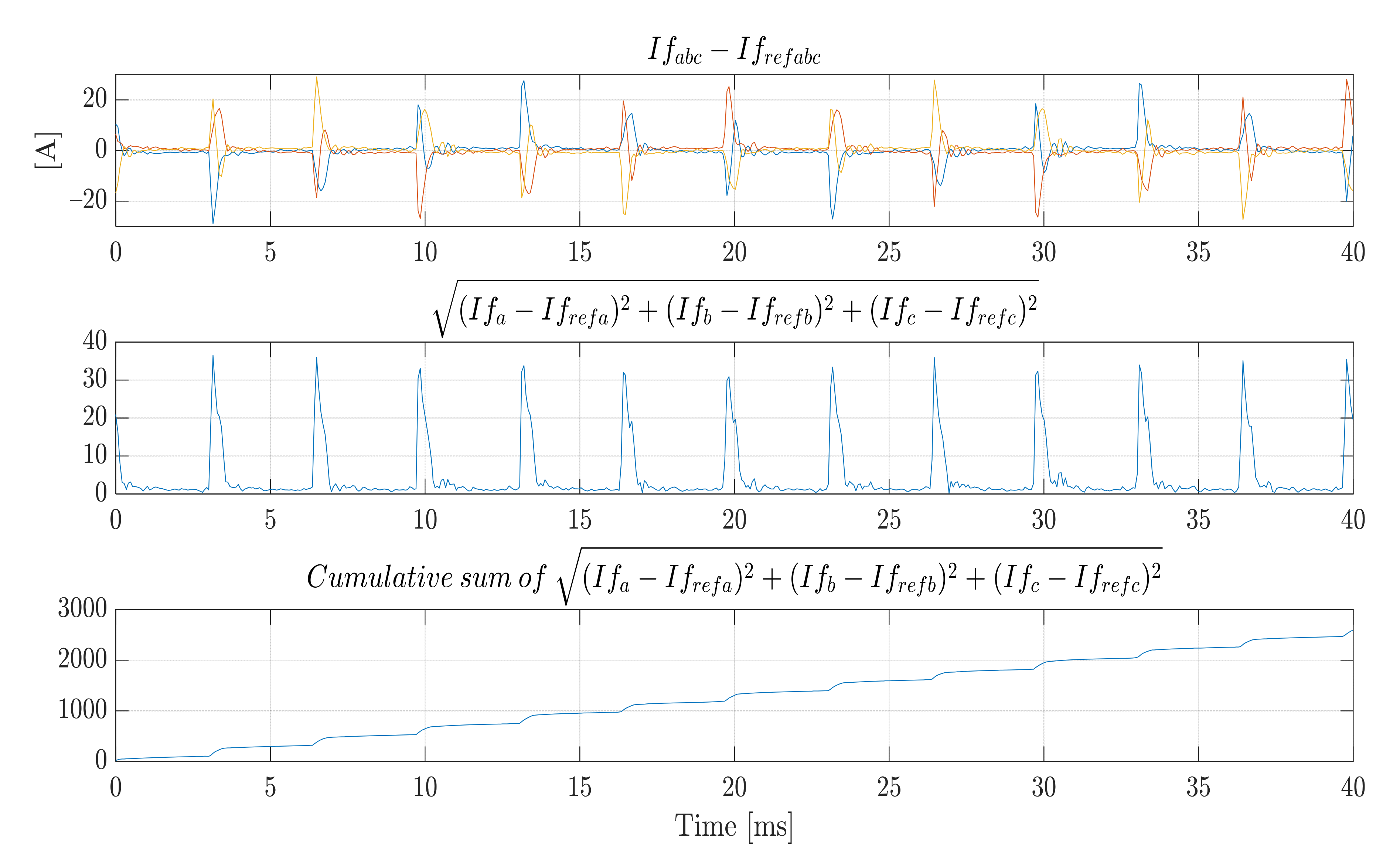
Figure 10 shows the regulation error as the difference between the reference and actual filter current. In the presented time horizon, the cumulative control error (23) is equal to approximately 2600. One can notice that the commutation changes in the load current have the greatest impact on the error. The PI controller saturates in these cases, going into a state that can be interpreted as a lack of feedback. It results in a high THD grid current level due to a lack of good compensation of rapid commutation changes in the load currents, which is a characteristic state of operation of power electronic systems.

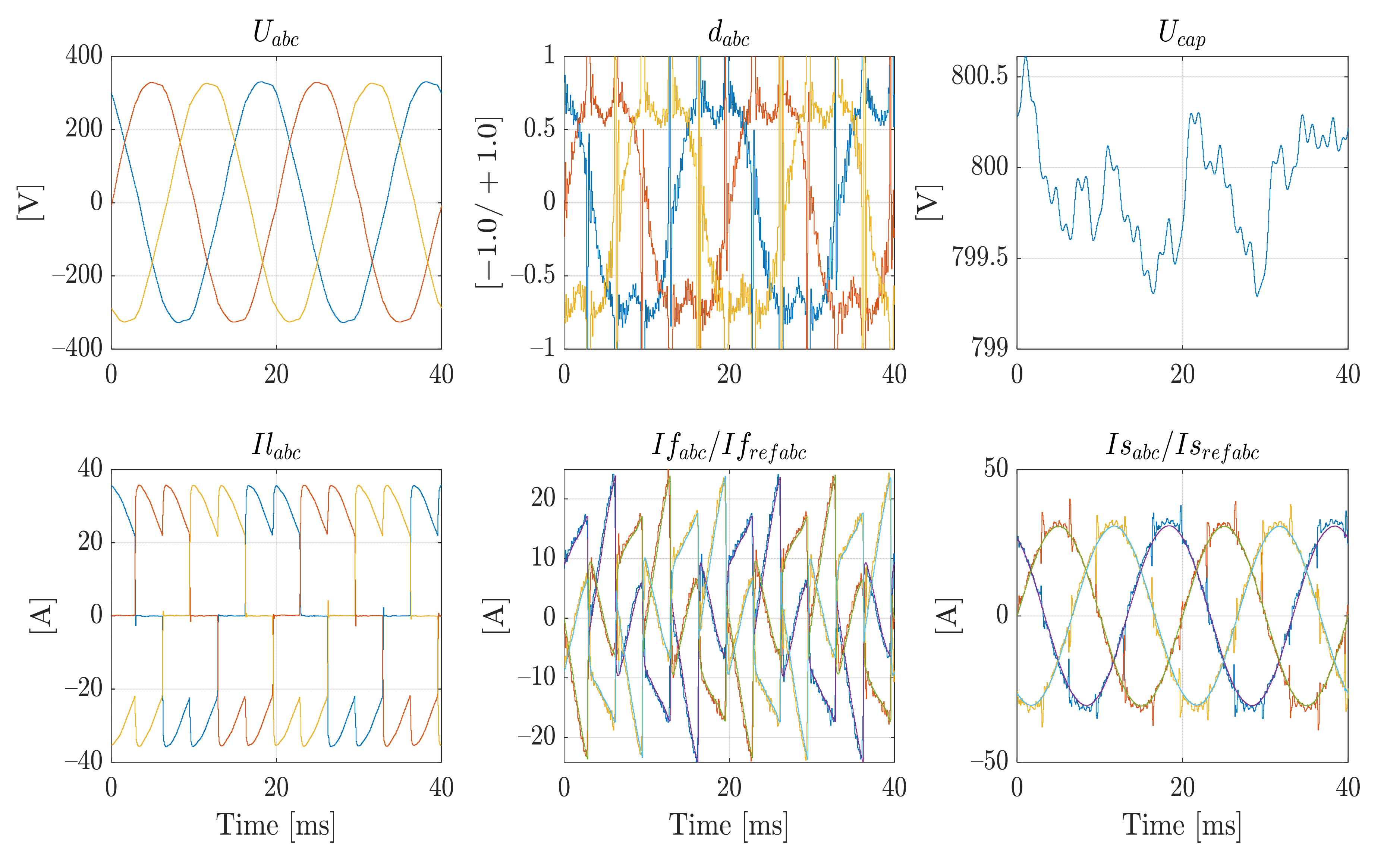
The results of the presented optimal controller are shown in Figure 11. It can be observed that there is a significant improvement in the shape of the grid current Is_abc in comparison to the PI controller. Of course, the optimal controller also sets the control at the limit levels, but these are the optimal values from the point of view of tracking the reference filter current. The control limit values correspond to the selection of controls located on the vertexes, edges, or planes of the control space defined by the constraints (6). The THD value of the grid currents is about 8.4%.

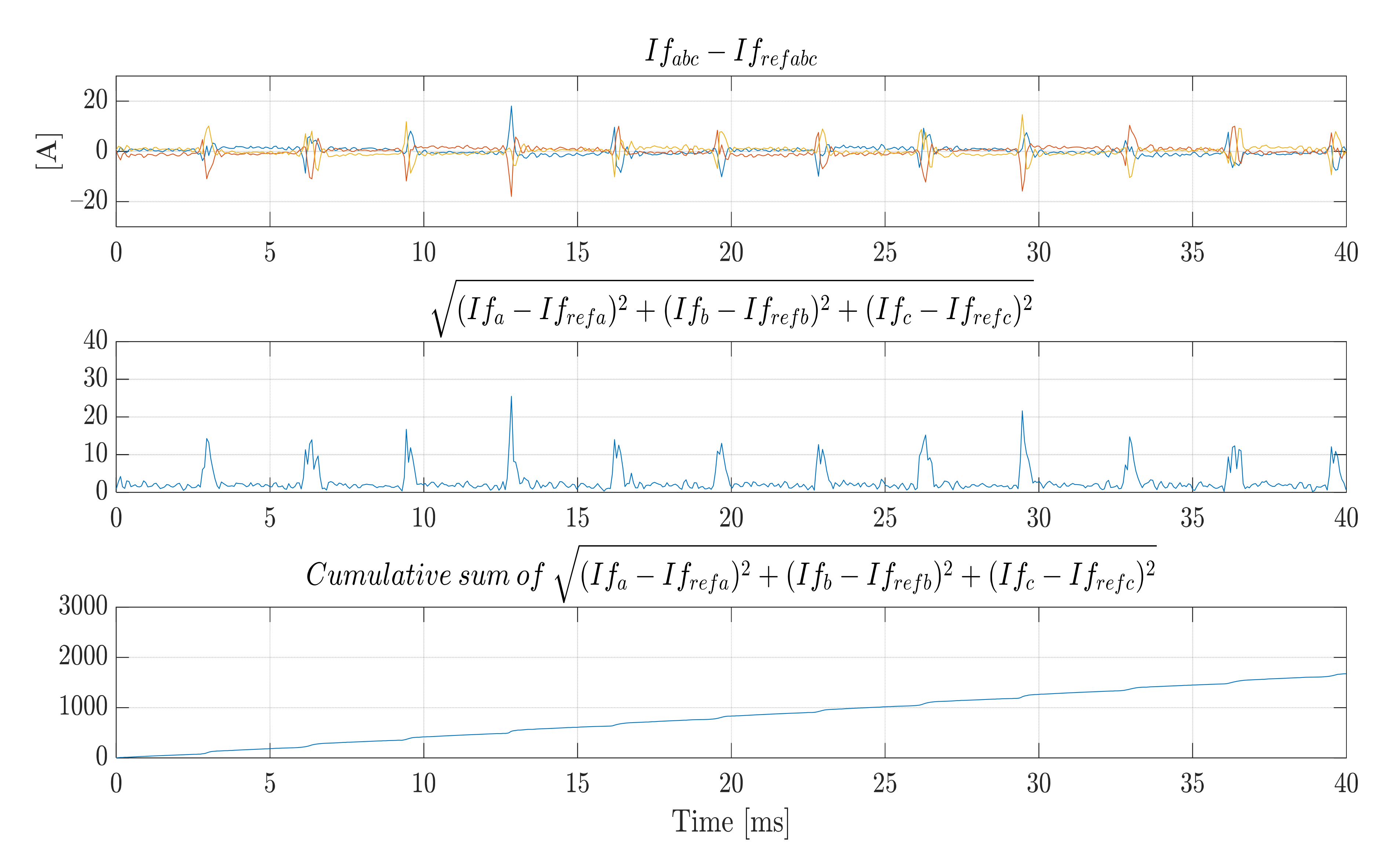
Figure 12 shows the control error. The cumulative control error (23) is equal to approximately 1680 in this case. The impact of the rapid commutation changes on the load currents is significantly lower than that presented in Figure 10.

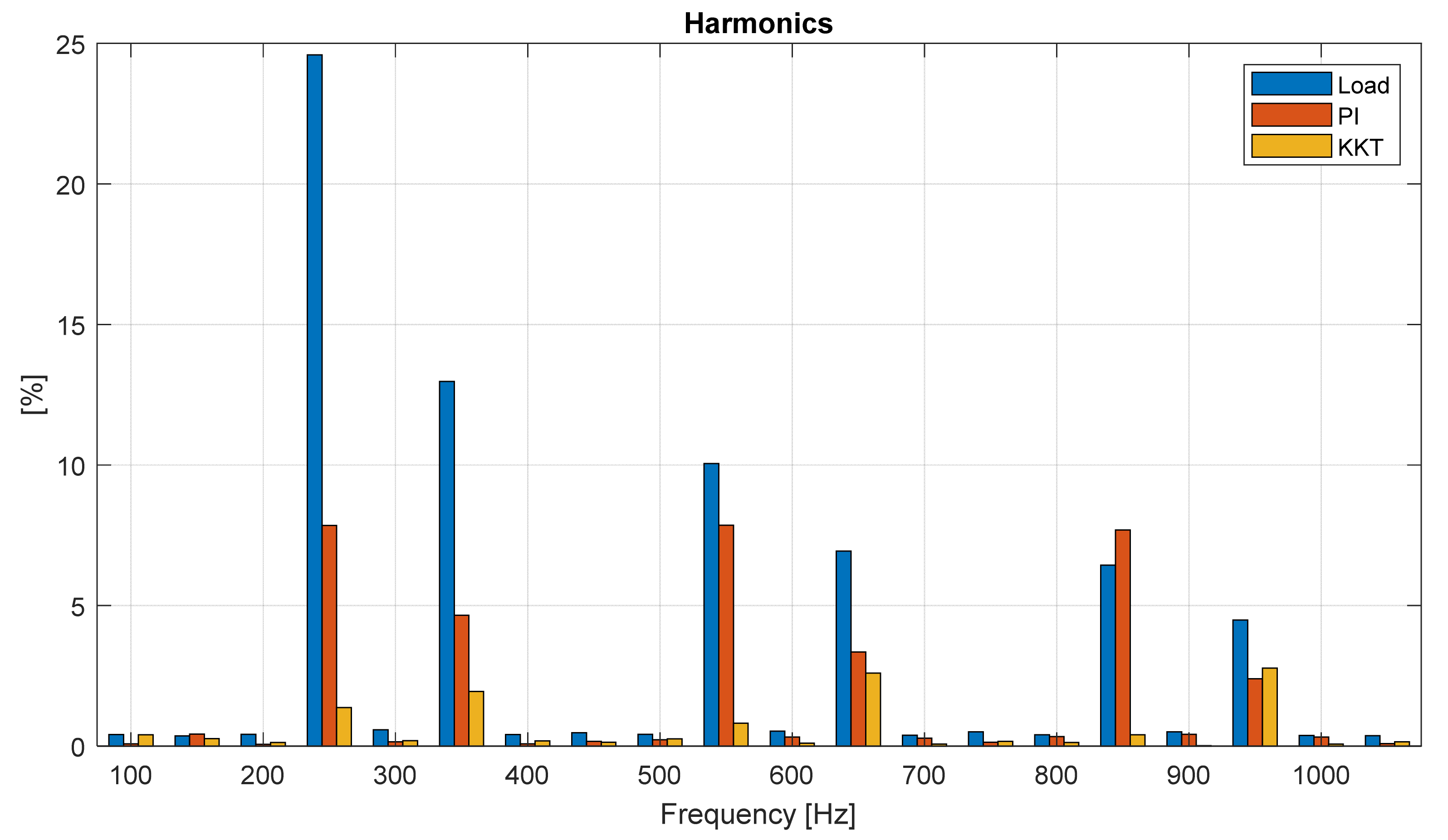
Figure 13 shows the percentage of harmonics in relation to the fundamental harmonic. One can notice a reduction in the level of harmonics; although, for the 17th harmonic (850 Hz), the optimal PI tracking controller increases the amplitude. There is also a more effective reduction in harmonics by the KKT controller, with the exclusion of the 19th harmonic where the PI controller is slightly more effective.

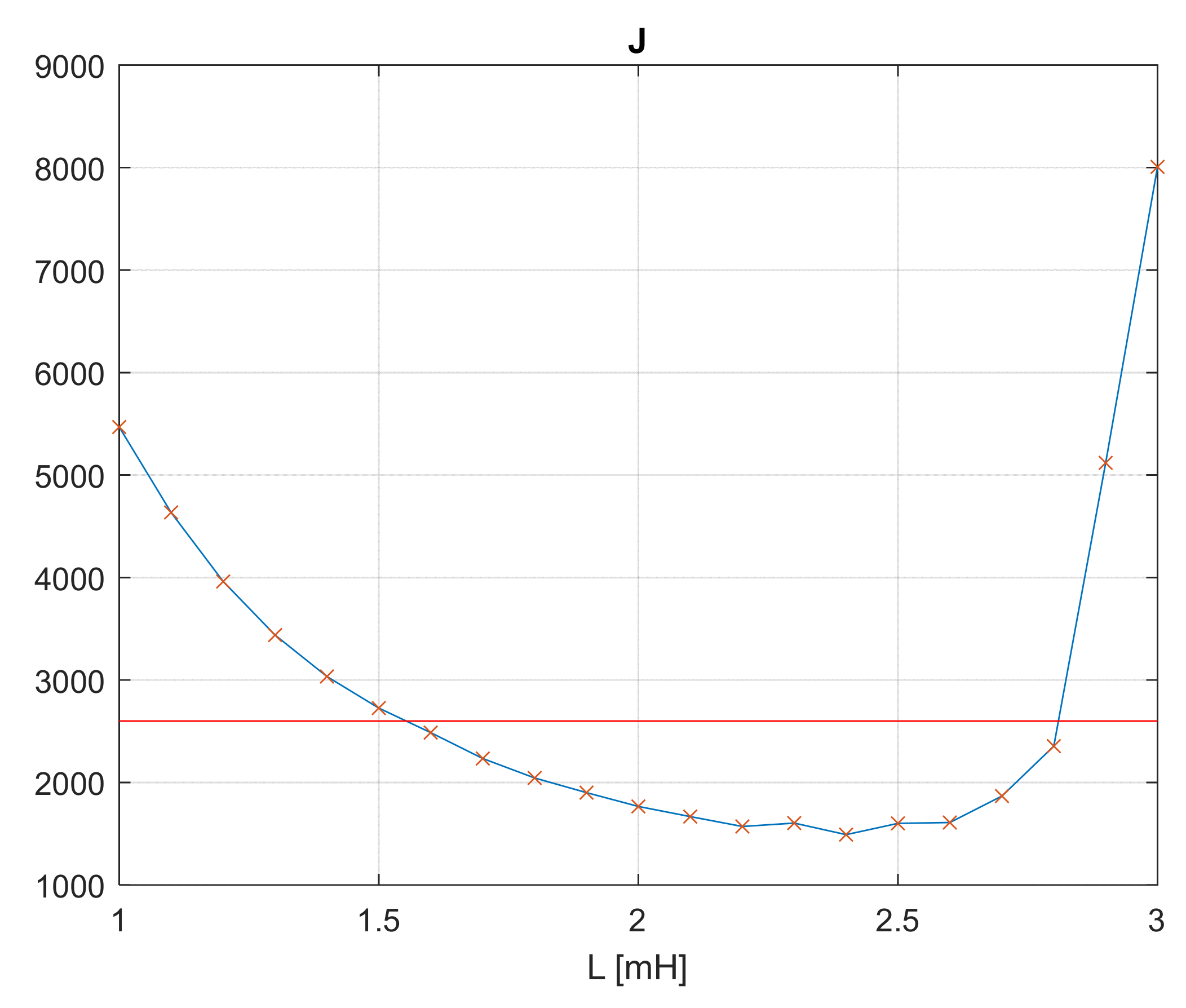
Inductance L is the only parameter of the proposed controller. However, filter inductance is not the only inductance that determines the rate of current change. Since the APF inductance value is small, the line inductance may influence the filter behavior. The grid impedance is much smaller than the L impedance of the APF in the vast majority of cases. Figure 14 shows the changes in the value of the quality factor (23) as a function of the L inductance of the controller given by formulas (20)–(22). As expected, a slight increase in the APF inductance improves the results. The most important feature of the proposed controller appears to be a flat criterion function around the optimal value of the L parameter, indicating a low sensitivity of the controller to the L parameter. If one takes the quality factor of the optimal PI controller equal to 2600 as a reference point, a change in the L parameter value in the range from 1.6 to 2.8 mH still provides a controller that is better than the PI controller.

5. Discussion and Conclusions

Most of control algorithms do not consider the effect of saturation on control signal. An example is PID controllers, during the analysis of which an unsaturated value of the controller output is assumed. In real situations, the controller always has a limited value of the output signal because of a limited power range that can be used to control the object. Tuning such controllers to obtain the optimal behavior in terms of a given quality criterion neglects the processes of entry and exit from the saturation state. Meanwhile, saturation is an important state because it allows an object to be controlled by the extreme power value; however, at the same time, it breaks the feedback loop because the output signal of the controller does not depend on the value of the input signals.

The control method that takes into account the saturation of the control values is Model Predictive Control (MPC). MPC algorithms calculate the optimal control in a given prediction horizon, taking into account the limits of control values and the limits of state variables. Convex state and input constraints and a convex objective function require a convex optimization numerical method to calculate the outputs of the MPC controller. The presented method behaves in the same way. Depending on the state of the S-APF, it is selected as the optimal control, including boundary controls. Optimal control minimizes the control error, resulting in the three currents approaching the setpoints. Contrary to MPC, the presented method does not solve the complex numerical optimization problem but uses the explicitly given formulas. Efficient quadratic programming algorithms that rapidly solve the MPC problem also exist. Unfortunately, the calculation time remains significantly longer than the 10–20 ms period, which a control system with a sampling period of 68 ms can spend on this calculation. The explicit control formulas given enable their use in real-time control with sampling frequencies of several dozen kilohertz. The presented comparison of the optimal PI and KKT algorithms proves a better operation of the KKT algorithm both in tracking reference currents and THD reduction in grid currents.

The formulas presented for calculating optimal control (20)–(22) are calculated on modern microprocessors within several dozens of microseconds. The experimental results presented in this paper used APF equipped with IGBT transistors. The control computation period and the control PWM signal period were equal to each other and equal to 68 ms. Modern power electronics systems use transistor bridges made of SiC and GaN technology, operating with switching frequencies of the order of megahertz. The conversion of the presented algorithm to a fixed-point form and its implementation in an FPGA fabric may be a challenging issue. Then, in the case of SiC and GaN bridges, it would be possible to calculate the optimal control with the switching frequency determined by the PWM control signal.

References

- Lumbreras, D.; Gálvez, E.; Collado, A.; Zaragoza, J. Trends in Power Quality, Harmonic Mitigation and Standards for Light and Heavy Industries: A Review. Energies 2020, 13, 5792. [Google Scholar] [CrossRef]
- Maciążek, M. Power theories applications to control active compensators. In Power Theories for Improved Power Quality; Benysek, G., Pasko, M., Eds.; Springer: London, UK, 2012; pp. 49–116. [Google Scholar]
- Putri, A.I.; Rizqiawan, A.; Rozzi, F.; Zakkia, N.; Haroen, Y.; Dahono, P.A. A hysteresis current controller for grid-connected inverter with reduced losses. In Proceedings of the 2016 2nd International Conference of Industrial, Mechanical, Electrical, and Chemical Engineering (ICIMECE), Yogyakarta, Indonesia, 6–7 October 2016; pp. 167–170. [Google Scholar]
- Panda, G.; Dash, S.K.; Sahoo, N.; Panda, G. Comparative performance analysis of Shunt Active power filter and Hybrid Active Power Filter using FPGA-based hysteresis current controller. In Proceedings of the 2012 IEEE 5th India International Conference on Power Electronics (IICPE), Delhi, India, 6–8 December 2012; pp. 1–6. [Google Scholar]
- Nguyen-Van, T.; Abe, R.; Tanaka, K. Digital Adaptive Hysteresis Current Control for Multi-Functional Inverters. Energies 2018, 11, 2422. [Google Scholar] [CrossRef] [Green Version]
- Jayasankar, V.N.; Vinatha, U. Backstepping Controller with Dual Self-Tuning Filter for Single-Phase Shunt Active Power Filters Under Distorted Grid Voltage Condition. IEEE Trans. Ind. Appl. 2020, 56, 7176–7184. [Google Scholar] [CrossRef]
- Singh, V.K.; Tripathi, R.N.; Hanamoto, T. HIL Co-Simulation of Finite Set-Model Predictive Control Using FPGA for a Three-Phase VSI System. Energies 2018, 11, 909. [Google Scholar] [CrossRef] [Green Version]
- Sun, X.; Tang, X. Current control of active power filters assisted by three-state hysteresis. In Proceedings of the 2015 5th International Conference on Electric Utility Deregulation and Restructuring and Power Technologies (DRPT), Changsha, China, 26–29 November 2015; pp. 2356–2359. [Google Scholar]
- Nachiappan, A.; Sundararajan, K.; Malarselvam, V. Current controlled voltage source inverter using Hysteresis controller and PI controller. In Proceedings of the 2012 International Conference on Power, Signals, Controls and Computation, Thrissur, India, 3–6 January 2012; pp. 1–6. [Google Scholar]
- Jena, S.; Babu, B.C.; Naik, A.K.; Mishra, G. Performance improvement of single-phase grid Connected PWM inverter using PI with hysteresis current controller. In Proceedings of the 2011 International Conference on Energy, Automation and Signal, Bhubaneswar, India, 28–30 December 2011; pp. 1–5. [Google Scholar]
- Deželak, K.; Bracinik, P.; Sredenšek, K.; Seme, S. Proportional-Integral Controllers Performance of a Grid-Connected Solar PV System with Particle Swarm Optimization and Ziegler–Nichols Tuning Method. Energies 2021, 14, 2516. [Google Scholar] [CrossRef]
- Danayiyen, Y.; Lee, K.; Choi, M.; Lee, Y.I. Model Predictive Control of Uninterruptible Power Supply with Robust Disturbance Observer. Energies 2019, 12, 2871. [Google Scholar] [CrossRef] [Green Version]
- Tarisciotti, L.; Formentini, A.; Gaeta, A.; Degano, M.; Zanchetta, P.; Rabbeni, R.; Pucci, M. Model Predictive Control for Shunt Active Filters WITH Fixed Switching Frequency. IEEE Trans. Ind. Appl. 2017, 53, 296–304. [Google Scholar] [CrossRef]
- Bosch, S.; Staiger, J.; Steinhart, H. Predictive Current Control for an Active Power Filter With LCL-Filter. IEEE Trans. Ind. Electron. 2018, 65, 4943–4952. [Google Scholar] [CrossRef]
- Krishna, R.; Kottayil, S.K.; Leijon, M. Predictive current controller for a grid connected three level inverter with reactive power control. In Proceedings of the 2010 IEEE 12th Workshop on Control and Modeling for Power Electronics (COMPEL), Boulder, CO, USA, 28–30 June 2010; pp. 1–6. [Google Scholar] [CrossRef]
- Bielecka, A.; Wojciechowski, D. Stability Analysis of Shunt Active Power Filter with Predictive Closed-Loop Control of Supply Current. Energies 2021, 14, 2208. [Google Scholar] [CrossRef]
- Jiang, W.; Ding, X.; Ni, Y.; Wang, J.; Wang, L.; Ma, W. An Improved Deadbeat Control for a Three-Phase Three-Line Active Power Filter With Current-Tracking Error Compensation. IEEE Trans. Power Electron. 2018, 33, 2061–2072. [Google Scholar] [CrossRef]
- Sou, W.-K.; Choi, W.-H.; Chao, C.-W.; Lam, C.-S.; Gong, C.; Wong, C.-K.; Wong, M.-C. A Deadbeat Current Controller of LC-Hybrid Active Power Filter for Power Quality Improvement. IEEE J. Emerg. Sel. Top. Power Electron. 2020, 8, 3891–3905. [Google Scholar] [CrossRef]
- Gong, C.; Sou, W.-K.; Lam, C.-S. Second-Order Sliding-Mode Current Controller for LC-Coupling Hybrid Active Power Filter. IEEE Trans. Ind. Electron. 2021, 68, 1883–1894. [Google Scholar] [CrossRef]
- Lopez-Caiza, D.; Flores-Bahamonde, F.; Kouro, S.; Santana, V.; Muller, N.; Chub, A. Sliding Mode Based Control of Dual Boost Inverter for Grid Connection. Energies 2019, 12, 4241. [Google Scholar] [CrossRef] [Green Version]
- Panigrahi, R.; Subudhi, B. Performance Enhancement of Shunt Active Power Filter Using a Kalman Filter-Based H∞ Control Strategy. IEEE Trans. Power Electron. 2016, 32, 2622–2630. [Google Scholar] [CrossRef]
- Suru, C.V.; Popescu, M.; Linca, M.; Stanculescu, A. Fuzzy Logic Controller Implementation for the Compensating Capacitor Voltage of an Indirect Current Controlled Active Filter. In Proceedings of the 2020 International Conference and Exposition on Electrical and Power Engineering (EPE), Iasi, Romania, 22–23 October 2020. [Google Scholar]
- Tan, K.-H.; Lin, F.-J.; Chen, J.-H. A Three-Phase Four-Leg Inverter-Based Active Power Filter for Unbalanced Current Compensation Using a Petri Probabilistic Fuzzy Neural Network. Energies 2017, 10, 2005. [Google Scholar] [CrossRef] [Green Version]
- Bouhouta, A.; Moulahoum, S.; Kabache, N.; Colak, I. Experimental Investigation of Fuzzy Logic Controller Based Indirect Current Control Algorithm for Shunt Active Power Filter. In Proceedings of the 2019 8th International Conference on Renewable Energy Research and Applications (ICRERA), Brasov, Romania, 3–6 November 2019. [Google Scholar]
- Dey, P.; Mekhilef, S. Current Controllers of Active Power Filter for Power Quality Improvement: A Technical Analysis. Automatika 2015, 56, 42–54. [Google Scholar] [CrossRef] [Green Version]
- Avnet: Quality Electronic Components & Services. Available online: https://www.avnet.com/wps/portal/us/products/avnet-boards (accessed on 15 July 2021).
- Kołek, K.; Piatek, K. Rapid algorithm prototyping and implementation for power quality measurement. EURASIP J. Adv. Signal Process. 2015, 2015, 968. [Google Scholar] [CrossRef] [Green Version]
- Kołek, K.; Piatek, K.; Firlit, A. Rapid controller development for a dynamic voltage restorer. In Proceedings of the 2017 International Symposium ELMAR, Zadar, Croatia, 18–20 September 2017; pp. 237–240. [Google Scholar] [CrossRef]
- Firlit, A.; Kołek, K.; Piatek, K. Heterogeneous active power filter controller. In Proceedings of the 2017 International Symposium ELMAR, Zadar, Croatia, 18–20 September 2017; pp. 241–244. [Google Scholar] [CrossRef]
Figure 1.
Functional diagram of the S-APF.
Figure 2.
PWM generation from the control signals.
Figure 3.
Equivalent configurations for the first phase.
Figure 4.
APF controller.
Figure 5.
Architecture of the S-APF controller.
Figure 6.
Automatic generation of real-time application.
Figure 7.
The S-APF that was used for testing (APF-100/xxx/3W—courtesy of ELSTA Elektronika, Wieliczka, Poland).
Figure 8.
Cost function vs. parameters of the PI controller.
Figure 9.
Results of the PI controller.
Figure 10.
Error and quality factor of the PI controller.
Figure 11.
Results of the optimal controller.
Figure 12.
Error and quality factor of the optimal controller.
Figure 13.
The currents spectra of the selected phase (up to 1 kHz): blue—the load current; red—the grid current for the PI optimal controller; yellow—the grid current for the KKT controller.
Figure 14.
Penalty function vs. parameter L of the KKT controller.
Publisher’s Note: MDPI stays neutral with regard to jurisdictional claims in published maps and institutional affiliations. |
© 2021 by the authors. Licensee MDPI, Basel, Switzerland. This article is an open access article distributed under the terms and conditions of the Creative Commons Attribution (CC BY) license (https://creativecommons.org/licenses/by/4.0/).
Share and Cite
MDPI and ACS Style
Kołek, K.; Firlit, A. A New Optimal Current Controller for a Three-Phase Shunt Active Power Filter Based on Karush–Kuhn–Tucker Conditions. Energies 2021, 14, 6381. https://doi.org/10.3390/en14196381
AMA Style
Kołek K, Firlit A. A New Optimal Current Controller for a Three-Phase Shunt Active Power Filter Based on Karush–Kuhn–Tucker Conditions. Energies. 2021; 14(19):6381. https://doi.org/10.3390/en14196381
Chicago/Turabian StyleKołek, Krzysztof, and Andrzej Firlit. 2021. "A New Optimal Current Controller for a Three-Phase Shunt Active Power Filter Based on Karush–Kuhn–Tucker Conditions" Energies 14, no. 19: 6381. https://doi.org/10.3390/en14196381
Note that from the first issue of 2016, this journal uses article numbers instead of page numbers. See further details here.