Abstract
Wind power penetration has increased rapidly in recent years. In winter, the wind turbine blade imbalance fault caused by ice accretion increase the maintenance costs of wind farms. It is necessary to detect the fault before blade breakage occurs. Preliminary analysis of time series simulation data shows that it is difficult to detect the imbalance faults by traditional mathematical methods, as there is little difference between normal and fault conditions. A deep learning method for wind turbine blade imbalance fault detection and classification is proposed in this paper. A long short-term memory (LSTM) neural network model is built to extract the characteristics of the fault signal. The attention mechanism is built into the LSTM to increase its performance. The simulation results show that the proposed approach can detect the imbalance fault with an accuracy of over 98%, which proves the effectiveness of the proposed approach on wind turbine blade imbalance fault detection.
1. Introduction
As a clean and renewable energy, wind power has developed rapidly in recent years [1]. With the increasing penetration of wind power, the problems of high maintenance costs of wind turbines and high failure rate have been highlighted [2,3]. Forty percent of the maintenance cost of a wind farm is related to wind turbine component failure [4,5]. Wind turbines are generally installed on the mountain or along the coastline, thus it is difficult to obtain the daily operating state of wind turbines. Wind turbine failure mainly includes the mechanical failure of the gearbox, various bearing and rotor [6], breakage of blades [7], an abnormal working state of generator and power electronics [8], etc. When the wind turbines fail, the fault of which will arise power oscillation in the power system. These problems lead to high maintenance costs and damage to the power grid. Therefore, it is necessary to diagnose the potential danger of wind turbines to avoid more serious accidents before the wind turbine has a devastating failure [9,10].
Traditional fault diagnosis methods are sensor-based monitoring. Installing a large number of sensors in different parts of the wind turbine increases the investment cost. Therefore, it is necessary to apply a more effective data-driven method in fault diagnosis to reduce the investment costs [11]. Various methods have been proposed in literature to solve this problem: Fault detection based on the improved temporal constraint network method [12], the history-driven differential evolution approach [13], cointegration residuals analysis [14], generator current signals [15], and machine learning method [16], etc. The machine learning-based approach has especially been applied in many fields in recent years. Deep learning (DL) is one of the most important parts of this hot topic. Google’s AlphaGo [17] and AlphaGo Zero [18] use the deep neural network to train themselves, and have had great breakthroughs in recent years. Because of the great learning ability of DL, it can also be applied in a power system.
Since 2006, DL has appeared as a new research field in machine learning research field [19]. DL can be used to extract the features of a large number of data [20,21,22]. Due to the high calculation costs and the features being difficult to be extracted, it is not applicable to obtain the features by using traditional mathematical methods [21]. Various DL-based approaches have been proposed in literature for wind turbine fault detection due to the strong feature extraction ability of DL [23]. In general, the fault detection of the DL-based approach consists of two steps: First, one extracts the fault features by neural network, and second, one realizes the classification based on the extracted features [24]. Reference [25] applied the sparse auto-encoder in fault detection of the wind power system transmission line, which realized the wind farm transmission line faults identification, with an accuracy of 99%. A neural network-based approach for gearbox bearings fault detection was proposed in [26]. Study [27] successfully applied an auto-encoder-based method in wind turbine gearbox fault diagnosis. Convolutional neural network is used in fault detection of the wind turbine gearbox [28]. A deep auto-encoder-based method for wind turbine blade breakage diagnose is proposed in study [29], and the accuracies of the detection results reach 100%. All these prove that the application of DL in a power system is feasible. The imbalance fault caused by icing on wind turbine blades is difficult to detect. It is necessary to find a feasible method to detect the fault.
This paper proposes a new method for the wind turbine blade fault detection by combining long short-term memory (LSTM) with the attention mechanism. The contributions of this paper are as follows:
- (1)
- This paper proposes a data-driven method to solve the imbalance fault detection of wind turbine blades which considers the imbalance faults caused by the ice accretion.
- (2)
- A novel method based on LSTM and attention mechanism is proposed to solve the problem of wind turbine blade imbalance fault diagnosis, and it overcomes the problem that traditional methods have in extracting fault features.
The rest of this paper is structured as follows. Section 2 presents the working condition and the imbalance fault of wind turbine. The deep learning framework and the fault diagnosis method are shown in Section 3. Section 4 presents the case study of this research. Finally, the conclusion and summary of this paper is shown in Section 5.
2. Wind Turbines Imbalance Fault
The imbalance fault of wind turbine blades accounts for the majority of the wind turbine failures [4]. Under ideal conditions, the quality of the three wind turbine blades is equal. However, the mass of the wind turbine blades is imbalanced in real-world scenarios due to various factors. For example:
- (a)
- Due to the technical problems in the production process, there are some mass errors among the blades.
- (b)
- Wind turbines are usually installed at heights of tens or even hundreds of meters and the locations are usually at the peaks of mountains or offshore. Wind turbine blades will be corroded by exposure to harsh environments for a long time, which causes the imbalance of wind turbine blades.
- (c)
- In addition, in dusty or extreme cold weather conditions, wind turbine blades will be covered with dust or ice. When the dust or ice accumulates to a certain level, the imbalance fault of wind turbines will occur.
This paper assumes that the imbalance faults of a wind turbine are caused by the wind turbine blades, which are covered with ice. Wind turbines operate at variable wind speed conditions and the wind speed curve is shown in the following Figure 1.
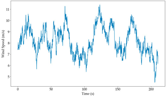
Figure 1.
The variable wind speed of test data.
In this research, in order to obtain the data of the wind turbine under different conditions, a 2MW wind turbine with a doubly fed induction generator (DFIG) was built by G. H. Bladed simulation software to verify the proposed method [30,31]. Figure 1 shows that the wind turbines were operating under the variable wind speed which ranges from 4 to 11 m/s. Under this condition, the output power curves of the wind turbine in normal state and fault state are shown in Figure 2.
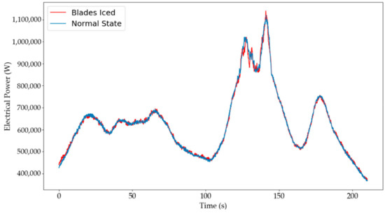
Figure 2.
The output power curves of the wind turbine: Blue line represents the output electrical power of normal state under the variable wind speed. Red line presents the output electrical power of blade in iced fault state under the variable wind speed.
It shows that the trends of the two curves are almost the same and it is difficult for traditional fault analysis methods to distinguish the difference between normal state and iced state. Compared with the traditional mathematical methods, this study adopts a neural network, which has proved to be effective in extracting features and detecting the imbalance faults of wind turbine. At the same time, the method of neural network could also reduce the calculation costs.
3. Deep Learning Framework and Training Process
A DL framework is shown in this section. Traditional DL mainly includes the following basic network frameworks: fully connected neural network (FNN), convolutional neural network (CNN) and recurrent neural network (RNN) [20]. RNN has advantages in processing time series data, LSTM is an improved version of RNN and is good at extracting long-term dependency features. LSTM is used to extract features in the proposed approach of this paper. Compared with ordinary neural networks, LSTM network can solve the vanishing gradient problem [32]. In addition, LSTM is outstanding in feature extraction from temporal dependencies data [33]. When processing the time series data, LSTM has high efficiency in the field of machine learning [34,35]. But with the length of data increasing, LSTM has difficulty in feature extracting [33]. In order to enhance the learning ability of LSTM, this study adds the attention mechanism after LSTM. The attention mechanism helps LSTM learn the temporal dependencies data [36].
The DL framework proposed in this paper contains two parts: LSTM and attention mechanism. The details are described in the following subsections respectively.
3.1. Recurrent Neural Network (RNN)
RNN is a neural network with a special structure. Compared with FNN and CNN, RNN can be regarded as a network with memory. It stores the features of the previous moment which is used as the next moment’s input. Thus RNN can better obtain the characteristics of time series data than CNN and FNN.
A simple RNN include 3 layers: Input layer, hidden layer and output layer. The standard RNN structure is shown in Figure 3:
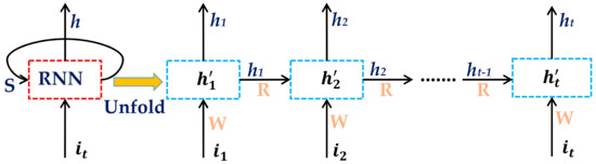
Figure 3.
A simple unfold recurrent neural network (RNN) structure.
Where represents the input vector at the t-th moment. In hidden layers, every cell A has an activation function. At each time step of the model, the RNN cell outputs an eigenvalue, which will be sent to the next cell. The specific function of RNN is shown in Equations (1) and (2):
where represents the hidden state of the neural network at time t; and represent the weight matrices and the bias vector, respectively. is the output of the t-th RNN cell and is the activation function. Because of this structure, RNN has memory function that can memorize the features of the time series data.
The learning ability of RNN decreases with the increase of dimension and amount of data, however, LSTM can solve this disadvantage of RNN.
3.2. The Overall Framework
In Section 2, preliminary analysis shows that the features of the fault data are not obvious enough. In order to detect the fault effectively, the combination of LSTM and attention mechanism to realize wind turbines imbalance fault detection and classification is a feasible option.
In order to make the neural network more sensitive to the wind turbine imbalance faults, this paper also considers other parameters of wind turbines, not including power and current, which are shown in Equation (3), where is the hub wind speed magnitude, ω is the rotor speed, is the electrical power, is the turbine current and is the generator torque. The , , , and are all column vectors. In order to obtain the torque information during wind turbine blade rotation and better reflect the operation characteristics of the wind turbine, the sampling time interval of wind turbine data in this research is 0.08 s.
The overall structure of the imbalance fault detection is shown in Figure 4. It shows that the attention mechanism is added after the output of LSTM cells, and the softmax function completes the fault detection.
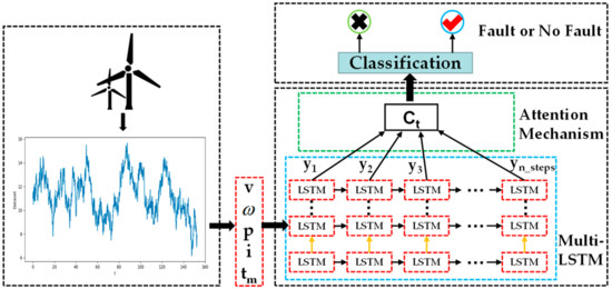
Figure 4.
The overall structure of the imbalance fault detection.
3.2.1. LSTM
Since standard RNN just thinks about neighboring states, if the state is too far from the current RNN, the data may be forgotten which could lead the neural network loss learning ability. However, the LSTM doesn’t have that problem. Compared with RNN, LSTM has added three special gates in its cell, the forget gate, input gate and output gate. The inner structure of LSTM is shown in Figure 5. The most important part to the LSTM network is the cell state [37]. The LSTM can control the three gates to decide whether the outside data should be written in the cell or not.
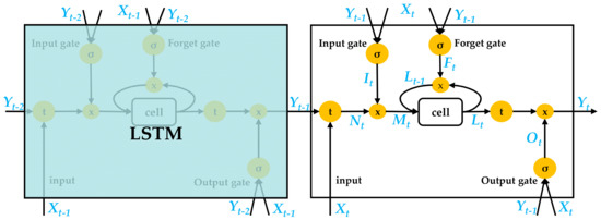
Figure 5.
The inner structure of long short-term memory (LSTM), where a circle with a σ represents an activation function and a circle with a x represents multiply function. , , are the output information of input, forget and output gates; and these three control value are all connected with the input and the output of the previous moment .
The functions of these three gates are shown in Equations (4)–(6), respectively,
where the activation function σ is sigmoid function, and , , , , and are the weight of each gate respectively, the shapes of which are all matrices, and , , are the biases vector of these three gates. The input data is show as Equation (7),
where is the activation function, tanh, and are the weight matrices, and is the input biases vector. After obtaining the three gates state and the input information, the intermediate variable can be described as below:
where denotes matrix multiplication. The state value of input gate, , is range from 0 to 1, it determines proportionately how much input to pass to the next step. Therefore, the LSTM cell information and the output state can be formulated as Equations (9) and (10). Like , the state value of forget gate and output gate, and , both range from 0 to 1.
After getting the output information of the LSTM, they all will be sent into the attention mechanism for further processing. Attention mechanism multiplies different time series data by a weight coefficient then obtains the final dynamic characteristics.
In this research, the updating of training parameters is based on gradient descent method and the specific algorithms are shown as below:
where and represent the new weights , , , or , , , after updating of the neural network. Similarly, represents the new bias of the network. , and are the weights and bias of the previous training. is the learning rate of the neural network and is the loss function value. In this research, the loss function of the model is sparse softmax cross entropy with logits [38]. This loss function is a combination of softmax and cross entropy functions. Comparing with softmax cross entropy with logits and cross entropy, the calculation speed of the selected function is faster.
3.2.2. Attention Mechanism
When dealing with long input sequence, only the output of the LSTM neural network, , is used as the information representation of the entire input sequence, that means all information of the input sequence is compressed into a fixed length vector. As the length of the input sequence continues to increase, the ability of the overall model to process information will be limited and weakened. In order to solve this problem, this research has introduced the attention mechanism in the decoding phase. Attention mechanism can be considered as a simple three-layer neural network, which includes input layer, hidden layer and output layer. The input in this paper is the last layer’s output of a multi-layer LSTM, which is a vector and the length of this vector is equal to the time steps of LSTM.
Attention mechanism has great advantages on time series learning, and the core goal of attention mechanism is turning the fixed output into a dynamic context vector . Its characteristic equation can be broken down into the following three steps:
- The first step is calculating the parameter at i-th time, , which is described as Equation (14):where is a model which scores how well the input of i-th moment and the output of t-th moment match, , , . are the pending training parameters, and tanh is the activation function.
- The second step is normalizing the data obtained at step one, then getting the weight score of each state, which is shown as Equation (15),where is a weight coefficient, which is the normalized probability distribution of at each time step based on Equation (14).
- Obtaining the dynamic characteristics vector by multiplying the output of LSTM by the probability, which is shown in Equation (16),
After getting the dynamic context vector , the process of decoding is almost the same as the traditional sequence classification based on LSTM.
3.3. The Training Process
The training process of the algorithm is shown as in Table 1. All parameters have been described in the previous subsection.

Table 1.
The training process of the algorithm of the neural network.
More details regarding the working principle of the proposed method can be described as follows: Firstly, the raw data of wind turbine under normal and imbalance fault operation state are generated by simulation software. The shape of raw data is a two dimensional matrix: , which has been described in Equation (3). But the shape of input data of LSTM must be a three-dimensional array, so that the first task of the model need to do is reshape the raw data into a three dimensional array of shape [batch size, time step, n-inputs], where batch size and time step are the training parameters of the neural network and can be adjusted, and n-inputs represents the number of different kinds of wind turbine operation data, which in this paper is five. After the raw data has been reshaped, one then mixes fault data with normal data as the dataset of the model. The dataset will be randomly divided into a training set and testing set. Finally, after learning the features of these dataset, the model can classify the fault signals and normal signals by sparse softmax cross entropy with logits function.
4. Case Study
This paper uses the G. H. Bladed software to simulate the wind power generator with different kinds of imbalance fault, then collects the main information by this software to do the following data processing. This study randomly chooses the 80% of each dataset as a training set, and the remaining 20% of the dataset is divided into 10% for the validation set and 10% for the testing set.
Hardware environment and software platform: The training of network is completed on a PC with Intel(R) Core i9-7900X @ 3.30GHz CPU, 64G DDR4 RAM and Nvidia GeForce RTX 2080 Ti (11GB VRAM). And the software platforms are WINDOWS-10 (Professional) operating system and Pycharm 3.6 (64 bit). This paper uses the GPU version of TensorFlow to build the LSTM neural network and accelerate the hardware.
Data pre-processing: Firstly, add different labels to the different imbalance faults data obtained from G. H. Bladed. Then divide the data into appropriate time-step length as a batch.
4.1. Experimental Results
Figure 6 shows that the imbalance fault occurs at the 10,000th sampling points and disappears at the 20,000th points. Figure 7 shows that when the imbalanced fault is detected, the model gives a pulse signal with a value of 1. When the fault disappears, the value of the pulse drops to 0. Because of signal transmission and data calculation, there will be a short time (1.8 s) delay which is shown in Figure 7.
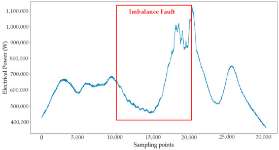
Figure 6.
Imbalance fault occurs from the 10,000th to 20,000th sampling points.
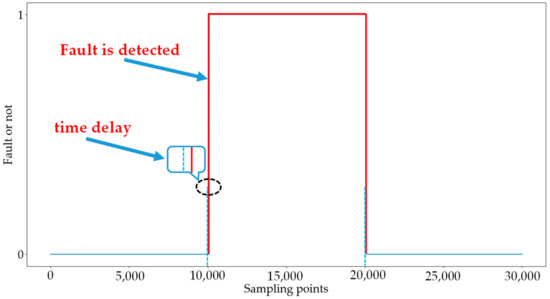
Figure 7.
The fault is detected by the proposed model.
In order to prove the feasibility of the proposed method, this paper provides the detection results under different imbalanced fault conditions. The number of iced wind turbine blades ranges from one to three and the mass of ice is also variable. The detection results of network under one wind turbine blade iced condition are shown in Figure 8, and the parameter of imbalance fault is obtained every 200 iterations. The fault detection accuracy of the neural network is more than 99%. The result shows that the proposed DL-based approach is effective in detecting the wind turbine fault.
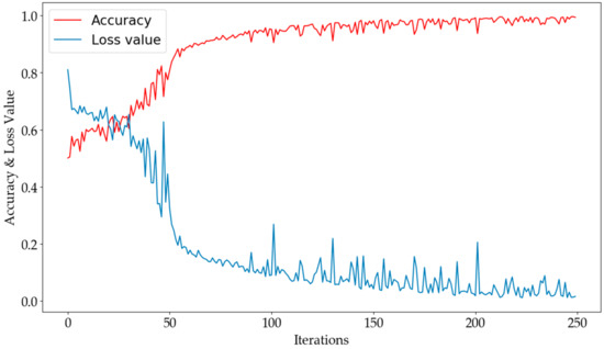
Figure 8.
The accuracy and loss value of the neural network.
The accuracies of a neural network with 256 attention size and the accuracy of LSTM without attention mechanism are shown in Figure 9. It can be observed that LSTM combined with attention mechanism can increase the convergence rate. In the early stages, the accuracy of the neural network with attention mechanism hardly changes but the accuracy of the network without attention mechanism slowly rises. As the attention mechanism can hold more features of the time series data, when the network finds the best gradient descent direction, the accuracy of the neural network with attention mechanism rises rapidly. Finally, the accuracy of the network model with attention mechanism is higher than the LSTM without attention mechanism. It proves that the performance of the neural network can be improved by adding attention mechanism.
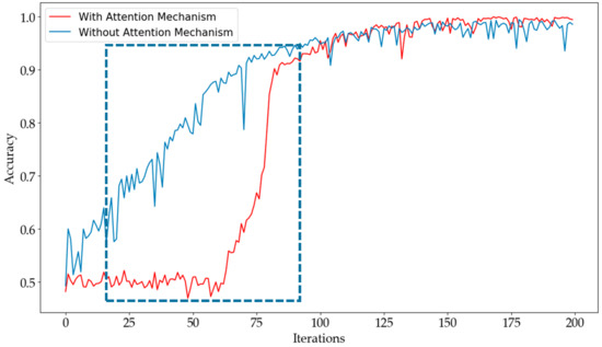
Figure 9.
The accuracy curves: The red curve is the accuracy of model with 256 attention size, and the blue curve is the accuracy of LSTM without attention mechanism.
The accuracies of neural network with different attention size are listed in Table 2. With the increase in attention size, the accuracies of neural network increase. The results in this research show that the best attention size of LSTM combines with attention mechanism is 256, the accuracy of which reaches 99.8%.
Table 2.
The accuracies of models with different attention size.
The accuracies of the neural network with different time-step are shown in Figure 10. It can be observed that in the early stage of the learning process, the accuracy of model with one time-step rises rapidly; but in the end, the accuracy of model with only one time-step is much lower than others with a larger time-step. The reason for this phenomenon is that the datasets are temporal dependencies and only one time-step leads the neural networks can’t obtain the temporal correlation characteristics commendably.
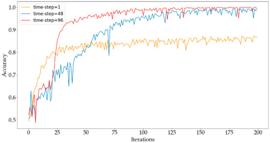
Figure 10.
The accuracies of neural network with different time-step under two blades with ice accretion condition.
The accuracies of models with different time-step length are listed in Table 3. With the increase of time-step, the accuracy of network also increases.
Table 3.
The accuracies of models with different time-step.
The accuracies of models with different batch size are listed in Table 4. It shows that the highest accuracy of neural networks with batch size of 48 is not more than 88%. Because the batch size of the dataset will determine the direction of gradient descent, a too small batch of dataset will make the direction of gradient descent uncertain, which decreases the learning ability of the neural network. When the batch size of the model increases, the accuracy improves significantly.
Table 4.
The accuracies of models with different batch size.
It can be observed from Table 3 and Table 4 that time-step and batch-size are important parameters for neural network: When their values are too large, the memory is heavily occupied and the training time of neural networks increase significantly. The best time-step and batch size of the model in this paper are 96 and 4096 respectively.
When the mass of ice accretion of the wind turbine blades increases, the features of imbalance fault of wind turbine blades are becoming more and more obvious. Compared with 15 kg, the accuracy curves of model with 15 kg and 30 kg ice accretion of each blade are shown in Figure 11. It shows that the accuracy of 30 kg ice accretion of each blades reaches 100%.
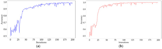
Figure 11.
The accuracies of models under different mass of ice accretion condition: (a) 15 kg ice on each blade, (b) 30 kg ice on each blade.
4.2. Methods Comparison
In order to prove the validity of the method proposed in this paper, this simulation compares the proposed method with standard RNN network. Take the icing on the surface of two blades of a wind turbine as an example, the results of a standard RNN compared with the LSTM with attention mechanism (LSTMAM) are shown in Figure 12.
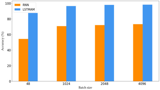
Figure 12.
The accuracies of recurrent neural network (RNN) and LSTM with attention mechanism (LSTMAM) with different Batch size.
It is obvious that in Figure 12, no matter how the batch size increases, the accuracies of RNN are no more than 74%; but the lowest accuracy of the proposed method is 87.5%. This paper also compares the proposed method with other methods, such as support vector machines (SVM) and Gaussian processes classification (GPC). Take the icing on the surface of two blades of a wind turbine as an example, the results are shown in Table 5. It shows that the accuracies of SVM and GPC are much lower than LSTMAM. Because traditional SVM and GPC are applicable to a small-scale dataset, but when the dimension and complexity of data increase, it is difficult to classify the faults by these methods. The results show that the proposed method outperforms various benchmark methods.
Table 5.
The accuracies of different methods.
A high sampling frequency is required in this research. When the imbalance fault occurs, the variation will occur on the low speed shaft torque and the rotating frequency of shaft is called 1 P [39]. Meanwhile, there is the fluctuation on aerodynamic torque on hub and effect on rotor speed caused by tower shadow. The spectra of the shaft torque or the output electric power of wind turbine with three blades will have fluctuation at 3 P frequency, which is three times the shaft rotating frequency. It is necessary to judge the frequency of 1 P and 3 P to detect whether the wind turbine has imbalance fault. The rotor speed of the wind turbine shown in this research is from 9 to 18 r/min, which corresponds to the 1 P and 3 P oscillation frequency from 0.15 to 0.3 and 0.45 to 0.9 Hz respectively. And the sampling frequency in this research is 12.5 Hz. According to Nyquist Sampling Theory [40], if the sampling frequency is too low, it is difficult to observe 1 P and 3 P frequency, which leads to inaccurate or the inability to detect the fault by the proposed method.
The noise of raw data can influence the learning of neural networks, which makes the model misjudge the signal. There are some artificial intelligence methods which can deal with the noise problem and with relatively mature technology, such as the auto-encoder [41], variational auto-encoder, stacked denoising auto-encoder [42], etc. These methods can effectively improve the robustness of the model to the noise.
5. Conclusions
This paper proposes an DL-based method which combines LSTM and an attention mechanism for wind turbine imbalance fault detection and classification. Compared with the standard LSTM, combining the LSTM and an attention mechanism can improve the learning ability and the convergence rate. This paper not only analyzes the voltage and current signals, but also considers other factors, such as wind speed and the torque of the hub in the dataset. Furthermore, compared with standard RNN, SVM and Gaussian Processes classification methods, the proposed method has a better performance in imbalance fault detection. The simulation results show that the proposed method is feasible in wind turbine blade imbalance detection and the highest accuracy of the proposed method is 100%.
Author Contributions
Conceptualization, W.H., D.C., J.C. and Q.H.; Methodology, W.H., D.C. and J.C.; Software, D.C. and J.C.; Validation, D.C. and J.C.; Formal Analysis, W.H., D.C., J.C. and B.Z.; Investigation, D.C. and J.C.; Data Curation, W.H and J.C.; Writing-Original Draft Preparation, D.C. and J.C.; Writing-Review & Editing, W.H., F.B., B.Z. and D.C.; Visualization, D.C. and J.C.; Supervision, W.H., Z.C. and F.B.
Funding
This research was funded by the National Natural Science Foundation of China, grant number 51707029.
Acknowledgments
The authors gratefully acknowledge the National Natural Science Foundation of China and appreciate the insightful comments and suggestions from the reviewers and the editor.
Conflicts of Interest
The authors declare no conflict of interest.
References
- Salvador, S.; Costoya, X.; Sanz-Larruga, F.; Gimeno, L. Development of Offshore Wind Power: Contrasting Optimal Wind Sites with Legal Restrictions in Galicia, Spain. Energies 2018, 11, 731. [Google Scholar] [CrossRef]
- Zhao, M.; Jiang, D.; Li, S. Research on fault mechanism of icing of wind turbine blades. In Proceedings of the 2nd World Non-Grid-Connected Wind Power and Energy Conference, Nanjing, China, 11–12 September 2009. [Google Scholar]
- Wang, N.; Li, J.; Hu, W.; Zhang, B.; Huang, Q.; Chen, Z. Optimal reactive power dispatch of a full-scale converter based wind farm considering loss minimization. Renew. Energy 2019, 139, 292–301. [Google Scholar] [CrossRef]
- Entezami, M.; Hillmansen, S.; Weston, P.; Papaelias, M.P. Fault detection and diagnosis within a wind turbine mechanical braking system using condition monitoring. Renew. Energy 2012, 47, 175–182. [Google Scholar] [CrossRef]
- Li, J.; Wang, N.; Zhou, D.; Hu, W.; Huang, Q.; Chen, Z.; Blaabjerg, F. Optimal Reactive Power Dispatch of Permanent Magnet Synchronous Generator-Based Wind Farm Considering Levelised Production Cost Minimisation. Renew. Energy 2019, 145, 1–12. [Google Scholar] [CrossRef]
- Tabatabaeipour, S.M.; Odgaard, P.F.; Bak, T.; Stoustrup, J. Fault Detection of Wind Turbines with Uncertain Parameters: A Set-Membership Approach. Energies 2012, 11, 2424–2448. [Google Scholar] [CrossRef]
- Hur, S.; Recalde-Camacho, L.; Leithead, W.E. Detection and compensation of anomalous conditions in a wind turbine. Energy 2017, 124, 74–86. [Google Scholar] [CrossRef]
- Yang, W.; Liu, C.; Jiang, D. An unsupervised spatiotemporal graphical modeling approach for wind turbine condition monitoring. Renew. Energy 2018, 127, 230–241. [Google Scholar] [CrossRef]
- Hameed, Z.; Hong, Y.S.; Cho, Y.M.; Ahn, S.H.; Song, C.K. Condition monitoring and fault detection of wind turbines and related algorithms: A review. Renew. Sustain. Energy Rev. 2009, 13, 1–39. [Google Scholar] [CrossRef]
- Ozgener, O.; Ozgener, L. Exergy and reliability analysis of wind turbine systems: A case study. Renew. Sustain. Energy Rev. 2007, 11, 1811–1826. [Google Scholar] [CrossRef]
- Deng, F.; Chen, Z.; Khan, M.R.; Zhu, R. Fault Detection and Localization Method for Modular Multilevel Converters. IEEE Trans. Power Electron. 2015, 30, 2721–2732. [Google Scholar] [CrossRef]
- Cui, Y.; Shi, J.; Wang, Z. Power System Fault Reasoning and Diagnosis Based on the Improved Temporal Constraint Network. IEEE Trans. Power Deliv. 2016, 31, 946–954. [Google Scholar] [CrossRef]
- Zhao, J.; Xu, Y.; Luo, F.; Dong, Z.Y.; Peng, Y. Power system fault diagnosis based on history driven differential evolution and stochastic time domain simulation. Inf. Sci. 2014, 275, 13–29. [Google Scholar] [CrossRef]
- Dao, P.B.; Staszewski, W.J.; Barszcz, T.; Uhl, T. Condition monitoring and fault detection in wind turbines based on cointegration analysis of SCADA data. Renew. Energy 2018, 116, 107–122. [Google Scholar] [CrossRef]
- Gong, X.; Qiao, W. Imbalance Fault Detection of Direct-Drive Wind Turbines Using Generator Current Signals. IEEE Trans. Energy Convers. 2012, 27, 468–476. [Google Scholar] [CrossRef]
- Marugán, A.P.; García Márquez, F.P.; Perez, J.M.P.; Ruiz-Hernández, D. A survey of artificial neural network in wind energy systems. Appl. Energy 2018, 228, 1822–1836. [Google Scholar] [CrossRef]
- Silver, D.; Huang, A.; Maddison, C.J.; Guez, A.; Sifre, L.; Van Den Driessche, G.; Schrittwieser, J.; Antonoglou, L.; Panneershelvam, V.; Lanctot, M.; et al. Mastering the game of Go with deep neural networks and tree search. Nature 2016, 529, 484–489. [Google Scholar] [CrossRef]
- Silver, D.; Schrittwieser, J.; Simonyan, K.; Antonoglou, I.; Huang, A.; Guez, A.; Hubert, T.; Baker, L.; Lai, M.; Bolton, A.; et al. Mastering the game of Go without human knowledge. Nature 2017, 550, 354–359. [Google Scholar] [CrossRef] [PubMed]
- Schmidhuber, J. Deep learning in neural networks: An overview. Neural Netw. 2015, 61, 85–117. [Google Scholar] [CrossRef]
- LeCun, Y.; Bengio, Y.; Hinton, G. Deep learning. Nature 2015, 521, 436–444. [Google Scholar] [CrossRef]
- Wang, H.; Li, G.; Wang, G.; Peng, J.; Jiang, H.; Liu, Y. Deep learning based ensemble approach for probabilistic wind power forecasting. Appl. Energy 2017, 188, 56–70. [Google Scholar] [CrossRef]
- Cremer, J.L.; Konstantelos, I.; Tindemans, S.H.; Strbac, G. Data-Driven Power System Operation: Exploring the Balance Between Cost and Risk. IEEE Trans. Power Syst. 2019, 34, 791–801. [Google Scholar] [CrossRef]
- Helbing, G.; Ritter, M. Deep Learning for fault detection in wind turbines. Renew. Sustain. Energy Rev. 2018, 98, 189–198. [Google Scholar] [CrossRef]
- Lei, J.; Liu, C.; Jiang, D. Fault diagnosis of wind turbine based on Long Short-term memory networks. Renew. Energy 2019, 133, 422–432. [Google Scholar] [CrossRef]
- Chen, K.; Hu, J.; He, J. Detection and Classification of Transmission Line Faults Based on Unsupervised Feature Learning and Convolutional Sparse Autoencoder. IEEE Trans. Smart Grid 2018, 9, 1748–1758. [Google Scholar]
- Bangalore, P.; Tjernberg, L.B. An Artificial Neural Network Approach for Early Fault Detection of Gearbox Bearings. IEEE Trans. Smart Grid 2015, 6, 980–987. [Google Scholar] [CrossRef]
- Jiang, G.; He, H.; Xie, P.; Tang, Y. Stacked Multilevel-Denoising Autoencoders: A New Representation Learning Approach for Wind Turbine Gearbox Fault Diagnosis. IEEE Trans. Instrum. Meas. 2017, 66, 2391–2402. [Google Scholar] [CrossRef]
- Jiang, G.; He, H.; Yan, J.; Xie, P. Multiscale Convolutional Neural Networks for Fault Diagnosis of Wind Turbine Gearbox. IEEE Trans. Ind. Electr. 2019, 66, 3196–3207. [Google Scholar] [CrossRef]
- Wang, L.; Zhang, Z.; Xu, J.; Liu, R. Wind Turbine Blade Breakage Monitoring With Deep Autoencoders. IEEE Trans. Smart Grid 2018, 9, 2824–2833. [Google Scholar] [CrossRef]
- Hassan, G. Bladed Theory Manual. Co: Garrad Hassan & Partners Ltd, 2011. Available online: https://max.book118.com/html/2013/1030/4863004.shtm (accessed on 12 March 2019).
- Burton, T.; Sharpe, D.; Jenkins, N.; Bossanyi, E. Wind Energy Handbook; Wiley: Hoboken, NJ, USA, 2001. [Google Scholar] [CrossRef]
- Hochreiter, S.; Schmidhuber, J. Long Short-Term Memory. Neural Comput. 1997, 9, 1735–1780. [Google Scholar] [CrossRef]
- Karim, F.; Majumdar, S.; Darabi, H.; Chen, S. LSTM Fully Convolutional Networks for Time Series Classification. IEEE Access 2018, 6, 1662–1669. [Google Scholar] [CrossRef]
- Graves, A.; Mohamed, A.; Hinton, G. Speech recognition with deep recurrent neural networks. In Proceedings of the IEEE International Conference on Acoustics, Speech and Signal Processing, Vancouver, BC, Canada, 26–27 May 2013. [Google Scholar]
- Zheng, C.; Wang, S.; Liu, Y.; Liu, C.; Xie, W.; Fang, C.; Liu, S. A Novel Equivalent Model of Active Distribution Networks Based on LSTM. IEEE Trans. Neural Netw. Learn. Syst. 2019. [Google Scholar] [CrossRef]
- Gao, L.; Guo, Z.; Zhang, H.; Xu, X.; Shen, H.T. Video Captioning With Attention-Based LSTM and Semantic Consistency. IEEE Trans. Multimed. 2017, 19, 2045–2055. [Google Scholar] [CrossRef]
- Wan, Z.; Li, H.; He, H.; Prokhorov, D. Model-Free Real-Time EV Charging Scheduling Based on Deep Reinforcement Learning. IEEE Trans. Smart Grid 2018. [Google Scholar] [CrossRef]
- Ahmed, N. Data-Free/Data-Sparse Softmax Parameter Estimation With Structured Class Geometries. IEEE Signal Process. Lett. 2018, 25, 1408–1412. [Google Scholar] [CrossRef]
- Arany, L.; Bhattacharya, S.; Macdonald, J.H.G.; Hogan, S.J. Closed form solution of Eigen frequency of monopile supported offshore wind turbines in deeper waters incorporating stiffness of substructure and SSI. Soil Dyn. Earthq. Eng. 2016, 83, 18–32. [Google Scholar] [CrossRef]
- Mishali, M.; Eldar, Y.C. From Theory to Practice: Sub-Nyquist Sampling of Sparse Wideband Analog Signals. IEEE J. Sel. Top. Signal Process. 2010, 4, 375–391. [Google Scholar] [CrossRef]
- Deng, Y.; Bao, F.; Kong, Y.; Ren, Z.; Dai, Q. Deep Direct Reinforcement Learning for Financial Signal Representation and Trading. IEEE Trans. Neural Netw. Learn. Syst. 2017, 28, 653–664. [Google Scholar] [CrossRef]
- Vincent, P.; Larochelle, H.; Lajoie, I.; Bengio, Y.; Manzagol, P.A. Stacked Denoising Autoencoders: Learning Useful Representations in a Deep Network with a Local Denoising Criterion. J. Mach. Learn. Res. 2010, 11, 3371–3408. [Google Scholar]
© 2019 by the authors. Licensee MDPI, Basel, Switzerland. This article is an open access article distributed under the terms and conditions of the Creative Commons Attribution (CC BY) license (http://creativecommons.org/licenses/by/4.0/).