Non-Equilibrium Scaling Applied to the Wake Evolution of a Model Scale Wind Turbine

Abstract

The present paper addresses the evolution of turbulence characteristics in wind turbine wakes immersed in a turbulent boundary layer. The study thereby focuses on finding physically consistent scaling laws for the wake width, the velocity deficit, and the Reynolds stresses in the far wake region. For this purpose, the concept of an added wake is derived which allows to analyse the self-similarity of the added flow quantities and the applicability of the non-equilibrium dissipation theory. The investigation is based on wind tunnel measurements in the wake of a three-bladed horizontal axis wind turbine model (HAWT) immersed in two neutrally-stratified turbulent boundary layers of different aerodynamic roughness length. The dataset also includes wake measurements for various yaw angles. A high degree of self-similarity is found in the lateral profiles of the velocity deficit and of the added Reynolds stress components. It is shown that these can be described by combined Gaussian shape functions. In the vertical, self-similarity can just be shown in the upper part of the wake. Moreover, it is observed that the degree of self-similarity is affected by the ground roughness. Results suggest an approximately constant anisotropy of the added turbulent stresses in the far wake, and the axial scaling of the added Reynolds stress components is found to be in accordance with non-equilibrium dissipation theory. It predicts a $x^{-1}$ decay of the added turbulent intensity $I_{+}$, and a $x^{-2}$ evolution of the added Reynolds shear stresses $\Delta \overline{u_i^{\prime }{u}_j^{\prime }}$ and the velocity deficit $\Delta u$. Based on these findingsa semi-empirical model is proposed for predicting the Reynolds stresses in the far wake region which can easily be coupled with existing analytical wake models. The proposed model is found to be in good agreement with the measurement results.

1. Introduction

Within wind farms, wake interactions can reduce the power production of the wind turbines and increase fatigue loads. To maximize the power output and alleviate the loads, wind farm control methods can be applied. Amongst others, adaption of axial induction and wake redirection by intentional yaw misalignment have shown to be capable to mitigate the effects of wake interactions [1]. To make use of these methods, wind farm controllers rely on fast analytical models to predict the flow field and optimize the power production. On the other hand, to alleviate the fatigue loads turbulence quantities in the wake impinging a downstream turbine have to be predicted. Moreover, the turbulence and atmospheric conditions seen by this turbine also strongly influence the subsequent wake and its trajectory [2,3]. Therefore, analytical models capable of not only predicting the flow field but also of the turbulence in the wake, are crucial for an efficient wind farm control.

In various numerical and experimental studies the self-similarity of the mean velocity deficit within the far wake region of wind turbines was confirmed, see e.g., [4,5]. Consequently, most of the analytical wake models available are based on this observation and make furthermore use of the assumption of mass and momentum conservation. Thereby, the velocity deficit and the wake width become directly linked and are then initially determined by the momentum deficit caused by the thrust of the turbine. Together with a further assumption on the underlying axial scaling (i.e., decay of the velocity deficit or the spreading rate), the velocity deficit in the wake can be explicitly stated. Katic & Jensen [6] proposed a model which is essentially built on the mass conservation of the flow. It assumes a linear wake growth and a constant velocity deficit across the wake. Based on the conservation of mass and streamwise momentum, Larsen [7] developed a model in which the velocity profiles are represented by a self-similar polynomial function. This model predicts a wake growth and a decay of the velocity deficit proportional to $x^{1/3}$ and $x^{-2/3}$, respectively. It is important to notice that both, the models of Katic & Jensen and Larsen, assume an axisymmetric flow field. Bastankhah & Porté-Agel [8] relaxed this assumption and model the velocity deficit by a two dimensional Gaussian distribution, in which the lateral and vertical wake width are assumed to grow linearly but with different rates. Furthermore, they do not only take into account the conservation of mass and streamwise momentum but also the conservation of the spanwise momentum. Thereby, the model also allows to predict the lateral deflection of the wake in case of a yaw misalignment.

Despite the recent progress in modelling the mean velocity field, analytic wake models, capable of predicting turbulence quantities in the wake, are less developed. A common approach is to model the streamwise turbulence intensity $I_u$ in the wake of the wind turbine by means of an added turbulence intensity $I_{+}$ caused by the wind turbine which is added to the turbulence intensity of the ambient flow $I_0$. Based on this concept Quarton [9] derived from fitting measurement data all the way from near wake to far wake that $I_{+}\propto C_T^{0.7}{I}_0^{0.68}{\xi }^{-0.57}$ with $\xi =x/R$ being the non-dimensional distance to the turbine, R the rotor radius and $C_T$ the thrust coefficient of the turbine. Crespo et al. [10] concluded from fitting data obtained by Reynolds-averaged Navier-Stokes simulations that in the far wake region $I_{+}\propto {(1-\sqrt{1-C_T})}^{0.83}{I}_0^{-0.0325}{\xi }^{-0.32}$. On the other hand, more recently Frandsen [11] proposed a wake model which states for the far wake region $I_{+}\propto C_T^{0.5}{\xi }^{-1.0}$. The quite different exponents in these empirical formulas illustrate the difficulty in obtaining a distinct set of optimal parameters in a curve fit with multiple unknowns. Furthermore, only Frandsen’s model considers the radial distribution of the turbulence intensity by assuming a Gaussian shape. Chamorro & Porté-Agel [12] analysed changes in the radial distribution of the turbulence intensity as function of the downstream distance and analysed the influence of the ground roughness. Based on their wind tunnel measurements, they found that $I_{+}\propto {\xi }^{-0.7}$ for a low ground roughness and $I_{+}\propto {\xi }^{-0.46}$ for a case with high roughness.

Even for simpler flows, such as the axisymmetric turbulent wakes of bluff bodies immersed in low turbulence uniform background flow, the research is still ongoing. Under the assumption of an equilibrium of production of turbulent kinetic energy at large scales and its dissipation at small scales (Kolmogorov cascade), George [13] showed for high Reynolds number flows the self-similarity of the velocity deficit $\Delta u$, the radial Reynolds shear stress $\overline{u^{\prime }{u}_r^{\prime }}$ and the turbulent kinetic energy $K=1/2\overline{u_i^{\prime }{u}_i^{\prime }}$. His theory not only predicts an axial scaling of the centreline velocity deficit $\Delta u_C\propto x^{-2/3}$ and the wake width $\sigma \propto x^{1/3}$, but also of the shear stress and the turbulent kinetic energy with $\overline{u_i^{\prime }{u}_j^{\prime }},K\propto \Delta u_C^2$. However, more recently several numerical and experimental studies have observed different scalings in the lee of fractal and regular axisymmetric grids (see [14,15,16]). For this reason Nedic [17], Dairay [18], and Vassilicos et al. [19] extended George’s theory on the basis of a non-equilibrium assumption of the energy cascade and showed a good agreement with the observed scaling. Their theory, however, does not necessarily limit the underlying scaling law to specific exponents. It rather allows for various but, and most important, consistent sets of exponents for the axial scaling of $\Delta u_C$, $\sigma$, $\overline{u_i^{\prime }{u}_j^{\prime }}$ and K. The specific values of the exponents are then determined by the level of turbulent dissipation.

The concepts of equilibrium and non-equilibrium wakes are based on the assumption that the velocity deficit in the wake is small compared to the free stream velocity as only under this condition the momentum equation can be linearised and exact self-similarity can be obtained [20]. This region is called far wake and its onset is largely governed by the turbulence intensity of the approaching flow. Therefore, studies concerning the self-similarity of axisymmetric wakes are commonly carried out in uniform approaching flow conditions with low turbulence intensity (<0.5%). In these conditions, the onset of the far wake and, hence, self-similarity of the velocity deficit is typically reported to be found at distances of $x/l>15$ with l being the characteristic obstacle dimension, see e.g, [18,21,22]. In special cases, the onset is even found at distances as far as $x/l>50$, see [23]. However, in the case of wind turbines immersed in turbulent background flows, there is an enhanced mixing between the wake and the outer flow. Due to this mixing, the wake reaches far wake conditions and hence a self-similar state at shorter distances. For example, Abkar et al. [2] showed in an LES study of wind turbines immersed in boundary layers of different atmospheric stability an onset of the far wake as early as $x/D\approx 4$, where D denotes the rotor diameter.

As equilibrium and non-equilibrium theories are strictly speaking just valid for axisymmetric wakes, we make use of the idea that the far wake of a wind turbine in steady operation, immersed in a neutrally-stratified turbulent boundary layer, can approximately be described by the superposition the undisturbed approaching flow and an ‘added’ axisymmetric wake. Therefore, the aim of the present paper is to analyse the self-similarity and the underlying axial scaling laws of the velocity deficit and the added Reynolds stresses with the aim to derive a set of consistent exponents for the axial evolution of these quantities. Based on the findings we then develop an analytical model to predict turbulence quantities in the far wake region. The findings of this study and the derived model might then be used in future studies aiming for the development of models for wind farm control applications.

Hence, this paper is structured as follows. In Section 2 the concept of the added wake is presented and discussed regarding its limitations. Furthermore, the theory of equilibrium and non-equilibrium dissipation and the resulting scaling laws are summarized. The setting of the boundary layer wind tunnel and the model wind turbine used for the measurements are presented in Section 3. We then begin the flow analysis in Section 4 by introducing the wake characteristics necessary for a self-similar representation of the flow quantities and discuss their self-similarity and axial scaling. A simple analytical model to predict the diagonal components $\overline{u_i^{\prime }{u}_i^{\prime }}$ of the Reynolds stress tensor and its anisotropy in the wake is then proposed and tested against the measurement data in Section 5. Finally a summary and conclusions are given in Section 6.

2. Self-Similarity Analysis

2.1. Superposition of Wake and Boundary Layer

In the following, it is shown that the far wake of a wind turbine immersed in a neutrally stratified turbulent boundary layer can approximately be described as the superposition of a wake in uniform (turbulent) flow and a turbulent boundary layer. Thereby, fundamental wake quantities are defined and special emphasis is put on the discussion of the limitations of this approach.

As it is the aim to describe the flow as a superposition of a boundary layer flow and a wake, it is helpful to define the spatially dependent quantities in terms of added quantities

$$\begin{array}{c}\hfill \overline{u}={\overline{u}}_{bl}-{\overline{u}}_w\end{array}$$

(1)

$$\begin{array}{c}\hfill \overline{v}={\overline{v}}_{bl}+{\overline{v}}_w\end{array}$$

(2)

$$\begin{array}{c}\hfill \overline{w}={\overline{w}}_{bl}+{\overline{w}}_w\end{array}$$

(3)

$$\begin{array}{c}\hfill \overline{p}={\overline{p}}_{bl}+{\overline{p}}_w\end{array}$$

(4)

$$\begin{array}{c}\hfill \overline{u^{\prime }{u}_r^{\prime }}={\overline{u^{\prime }{u}_r^{\prime }}}_{bl}+{\overline{u^{\prime }{u}_r^{\prime }}}_w\end{array}$$

(5)

$$\begin{array}{c}\hfill \overline{u_i^{\prime }{u}_i^{\prime }}={\overline{u_i^{\prime }{u}_i^{\prime }}}_{bl}+{\overline{u_i^{\prime }{u}_i^{\prime }}}_w\end{array}$$

(6)

where $\overline{p}$ is the time averaged pressure, $\overline{u}$, $\overline{v}$ and $\overline{w}$ are the velocity components in the axial x, lateral y and wall-normal z direction, and $p^{\prime }$, $u^{\prime }$, $v^{\prime }$ and $w^{\prime }$ (in short form $u_i^{\prime }$) its fluctuating parts, respectively. The quantity $u_r$ is the radial velocity component seen from the rotor axis. For the sake of clarity, the superposition of the flow quantities in the wake of a wind turbine is depicted schematically in Figure 1. The subscripts $bl$ and w indicate the contributions of the boundary layer and the wake, respectively.

An exception is the axial velocity Equation (1). It is defined in terms of a deficit variable, as its sign is known a priori. Inserting the Definitions (1)–(6) in the Reynolds-averaged streamwise momentum equation and rearranging it in such a way that just all wake related gradients are on the left hand side, gives

$$\begin{array}{c}({\overline{u}}_{bl}-{\overline{u}}_w)\frac{\partial {\overline{u}}_w}{\partial x}+({\overline{v}}_{bl}+{\overline{v}}_w)\frac{\partial {\overline{u}}_w}{\partial y}+({\overline{w}}_{bl}+{\overline{w}}_w)\frac{\partial {\overline{u}}_w}{\partial z}-\frac{1}{\rho }\frac{\partial {\overline{p}}_w}{\partial x}\\ -\left[\frac{\partial {\overline{u^{\prime }{u}^{\prime }}}_w}{\partial x}+\frac{\partial {\overline{u^{\prime }{v}^{\prime }}}_w}{\partial y}+\frac{\partial {\overline{u^{\prime }{w}^{\prime }}}_w}{\partial z}\right]-\nu \left[\frac{{\partial }^2{\overline{u}}_w}{\partial x^2}+\frac{{\partial }^2{\overline{u}}_w}{\partial y^2}+\frac{{\partial }^2{\overline{u}}_w}{\partial z^2}\right]=\\ ({\overline{u}}_{bl}-{\overline{u}}_w)\frac{\partial {\overline{u}}_{bl}}{\partial x}+({\overline{v}}_{bl}+{\overline{v}}_w)\frac{\partial {\overline{u}}_{bl}}{\partial y}+({\overline{w}}_{bl}+{\overline{w}}_w)\frac{\partial {\overline{u}}_{bl}}{\partial z}+\frac{1}{\rho }\frac{\partial {\overline{p}}_{bl}}{\partial x}\\ +\left[\frac{\partial {\overline{u^{\prime }{u}^{\prime }}}_{bl}}{\partial x}+\frac{\partial {\overline{u^{\prime }{v}^{\prime }}}_{bl}}{\partial y}+\frac{\partial {\overline{u^{\prime }{w}^{\prime }}}_{bl}}{\partial z}\right]-\nu \left[\frac{{\partial }^2{\overline{u}}_{bl}}{\partial x^2}+\frac{{\partial }^2{\overline{u}}_{bl}}{\partial y^2}+\frac{{\partial }^2{\overline{u}}_{bl}}{\partial z^2}\right],\end{array}$$

(7)

where $\rho$ is the density and $\nu$ the kinematic viscosity of the flow. We then apply the classical assumptions used in the derivation of the boundary layer and the axisymmetric wake equation (see [20]). For that, the boundary layer is assumed to be homogeneous in the lateral direction, due to which the lateral velocity ${\overline{v}}_{bl}=0$ as well as the lateral gradients of all boundary layer related quantities $\frac{\partial {\varphi }_{bl}}{\partial y}=0$. Across the wind turbine the static pressure drops due to the extraction of kinetic energy at the rotor and then, in downstream direction, it converges asymptotically towards the atmospheric level. In the far wake the static pressure is assumed to be balanced and therefore the pressure gradient is negligible, $\frac{\partial {\overline{p}}_w}{\partial x}\approx 0$. As we consider turbulent wakes at high Reynolds number, viscous effects in the wake are negligible as well, $\nu \frac{{\partial }^2\overline{u}}{\partial x_i^2}\approx 0$. With that Equation (7) simplifies to

$$\begin{array}{c}\hfill \underset{AWE\left(I\right)}{\underbrace{({\overline{u}}_{bl}-{\overline{u}}_w)\frac{\partial {\overline{u}}_w}{\partial x}}}+\underset{AWE\left(II\right)}{\underbrace{{\overline{v}}_w\frac{\partial {\overline{u}}_w}{\partial y}}}+\underset{AWE\left(III\right)}{\underbrace{{\overline{w}}_w\frac{\partial {\overline{u}}_w}{\partial z}}}-\underset{AWE\left(IV\right)}{\underbrace{\left[\frac{\partial {\overline{u^{\prime }{u}^{\prime }}}_w}{\partial x}+\frac{\partial {\overline{u^{\prime }{v}^{\prime }}}_w}{\partial y}+\frac{\partial {\overline{u^{\prime }{w}^{\prime }}}_w}{\partial z}\right]}}\\ \hfill =\underset{BLE\left(I\right)}{\underbrace{{\overline{u}}_{bl}\frac{\partial {\overline{u}}_{bl}}{\partial x}}}+\underset{BLE\left(II\right)}{\underbrace{{\overline{w}}_{bl}\frac{\partial {\overline{u}}_{bl}}{\partial z}}}+\underset{BLE\left(III\right)}{\underbrace{\frac{1}{\rho }\frac{\partial {\overline{p}}_{bl}}{\partial x}}}+\underset{BLE\left(IV\right)}{\underbrace{\left[\frac{\partial {\overline{u^{\prime }{u}^{\prime }}}_{bl}}{\partial x}+\frac{\partial {\overline{u^{\prime }{w}^{\prime }}}_{bl}}{\partial z}\right]}}-\underset{BLE\left(V\right)}{\underbrace{\nu \left[\frac{{\partial }^2{\overline{u}}_{bl}}{\partial x^2}+\frac{{\partial }^2{\overline{u}}_{bl}}{\partial z^2}\right]}}\\ \hfill -\underset{ADD\left(I\right)}{\underbrace{{\overline{u}}_w\frac{\partial {\overline{u}}_{bl}}{\partial x}}}+\underset{ADD\left(II\right)}{\underbrace{{\overline{w}}_w\frac{\partial {\overline{u}}_{bl}}{\partial z}}}-\underset{ADD\left(III\right)}{\underbrace{{\overline{w}}_{bl}\frac{\partial {\overline{u}}_w}{\partial z}}}.\end{array}$$

(8)

Under the assumption that the flow can be described as superposition of a boundary layer and an axisymmetric wake, terms which form the axisymmetric wake equation (AWE) as well as the boundary layer equation (BLE) can be identified. If the superposition of both flows would be an exact description of the problem, the terms of both equations would balance themselves (each equation within itself equals 0). However, the presence of the additional terms (ADD) can perturb this balance. Nevertheless, the terms ADD(I) and (III) can be considered to have a minor contribution as (i) the axial development of a boundary layer is much slower than of a wake and therefore term ADD(I) can be neglected since $|\partial {\overline{u}}_{bl}/\partial x|\ll |\partial {\overline{u}}_w/\partial x|$; (ii) the mean vertical velocity is smaller in the boundary layer than in the wake, $|{\overline{w}}_{bl}|\ll |{\overline{w}}_w|$, and hence term ADD(III) must be smaller in magnitude than the term AWE(III) and is for that reason assumed to be negligible as well. The term ADD(II) is, however, of comparable magnitude as AWE(III) and can therefore not be neglected. It especially increases in magnitude with increasing wind shear of the boundary layer. Furthermore, the additive decomposition of the Reynolds stresses in Equation (6) would be physically motivated only in case of different scales dominating in both contributions to the total, invoking the concept of scale-separation. Therefore, the superposition of the velocity fields of both flows can just be an approximation, as long as the ADD terms have no significant contribution to the momentum balance. It has furthermore to be assumed that similar additional terms are present in the transport equations of the Reynolds shear stresses, which affect also the superposition of these. Nevertheless, within the wake, the wake related quantities are typically larger in magnitude and develop faster than the boundary layer related quantities. This justifies the approach of a superposition, except in the very far wake region where the wake quantities become small and vanish in the background turbulence, see e.g., Figure 3.

In the discussion above, within the differential form of the streamwise momentum equation, the axisymmetric wake equation was identified. Here the background boundary layer profile ${\overline{u}}_{bl}\left(z\right)$ plays the role of the free stream in usual wake experiments and is therefore used as reference. Given that, the normalised velocity deficit in the wake is here defined as

$$\Delta u(x,y,z)=\frac{{\overline{u}}_w(x,y,z)}{{\overline{u}}_{bl}\left(z\right)}=\frac{{\overline{u}}_{bl}\left(z\right)-\overline{u}(x,y,z)}{{\overline{u}}_{bl}\left(z\right)}.$$

(9)

In the same manner, the differential momentum equation has to be normalised by ${\overline{u}}_{bl}^2\left(z\right)$ to derive integral parameters from it as the streamwise momentum deficit flow rate. For that reason the normalised form of Equation (8) has to be written in conservative form. This can be obtained by multiplying the continuity equation $\partial {\overline{u}}_k/\partial x_k=0$ with ${\overline{u}}_w$, adding it to the left hand side of Equation (8) and integrating it with respect to y from $-\infty$ to ∞ and with respect to z from 0 to ∞. Under the assumption that all terms of the boundary layer equation (BLE) balance themselves, they equate to zero. Furthermore, on the left hand side, all terms which are gradients in (lateral) y-direction disappear by the integration as their primitives are 0 at the integration boundaries (e.g., ${\int }_{-\infty }^{\infty }({\overline{u}}_{bl}^{-2}\partial {\overline{u^{\prime }{v}^{\prime }}}_w/\partial y)dy={\left[{\overline{u}}_{bl}^{-2}\overline{u^{\prime }{v}^{\prime }}\right]}_{y=-\infty }^{y=\infty }=0$). Due to the mean wind shear $\partial {\overline{u}}_{bl}/\partial z$ of the boundary layer, terms containing gradients in (wall-normal) z-direction do not disappear by the integration. Given that, we obtain

$$\begin{array}{ll}\frac{d}{dx}{\mathsf{\Theta }}^2& =\frac{d}{dx}{\int }_{-\infty }^{\infty }{\int }_0^{\infty }\frac{{\overline{u}}_w({\overline{u}}_{bl}-{\overline{u}}_w)}{{\overline{u}}_{bl}^2}dzdy=\frac{d}{dx}{\int }_{-\infty }^{\infty }{\int }_0^{\infty }\Delta u(1-\Delta u)dzdy=\\ & =\frac{d}{dx}{\int }_{-\infty }^{\infty }{\int }_0^{\infty }\frac{{\overline{u^{\prime }{u}^{\prime }}}_w}{{\overline{u}}_{bl}^2}dzdy+{\int }_{-\infty }^{\infty }{\int }_0^{\infty }\frac{1}{{\overline{u}}_{bl}^2}\left[\frac{\partial {\overline{u^{\prime }{w}^{\prime }}}_w}{\partial z}-\frac{\partial {\overline{u}}_w{\overline{w}}_w}{\partial z}+{\overline{w}}_w\frac{\partial {\overline{u}}_{bl}}{\partial z}\right]dzdy.\hfill \end{array}$$

(10)

The first line of this equation is similar to the change rate of the momentum thickness $\mathsf{\Theta }$, only formulated in a two-dimensional manner for ${\mathsf{\Theta }}^2$. However, it also represents the streamwise momentum deficit flow rate in a normalised form. For wakes within uniform flows, it is typically assumed to be approximately zero (conservation of streamwise momentum) in the far wake as the axial component of the Reynolds stress tensor ${\overline{u^{\prime }{u}^{\prime }}}_w$ develops slowly in downstream direction. However, within high ambient turbulence the wake develops faster and just as well does the axial component of the Reynolds stress tensor for which it might not longer be negligible. Furthermore, in the situation of a wake immersed in a boundary layer, the terms within the last integral do not integrate to zero, and with increasing shear they might not be negligible as well. Hence, in these situations it would be possible that either the streamwise momentum is not conserved or the wake becomes asymmetric with respect to its normalised form. Nevertheless, for moderate wind shear the normalised velocity deficit in the far wake can be assumed to be axisymmetric. Given that, it can be approximated by a two dimensional Gaussian distribution

$$\Delta u(x,y,z)=\Delta u_C\left(x\right)e^{-{\eta }_y^2}{e}^{-{\eta }_z^2}$$

(11)

with ${\eta }_y=(y-y_C)/{\sigma }_y$, ${\eta }_z=(z-z_h-z_C)/{\sigma }_z$ being the non-dimensional lateral and vertical coordinates, $y_C$ and $z_C$ being the centreline position at which the velocity deficit $\Delta u_C$ is found, $z_h$ being the rotor hub height, and ${\sigma }_y$ and ${\sigma }_z$ being the wake half width in the lateral and vertical direction. Assuming that the normalised velocity deficit is small in the far wake and neglecting the presence of the ground, Equation (11) can be applied to estimate the momentum thickness, i.e., the normalised streamwise momentum deficit, from Equation (10) as

$${\mathsf{\Theta }}^2={\int }_{-\infty }^{\infty }{\int }_{-\infty }^{\infty }\Delta u(1-\Delta u)dzdy=\pi \Delta u_C{\sigma }_y{\sigma }_z(2-\Delta u_C)\approx 2\pi \Delta u_C{\sigma }_y{\sigma }_z.$$

(12)

The main point of the whole discussion above is that the superposition of an undisturbed boundary layer and an axisymmetric wake is not arbitrary, as only this combination allows for reasonable assumptions due to which the momentum thickness Equation (12) can be derived in a similar form as for the axisymmetric wake embedded in a uniform flow. Hence, this gives raise to the assumption that the concept of an added wake is a valid approximation as long as the perturbation due to the boundary layer is small. We stress this argument as it not only includes the velocity but also all components of the Reynolds stress tensor Equation (6). Given that, the question arises if the theory of self-similarity developed for axisymmetric wakes is also applicable in this scenario.

2.2. Wake Width and Velocity Deficit Scaling

The self-similarity of axisymmetric turbulent wakes has been extensively studied in experimental and numerical investigations for more than half a century (see [22] for a historical review). In general, it describes the normalised velocity deficit in the wake $\Delta u$ as a product of a shape function $f\left(\eta \right)$, where $\eta$ is the radial coordinate r normalized by the wake width $\sigma$

$$\Delta u(x,r)=\Delta u_C\left(x\right)f\left(\eta \right).$$

(13)

George [13] showed in his equilibrium similarity analysis that, for the streamwise evolution of the velocity deficit and the wake width within an axisymmetric wake, two scalings are possible, namely a low- and a high-Reynolds number scaling. The low-Reynolds number scaling is not further considered in this work since it is not valid in fully developed turbulent shear flows [17]. The classical equilibrium high-Reynolds number scaling is obtained by neglecting the viscous term in the mean momentum equation and assuming that the turbulence dissipation rate is $ϵ=C_{ϵ}{K}^{3/2}/\sigma$, where K is the turbulent kinetic energy, $\sigma$ the width of the axisymmetric wake and $C_{ϵ}$ a constant. This leads to the equilibrium high-Reynolds number scaling for the centreline velocity deficit $\Delta u_C$ and the wake width $\sigma$

$$\Delta u_C\propto {\left(\frac{x-x_0}{\mathsf{\Theta }}\right)}^{-2/3},\frac{\sigma }{\mathsf{\Theta }}\propto {\left(\frac{x-x_0}{\mathsf{\Theta }}\right)}^{1/3},$$

(14)

where $x_0$ is a virtual origin. This scaling law is termed equilibrium since it is assumed that the turbulent dissipation rate instantaneously equals the rate with which large eddies feed energy into the cascade of turbulent kinetic energy (Richardson-Kolmogorov cascade). Any different scaling of the turbulence dissipation must therefore characterize an instantaneous imbalance between dissipation and the rate with which energy is fed into the cascade at the large scales [24]. In these regions it was found that $C_{ϵ}$ is not a constant but $C_{ϵ}\propto R{e}_G^m/R{e}_L^n$ [25], where $R{e}_G$ is a global Reynolds number determined by the inlet conditions and $R{e}_L$ is a local Reynolds number based on local velocity and length scale. Nedic et al. [17] argued that this non-equilibrium scaling law can be explained in terms of the similarity analysis of George [13]. For the centreline velocity deficit $\Delta u_C$ and the wake width $\sigma$ it yields

$$\Delta u_C\propto {\left(\frac{x-x_0}{\mathsf{\Theta }}\right)}^{\frac{-2}{3-n}}{\left(\frac{l}{\mathsf{\Theta }}\right)}^{\frac{-2n}{3-n}}R{e}_G^{\frac{2(n-m)}{3-n}},\sigma \propto {\left(\frac{x-x_0}{\mathsf{\Theta }}\right)}^{\frac{1}{3-n}}{\left(\frac{l}{\mathsf{\Theta }}\right)}^{\frac{n}{3-n}}R{e}_G^{\frac{m-n}{3-n}},$$

(15)

where l is the size of the bluff body generating the wake. Vassilicos [26] points out that in the non-equilibrium region of turbulent axisymmetric wakes generated by fractal plates the values m and n are $m\approx n\approx 1$ (note $m=n=0$ results in the equilibrium scaling law). Given that, the scaling laws Equations (15) result into

$$\Delta u_C\propto {\left(\frac{x-x_0}{\mathsf{\Theta }}\right)}^{-1}{\left(\frac{l}{\mathsf{\Theta }}\right)}^{-1},\sigma \propto {\left(\frac{x-x_0}{\mathsf{\Theta }}\right)}^{1/2}{\left(\frac{l}{\mathsf{\Theta }}\right)}^{1/2}.$$

(16)

It will be termed square-root wake growth scaling throughout this paper. This scaling should not be confused with the equilibrium low-Reynolds number scaling of George [13], for which $ϵ\propto \nu K/{\sigma }^2$.

It is important to notice that the theory of non-equilibrium dissipation also allows wakes to scale with exponents other than $m\approx n\approx 1$. Especially in sheared background flows, which are neither uniform nor almost laminar, dissipation rates might differ. In fact, wind turbine wakes immersed in turbulent boundary layers are often reported to grow linearly, see e.g., [2,8]. Hence, along with the commonly assumed constant momentum thickness (conservation of the streamwise momentum deficit) in the far wake, it might be possible that this observed linear wake growth region can be described as a non-equilibrium wake region for which the scaling would be $m\approx n\approx 2$. Therefore this case is also considered in the following discussion to which we will refer as linear wake growth scaling law and which writes

$$\Delta u_C\propto {\left(\frac{x-x_0}{\mathsf{\Theta }}\right)}^{-2}{\left(\frac{l}{\mathsf{\Theta }}\right)}^{-4},\sigma \propto {\left(\frac{x-x_0}{\mathsf{\Theta }}\right)}^1{\left(\frac{l}{\mathsf{\Theta }}\right)}^2.$$

(17)

To determine the underlying scaling law, a power law Ansatz is fitted to the measurement data

$$\Delta u_C=A{\left(x-x_{0u}\right)}^{-n_u}$$

(18)

$${\sigma }_i=B{\left(x-x_{0\sigma }\right)}^{n_{\sigma }},$$

(19)

where A, B, $x_{0u}$, $x_{0\sigma }$ are case dependent constants, $n_u$ and $n_{\sigma }$ the corresponding exponents of the considered scaling laws and $i=y,z$.

2.3. Streamwise Evolution of Reynolds Stresses

George’s theory [13] not only predicts the self-similarity of the velocity deficit $\Delta u(x,r)$ but also of the ‘radial’ Reynolds shear stress $\overline{u^{\prime }{u}_r^{\prime }}(x,r)$ and the turbulent kinetic energy $K(x,r)$ for an axisymmetric wake. Similar to the velocity deficit it describes the profiles of the Reynolds shear stress and the turbulent kinetic energy as a product of its maximum values ${\overline{u^{\prime }{u}_r^{\prime }}}_M$ and $K_M$ and corresponding shape functions

$$\overline{u^{\prime }{u}_r^{\prime }}={\overline{u^{\prime }{u}_r^{\prime }}}_{M}g\left(\eta \right),K=K_{M}h\left(\eta \right).$$

(20)

Thereby the factors $K_M$ and ${\overline{u^{\prime }{u}_r^{\prime }}}_M$ scale in the equilibrium case as

$${\overline{u^{\prime }{u}_r^{\prime }}}_M\propto U_{\infty }^2\Delta u_{C}d\sigma /dx,K_M\propto U_{\infty }^2\Delta u_C^2,$$

(21)

where $U_{\infty }$ is the magnitude of the uniform background flow. On the contrary, Dairay et al. [18] showed that in the non-equilibrium region behind a fractal plate both $K_M$ and ${\overline{u^{\prime }{u}_r^{\prime }}}_M$ follow the same scaling law

$${\overline{u^{\prime }{u}_r^{\prime }}}_M\propto K_M\propto U_{\infty }^2\Delta u_{C}d\sigma /dx.$$

(22)

Inserting the scaling laws for the velocity deficit and the wake width Equations (14), (16) and (17) in the corresponding Reynolds stress scaling law Equations (21) and (22), returns in each case a different x-dependency for $K_M$ and ${\overline{u^{\prime }{u}_r^{\prime }}}_M$. This is an important finding as it opens another possibility to determine which kind of scaling is present in the wake. Nevertheless, in the measured cases changes in the wake width growth are subtle and deriving its axial gradient $d\sigma /dx$ from the few measurement stations which lie within the far wake region is rather inaccurate. By assuming a constant momentum thickness in the far wake (i.e., conservation of the streamwise momentum deficit), it follows from Equation (12) $\sigma \propto \sqrt{\Delta u_C}$ (with ${\sigma }_z\approx {\sigma }_y=\sigma$). We can make use of this relation to get rid of the necessity to determine $d\sigma /dx$ from the measurements by simply substituting the wake width for the centreline velocity deficit. Given that, we arrive at

$$\frac{K_M}{U_{\infty }^2}\propto \Delta u_C\frac{d\sigma }{dx}\propto \Delta u_C\frac{d}{dx}\left(\Delta u_C^{-1/2}\right)\propto \Delta u_C^{-1/2}\frac{d\Delta u_C}{dx}.$$

(23)

It is important to mention that Dairay et al. [18] argue that non-equilibrium flows in which $n=m\ne 1$ should only be possible if the anisotropy of the Reynolds stresses remains constant along a surface $\eta =1$. That means that the ratios of the diagonal components of the Reynolds stress tensor $\overline{u_i^{\prime }{u}_i^{\prime }}$ are constant at the location of the maximum Reynolds shear stresses $\overline{u^{\prime }{u}_r^{\prime }}$. Although in their work a detailed discussion on the necessity of this assumption is left for future studies, this argument is considered in the analysis of the measurement results presented here.

As the presented wind turbine wakes are immersed in turbulent boundary layers with a considerable level of background turbulence and vertical shear stress, the classical definitions used for analysing the self-similarity and the scaling of wakes within laminar and uniform background flows is not applicable. However, following the idea of the superposition of a boundary layer flow and a wake, it is reasonable to consider the added quantities of the Reynolds shear stress and the turbulent kinetic energy. Due to the mentioned argument of constant anisotropy, also the diagonal components of the added Reynolds stress tensor are taken into account. Since the velocity deficit scales with the axial velocity of the undisturbed background flow ${\overline{u}}_{bl}\left(z\right)$, it is expected that all components of the Reynolds stress tensor and its added equivalents scale with the square of it. With that we can define the non-dimensional added components of the Reynolds stress tensor $\Delta \overline{u_i^{\prime }{u}_j^{\prime }}$ and the non-dimensional added turbulent kinetic energy $\Delta K$ as

$$\Delta \overline{u_i^{\prime }{u}_j^{\prime }}=\frac{{\overline{u_i^{\prime }{u}_j^{\prime }}}_w(x,y,z)}{{\overline{u}}_{bl}^2\left(z\right)}=\frac{\overline{u_i^{\prime }{u}_j^{\prime }}(x,y,z)-{\overline{u_i^{\prime }{u}_j^{\prime }}}_{bl}\left(z\right)}{{\overline{u}}_{bl}^2\left(z\right)},\Delta K=\frac{K(x,y,z)-K_{bl}\left(z\right)}{{\overline{u}}_{bl}^2\left(z\right)},$$

(24)

with its maximum values $\Delta {\overline{u_i^{\prime }{u}_j^{\prime }}}_M=max(\Delta \overline{u_i^{\prime }{u}_j^{\prime }})$ and $\Delta K_M=max(\Delta K)$. Together with the corresponding exponents of the considered scaling law the x-dependencies of the added Reynolds shear stress and turbulent kinetic energy can be expressed as

$$\begin{array}{cc}\hfill \mathrm{equilibrium}\mathrm{scaling}:& \Delta {\overline{u^{\prime }{u}_r^{\prime }}}_M,\Delta K_M\propto \Delta u_C^2\\ \hfill \mathrm{square-root}\mathrm{wake}\mathrm{growth}\mathrm{scaling}:& \Delta {\overline{u^{\prime }{u}_r^{\prime }}}_M,\Delta K_M\propto \Delta u_C^{3/2}\\ \hfill \mathrm{linear}\mathrm{wake}\mathrm{growth}\mathrm{scaling}:& \Delta {\overline{u^{\prime }{u}_r^{\prime }}}_M,\Delta K_M\propto \Delta u_C.\end{array}$$

(25)

The distinct differences in the dependency on the centreline velocity deficit identified in Equation (25) allows us to distinguish between the different scaling laws without having to determine the x-dependency of the wake width or the centreline velocity deficit.

3. Experimental Set-Up

3.1. Wind Tunnel and Instrumentation

Experiments are performed within the closed-loop boundary layer wind tunnel at the chair of aerodynamics at the Technical University of Munich. The turbulent boundary layers are simulated using Counihan’s technique [27], where different arrangements of distributed roughness elements on the wind tunnel floor and vertical fins and vortex generators after the nozzle result in a family of mean flow profiles. These are typically described by either the logarithmic law ${\overline{u}}_{bl}\left(z\right)=u_{\tau }/\kappa ln(z/z_0)$ or the power law ${\overline{u}}_{bl}\left(z\right)/{\overline{u}}_{bl}\left(z_h\right)={(z/z_h)}^{\alpha }$, where $\kappa$ is the von Kármán constant, $u_{\tau }$ the shear stress velocity, $z_0$ the aerodynamic roughness length, and $\alpha$ the shear exponent. A triple hot-wire probe is used to measure the instantaneous velocities with a record length of 120 s and a sampling rate of 3 kHz. A relative error of the velocity measurement of ${ϵ}_u<3\%$ is obtained with this configuration, see [28]. Furthermore, a Prandtl tube is located at an upstream position to measure simultaneously the mean velocity at hub height $U_{hub}$ within the undisturbed boundary layer.

3.2. Boundary Layer Characteristics & Spectra

The characteristics of the generated boundary layers is varied by adapting the distribution density of the roughness elements. For the presented boundary layers, named smooth boundary layer (SBL) and rough boundary layer (RBL) in the following, the characteristic mean wind shear exponent $\alpha$, the aerodynamic roughness length $z_0$ and the shear stress velocity $u_{\tau }$ were determined by fitting the above mentioned power and logarithmic law to the measured average velocity ${\overline{u}}_{bl}$. These characteristic values are listed in

Table 1. Characteristics of the turbulent boundary layers.

Name	$\mathit{\delta }$ [m]	${\mathit{z}}_0$ [mm]	$\mathit{\alpha }$	${\overline{\mathit{u}}}_{\mathbf{bl}}\left({\mathit{z}}_{\mathit{h}}\right)$ [m/s]	${\mathit{u}}_{\mathit{\tau }}$ [m/s]	${\mathit{I}}_{\mathit{u}}\left({\mathit{z}}_{\mathit{h}}\right)$
SBL	1.5	0.51	0.16	10.8	0.65	8.3%
RBL	1.5	5.06	0.32	10.8	0.89	13.8%

together with other key parameters. The boundary layer thickness $\delta$ is estimated at the axial position where the wind turbine is located. These parameters represent neutrally-stratified turbulent boundary layers over rural and forested terrain at a scale of 1:$\mathcal{O}\left(350\right)$.

In Figure 2 the vertical profiles of the (a) mean velocity, (b) turbulence intensity, (c) shear stress and (d) longitudinal length scales within the undisturbed boundary layers are shown. Here, the mean velocity ${\overline{u}}_{bl}\left(z_h\right)$, the hub height $z_h=450$ mm and the rotor radius R are used for normalisation. A comparison with Counihan’s empirical approximation $L_u^x=C{z}^{\alpha }$ [29] in Figure 2d shows that the longitudinal length scales in the wind tunnel follow the correct trend up to half of the hub height $z_h$ and slightly decrease in size above that height.

Despite this fact, the model scale was chosen to assure Reynolds number independence of the main flow statistics and a realistic rotor performance. Throughout all presented measurements, the roughness Reynolds number $R{e}_{\tau }=u_{\tau }{z}_0/\nu$ is $R{e}_{\tau }=19$ and 190 in the SBL and RBL, respectively. Using the rotor diameter D as characteristic length, the Reynold number can also be expressed as $R{e}_D={\overline{u}}_{bl}\left(z_h\right)D/\nu =3.04\times {10}^5$. For a Reynolds number independency of a turbulent boundary layer Heist & Castro [30] suggest a lower limit of $R{e}_{\tau }>1$, and for the wake Chamorro et al. proposed $R{e}_D>9.3\times {10}^4$. Since both criteria are met, the main flow statistics are considered to be independent of the Reynolds number.

In Figure 3a the energy spectral density, normalised by the friction velocity $u_{\tau }$, of the axial velocity component at hub height $z_h$ within the undisturbed boundary layers is plotted against $k·z_h$, where k is the wave number. As pointed out by Chamorro et al. [31] the point of transition from energy production to the inertial sub-range is where $k·z\approx 1$. In case of the presented boundary layers this point is found at slightly smaller values in the range between 0.1–1.0, which however is still in good agreement with the theoretical location. Furthermore, Figure 3b,c compare the normalised and pre-multiplied energy spectral density $f·S_{uu}\left(z_h\right)/u^{\prime }{u}^{\prime }$ as function of $f/f_T$ within the wake and the undisturbed boundary layers at the axial locations $x/R=6$ and $x/R=18$, respectively. Thereby f is the frequency and $f_T$ the rotational frequency of the turbine. Within the wake at a distance of $x/R=6$ the spectral content in the range of $f/f_T\approx$ 0.1–0.2 is clearly increased, reaching values about twice the magnitude of the content within the boundary layers. Therefore, a flow superposition as discussed in Section 2.1 is justified in this region as the wake quantities are dominant. Further downstream, however, at a distance of $x/R=18$, where the wake has already recovered significantly, the velocity deficit in the wake becomes small and vortices reorganize to larger structures due to which the spectral content in the wake approaches that of the boundary layer. In this situation the boundary layer flow does strongly influence the wake, and a description of the flow problem by a superposition of an axisymmetric wake and a boundary layer flow might not longer be appropriate.

3.3. Model Wind Turbine Design

The wind turbine model is a small scale three-bladed horizontal axis wind turbine with a hub height $z_h$ and equal diameter of $z_h=D=2R=450$ mm. With this dimensions the ratio of the blade swept area to the tunnel cross section area is 3.3% and therefore blocking effects are considered to be negligible. The rotor is designed for a tip-speed ratio of ${\lambda }_{dsgn}=6.5$ using the SD7003 low Reynolds number airfoil of which the crossectional geometry as well as lift and drag characteristic are reported in [32]. In the design a chord based Reynolds number of $R{e}_c$ = 62,500 is assumed for which the airfoil exhibits a maximum lift to drag ratio of $C_l/C_d\approx 33$ at an angle of attack of ${\alpha }_{opt}=4$ degree. By applying Burton’s so called ‘optimal design for variable speed operation’ [33], chord $c\left(r\right)$ and twist $\mathsf{\Theta }\left(r\right)$ distribution for each radial position r are obtained and are shown in Figure 4. In order to provide a cylindrical shape at the blade root to connect it with the hub, the chord distribution is modified for radial positions $r<0.2R$. It is assumed that this modification does not alter the rotor performance significantly since the root region has just a minor contribution to the generation of power. For this type of blade design, uniform flow conditions and operation at the design tip-speed ratio, the chord based Reynolds number and the angle of attack are almost constant along the blade (except towards the tip and root) and consequently also the bound circulation. Since the rotor performance of small model wind turbines is known to be quite sensitive to changes in Reynolds number, all presented measurements were performed at the Reynolds number considered in the design.

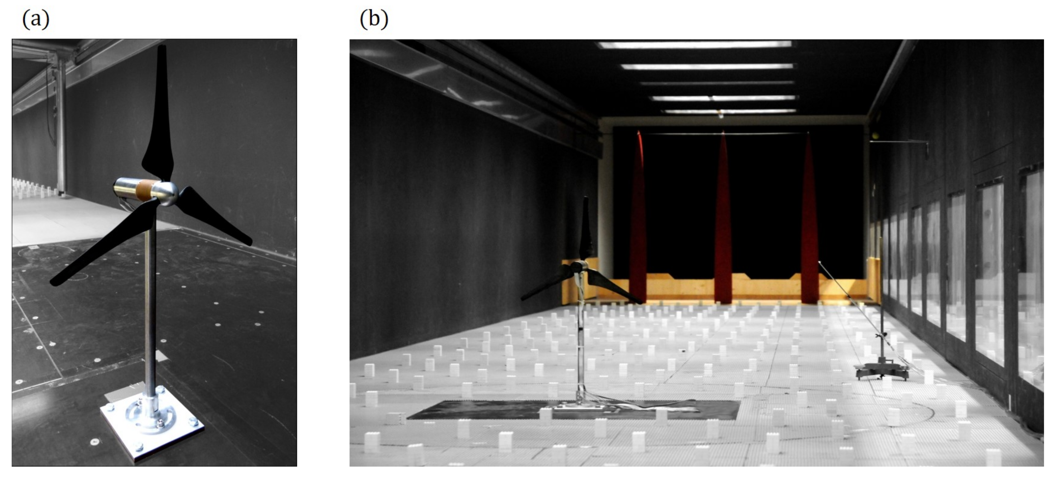
The rotor is mounted on a shaft which is supported by some additional bearings. The shaft is then connected via a clutch with a DC-generator. In order to extract the energy from the wind, the generator is actively loaded by a four-quadrant servo controller such that the wind turbine operates at an angular frequency $\mathsf{\Omega }$ which corresponds to the design tip-speed ratio of ${\lambda }_{dsgn}=\mathsf{\Omega }R/{\overline{u}}_{bl}\left(z_{hub}\right)=6.5$. Generator and nacelle are cylindrically shaped and have a diameter of 40 mm, whereas the tower, a circular cross-section tube, has a diameter of 20 mm. A strain gauge is installed between tower and nacelle to measure the axial forces on the rotor, nacelle and spinner. Simultaneously the electric current I produced by the generator is measured, from which the torque present at the rotor shaft $Q_{RS}$ can be calculated by the linear relation $Q_{RS}=kI$, where $k=99.4$ mNm/A is the torque constant of the motor. To obtain the mechanical torque at the rotor, $Q_{RS}$ is corrected for frictional losses in the bearings $Q_F\left({\lambda }_{dsgn}\right)=$ 9.14 mNm. The values k and $Q_F$ were determined by calibration using the torque meter rig developed by Bastankhah & Porté-Agel [34]. A photograph of the wind turbine model and the configuration of the boundary layer wind tunnel are shown in Figure 5.

4. Results

Before analysing the wake characteristics, the measured performance of the wind turbine immersed in both boundary layers is presented for varying tip-speed ratio and yaw angle. Afterwards the wake growth and its trajectory are discussed. Based on these values lateral profiles of the velocity deficit, the Reynolds shear stress and the turbulent kinetic energy are analysed regarding self-similarity as well as their scaling in the far wake region.

4.1. Rotor Performance

Performance measurements of the rotor within both turbulent boundary layers SBL and RBL are presented for tip-speed ratios $\lambda =$ 2.5–11.5 in un-yawed conditions and for the design tip-speed ratio of $\lambda =6.5$ for yaw angles $\gamma =0^{\circ }$–${45}^{\circ }$. As mentioned before, to avoid Reynolds number dependent effects, all measurements were performed at a chord based Reynolds number of $R{e}_c\approx$ 62,500, which is achieved by adapting the angular frequency $\mathsf{\Omega }$ and flow velocity at hub height $U_{hub}$ accordingly. Figure 6a,c show, for the mentioned range of tip-speed ratio, the variation of the power and thrust coefficients $C_P$ and $C_T$ which are defined as

$$C_P=\frac{Q\mathsf{\Omega }}{1/2\rho U_{hub}^3\pi R^2}\mathrm{and}{C}_T=\frac{T}{1/2\rho U_{hub}^2\pi R^2}.$$

(26)

Here Q and T are the torque and thrust produced by the rotor. As can be seen from Figure 6a,c, power and thrust curves differ slightly for the two boundary layers. Especially in case of the power coefficient, these differences vanish for tip-speed ratios $\lambda >7.5$. Power and thrust coefficient against yaw angle for a tip-speed ratio of ${\lambda }_{dsgn}=6.5$, normalised to their respective maximum value (un-yawed condition), are shown in Figure 6b,d. In this representation the curves exhibit an identical shape. Least squares fits of ${cos}^n\left(\gamma \right)$ with $n=2.5$ for the power and $n=1.5$ for the thrust coefficient fall for the design tip-speed ratio ${\lambda }_{dsgn}$ well in the range of other studies (e.g., [33,34,35]).

4.2. Wake Characteristics

Hot wire measurements in the wake of the wind turbine operating at the design tip-speed ratio ${\lambda }_{dsgn}$ were performed within the SBL and RBL boundary layer configuration for yaw angles of $\gamma =0^{\circ },{15}^{\circ },{30}^{\circ }$. Thereby the velocity field was recorded at downstream distances $x/R=2,4,6,10,14,18$ within the lateral range $-2.8<y/R<2.8$. For un-yawed conditions, the velocity field has also been recorded in the vertical plane for $0.47<z/R<3.63$ at the same downstream distances. The measured velocity profiles along the vertical coordinate in un-yawed conditions are shown in Figure 7a, whereas the measured velocity profiles along the lateral coordinate for un-yawed and yawed conditions are shown in Figure 7b,d. Just for the sake of clarity, the velocity profile at $x/R=4$ is left out in both figures. As already mentioned above, for the same yaw angles the wind turbine rotor produces similar thrust coefficients within both boundary layers. This results in an almost equal velocity deficit in the near wake ($x/R=2$) as can be seen in the figures. The far wake, however, clearly recovers faster for all yaw angles in the RBL compared to the SBL. This results from the higher background turbulence in case of the RBL, which enhances the momentum exchange between the wake and the outer flow. Due to that, in case of a yaw misalignment, the wake also looses its potential to penetrate the lateral undisturbed flow and is hence less deflected as it can be seen in Figure 7c,d. The lateral wake width ${\sigma }_y$ and wake center postion $y_C$ in the horizontal plane are derived from the measurements by numerical integration of the velocity deficit and momentum deficit respectively

$${\sigma }_y=\frac{1}{\sqrt{2\pi }max(\Delta u)}{\int }_{-\infty }^{\infty }\Delta udy\mathrm{and}{y}_C=\frac{{\int }_{-\infty }^{\infty }\Delta u^{2}ydy}{{\int }_{-\infty }^{\infty }\Delta u^{2}dy}.$$

(27)

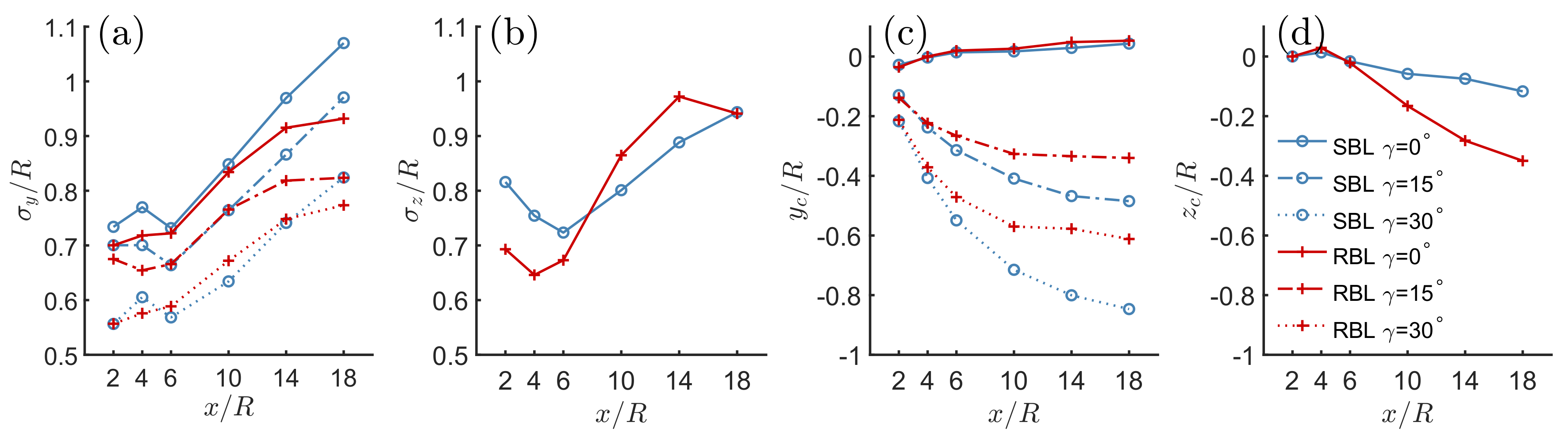
The vertical wake width ${\sigma }_z$ and wake center position $z_C$ are calculated analogously. The lateral wake width ${\sigma }_y$ as function of the axial position x is shown in Figure 8a for all measured yaw angles and flow conditions. Since measurements in the vertical plane only have been performed for unyawed conditions, the vertical wake width ${\sigma }_z$ is only calculated for these conditions and is shown in Figure 8b. In wind turbine wakes immersed in turbulent boundary layers a linear wake growth is often observed, where the lateral spreading rate is independent of the yaw angle, see e.g., [8]. This holds for the vertical and lateral wake width within the SBL for all measured yaw angles, where the lateral spreading rate $k_y=d{\sigma }_y/dx$ is nearly identical. It is also well known that the spreading rate increases with the level of turbulence (e.g., [36,37]). The measurements confirm this observation for the vertical wake width as shown in Figure 8b. However, in case of the lateral wake width, see Figure 8a, the spreading rate is slightly smaller within the RBL than in the SBL configuration. Furthermore, for downstream distances $x/R>10$ the spreading rates rather decrease than maintain a constant value. The lateral wake centreline position, determined by the momentum deficit Equation (27), is shown in Figure 8c for all measured cases. Vollmer & Steinfeld [3] observed in their LES study of a full scale wind turbine, immersed within a neutrally stratified boundary layer with a roughness comparable to the presented SBL, lateral wake deflections of similar magnitude.

As already mentioned before, due to the enhanced momentum transfer within the RBL, at yawed condition the wind turbine wake is significantly less deflected to the side compared to the SBL. There is also a noticeable displacement of the vertical centreline position towards the ground which is significantly increased in case of the RBL, see Figure 8d. This displacement as well as the deviations from the linear wake growth in case of the RBL can be explained with a loss of flow momentum in the wake of a wind turbine immersed in a highly sheared boundary layer as discussed in Section 2.1 and outlined in more detail in [4].

4.3. Self-Similarity

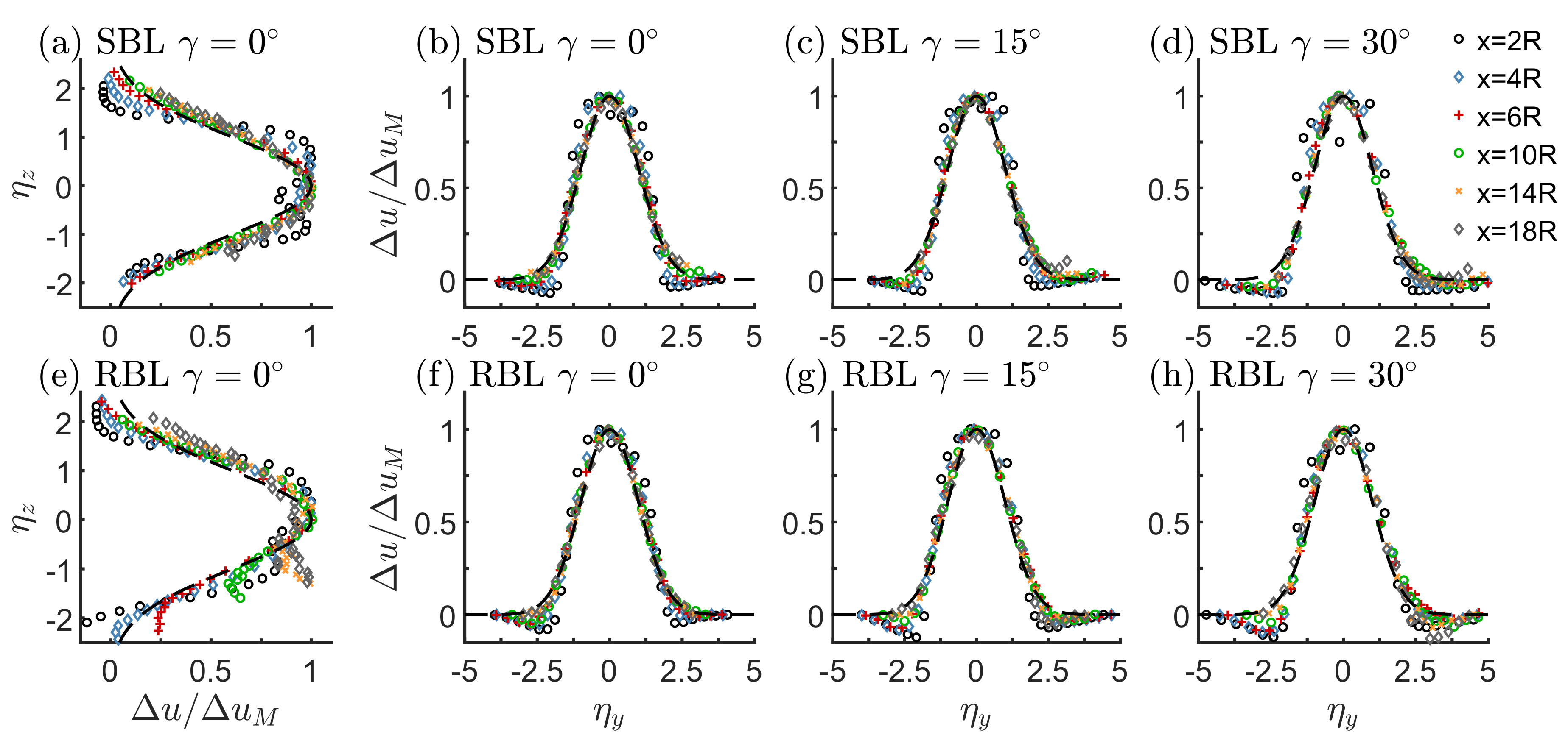
Together with the knowledge on the wake growth and the wake centreline position, the wind turbine wakes can now be analysed regarding their self-similarity. As starting point of this discussion, the profiles of the velocity deficit for all measured cases are shown in non-dimensional form in Figure 9. The profiles are therefore normalised by the maximum velocity deficit $\Delta u_M=max(\Delta u)$ at the respective downstream position. Furthermore, the lateral and vertical coordinate are shown in the non-dimensional form ${\eta }_y=(y-y_C)/{\sigma }_y$ and ${\eta }_z=(z-z_h)/{\sigma }_z$. As it is presumed that the vertical displacement observed in Figure 8d is rather biased by a loss of flow momentum than a real shift of the wake center, in the vertical direction the wake center is set equal to the hub height for all axial positions. As can be seen from Figure 9b–d,f–h for a sufficient axial distance from the rotor, all lateral profiles nearly collapse to a Gaussian distribution (shown as black dashed line) and therefore become self-similar. Within both boundary layers this state is reached within a distance of $x/R=6$ which in the following is considered to be the onset of the far wake.

In both boundary layers the profiles become slightly skewed with increasing yaw angle. Despite this fact, for the lateral profiles the degree of self-similarity can be considered as high across all measured yaw angles and boundary layer conditions. For the vertical profiles, shown in Figure 9a,e, the self-similarity can also be observed in case of the SBL, whereas in case of the RBL the normalized profiles are incomplete and do no longer collapse for vertical positions below hub height. This behaviour is considered to stem from the high mean velocity shear, which in this case is dominant enough to disturb the axial symmetry of the wake as well as the wake growth, see above in Section 4.2. As a result, the concept of decomposition of the flow in a boundary layer and a wake does not longer seem to be appropriate in this region.

Having shown the self-similarity of the axial mean velocity component in the wake of the model wind turbine for various yaw angles and boundary layer conditions, one is tempted to determine the underlying scaling law for the centreline velocity deficit $\Delta u_C$ and the vertical and lateral half width ${\sigma }_z$ and ${\sigma }_y$ by fitting Equations (18) and (19) to the measurement data. However, Obligado et al. [24], showed that optimal coefficients A, B and virtual origins $x_{0u}$, $x_{0\sigma }$ can be found that give a reasonable fit to the measurement data within a certain range of values for the exponents $n_u$, $n_{\sigma }$. They therefore concluded that it is impossible to discriminate between equilibrium and non-equilibrium scaling by only fitting the centreline velocity deficit and wake width data. To probe this statement, we performed a simple linear regression regarding the scaling laws discussed in Section 2.2 which results in a similar finding. As the wake growth is significantly different within the near wake $x/R<6$, and in case of the RBL configuration also for $x/R\ge 14$, these data points are not used in the fitting procedure. Figure 10 shows the resulting fits in a linear representation, where in (a)–(c) the lateral wake widths and (d)–(f) the centreline velocity deficits are shown. In this representation the resulting fits to different scaling laws are almost indistinguishable by eye, just the fit to the equilibrium scaling law of the velocity deficit in Figure 10d does not cope with the measurements. Thus, in order to arrive at a distinct conclusion on the appropriate scaling law, it is highly desirable to get an independent assessment by analysing the evolution of the added Reynolds shear stress and the added turbulent kinetic energy.

As the equilibrium and non-equilibrium scaling laws only predict the self-similarity of the Reynolds shear stress and the turbulent kinetic energy, and not of their added equivalent, the self-similarity of these quantities has first to be established. We therefore test for it by normalising the profiles by the x-dependent profile’s maximum as it is done above for the velocity deficit. For the added Reynolds shear stress $\Delta \overline{u^{\prime }{u}_r^{\prime }}$ this is shown in the vertical and horizontal plane of all measured cases in Figure 11. The respective maximum values $\Delta {\overline{u^{\prime }{u}_r^{\prime }}}_M=max\left(\right|\Delta \overline{u^{\prime }{u}_r^{\prime }}\left|\right)$ are shown in Figure 14a. The vertical and lateral coordinate is thereby again represented by ${\eta }_z=(z-z_h)/{\sigma }_z$ and ${\eta }_y=(y-y_C)/{\sigma }_y$, respectively. In the lateral direction, see Figure 11b–d for the SBL and Figure 11f–h for the RBL, it can be seen that all profiles nearly collapse to a single curve, even at high yaw angles. Only in case of the RBL with the wind turbine operating at a yaw angle of $\gamma ={30}^{\circ }$ more significant deviations can be observed. The self-similar profiles approximately follow a distribution of $-\eta e^{-0.5({\eta }^2-1)}$ shown in the Figures as black dashed line. As it was already observed for the velocity deficit, the vertical mean wind shear also prevents the vertical profiles of the added Reynolds shear stress to collapse in the region below the hub. Therefore, the profiles are normalised by the maximum value of the added shear stress which occurs above the hub height $\Delta {\overline{u^{\prime }{u}_r^{\prime }}}_M=max\left(\right|\Delta \overline{u^{\prime }{u}_r^{\prime }}(z>z_{hub}|)$ as only here self-similarity can be expected. In the region above the hub and for downstream distances $x/R\ge 10$, the profiles nearly collapse to the same distribution as it is observed in the horizontal plane. Below the hub the profiles however differ significantly, especially in the case of the RBL.

Figure 12 shows the vertical and horizontal profiles of the added turbulent kinetic energy in self-similar form. The respective maximum values $\Delta K_M$, used for normalising the profiles, are given in Figure 14e. For the vertical profiles of the added turbulent kinetic energy, shown in Figure 12a,e, self-similarity can just be observed in the region above the hub and for downstream distances $x/R\ge 10$. In the horizontal plane, however, other than in the case of the added shear stress, the degree of self-similarity differs significantly between both boundary layers, as it can be seen in Figure 12b–d for the SBL and in Figure 12f–h for the RBL. In case of the SBL, the profiles become self-similar for downstream distances $x/R\ge 10$ whereby they also become slightly skewed with increasing yaw angle. For the cases within the RBL, however, the profiles just exhibit a low degree of self-similarity, especially for yawed conditions. In these cases, the side of the profiles toward which the wake is deflected ( ${\eta }_y<0$ ) does not collapse onto a single curve whereas the opposite side does. It is important to note that neither the equilibrium nor the non-equilibrium theory explicitly predicts the self-similarity of the diagonal components of the added Reynolds stress tensor. However, motivated by the observed self-similarity of the added turbulent kinetic energy in case of the SBL flow, these quantities are also shown in self-similar form for this flow condition in Figure 13. It can be observed that all three quantities exhibit a similar degree of self-similarity as the added turbulent kinetic energy does. Additionally, the Gaussian distributions, shown as black dashed lines, are obtained by a least square curve fit to the added Reynolds stresses measured in the horizontal plane for a yaw angle of $\gamma =0^{\circ }$. With that it becomes clear that with increasing yaw angle the profiles of the added Reynolds stresses $\overline{u^{\prime }{u}^{\prime }}$ and $\overline{w^{\prime }{w}^{\prime }}$ become asymmetric regarding the wake centreline while the component in the lateral direction $\overline{v^{\prime }{v}^{\prime }}$ stays almost symmetric. Despite the increasing asymmetry all profiles maintain their degree of self-similarity.

Having confirmed the existence of self-similarity for the added components $\Delta \overline{u^{\prime }{u}_r^{\prime }}$ and $\Delta \overline{u_i^{\prime }{u}_i^{\prime }}$ of the Reynolds stress tensor and the added turbulent kinetic energy $\Delta K$, the x-dependency of the underlying scaling of these quantities can now be analysed in detail. Therefore, Figure 14b–d assesses the validity of the three scalings stated in Equation (25) for the added Reynolds shear stress and in Figure 14f–h for the added turbulent kinetic energy.

Whereas in (b)/(f) the equilibrium scaling law is used, in (c)/(g) the square-root wake growth scaling law and in (d)/(h) the linear wake growth scaling law is applied. For the sake of clarity, the ratios are additionally normalised by their respective value at $x/R=6$, as this location is considered as the onset of the far wake. In this representation it becomes clear that neither the equilibrium nor the square-root wake growth scaling law reproduces the x-dependence of the added Reynolds shear stress and the added turbulent kinetic energy in the wake of the model wind turbine correctly. However, the linear wake growth scaling normalises both quantities to an approximately constant value which suggests a scaling of $\Delta {\overline{u^{\prime }{u}_r^{\prime }}}_M,\Delta K_M\propto \Delta u_C\propto x^{-2}$. An important consequence from these findings is that only a member of the non-equilibrium scaling laws, namely the linear wake growth scaling, can form a base for a consistent scaling of all fundamental wind turbine wake parameters, including the velocity deficit, wake width, and maxima for all components of the Reynolds stress tensor. This finding is one of the main results of the present study and might be helpful in assessing the predictive capability of wake models as done in [4].

Due to the high degree of self-similarity observed also for the added Reynolds stresses $\Delta \overline{u_i^{\prime }{u}_i^{\prime }}$, naturally the question arises how these quantities scale in the axial direction. As mentioned in Section 2.3, Dairay et al. [18] argue that non-equilibrium flows in which $n=m\ne 1$ should only be possible under the assumption of a constant anisotropy on the surface $\eta =1$. For that reason the ratio $(\Delta \overline{u_i^{\prime }{u}_i^{\prime }}/\Delta K)(\eta =1)$ is shown in Figure 15a–c along the line ${\eta }_z=1$ and in (e)–(g) along the line ${\eta }_y=1$. On the line ${\eta }_z=1$ the ratio $(\Delta \overline{u_i^{\prime }{u}_i^{\prime }}/\Delta K)({\eta }_z=1)$ is almost equal for both boundary layers and converges clearly to constant values as it is postulated by Dairay. However, on the line ${\eta }_y=1$ the ratio differs for both boundary layers. Nevertheless, for the SBL the ratio also clearly converges towards values which just vary by about 5% from the values at ${\eta }_z=1$ and are similar even at large yaw angles. Within the RBL the ratios differ by about 30% from their counterpart within the SBL. Also for yawed conditions the curves deviate more, yet without any clear trend. These deviations can be explained by the lower degree of self-similarity of the added turbulent kinetic energy in case of the RBL, which for increasing yaw angles is subsequently perturbed, see Figure 12.

Nevertheless, the significant differences between both boundary layers for the ratio $\Delta K({\eta }_y=1)/\Delta u_C$, shown in Figure 15h, are not likely to result from a deviation of the self-similarity as they just exhibit a slight dependency on the yaw angle. The difference is rather assumed to result from the different level of background turbulence. This is also consistent with the almost similar ratios $\Delta K({\eta }_z=1)/\Delta u_C$, shown in Figure 15d, since the difference in background turbulence at this height vanishes. In the introduction of this work, see Section 1, we addressed the variety of scaling exponents found in literature for the added turbulence intensity $I_{+}$. As we have shown that the linear wake growth scaling correctly predicts a scaling of $\Delta K_M\propto \Delta u_C\propto x^{-2}$, the observation of (i) self-similarity of the diagonal components of the added Reynolds stress tensor and (ii) an approximately constant anisotropy consequently suggests a physically motivated scaling of $I_{+}=\sqrt{\Delta \overline{u^{\prime }{u}^{\prime }}}\propto x^{-1}$.

5. A Simple Analytical Model for Turbulence Quantities in the Far Wake Region

The model is based on the assumption that the diagonal components of the Reynolds stress tensor $\overline{u_i^{\prime }{u}_i^{\prime }}$ and the turbulent kinetic energy K in the wake can be expressed in terms of the added quantities $\Delta \overline{u_i^{\prime }{u}_i^{\prime }}$ and $\Delta K$

$$\frac{\overline{u_i^{\prime }{u}_i^{\prime }}(x,y,z)}{{\overline{u}}_{bl}^2\left(z\right)}=\frac{{\overline{u_i^{\prime }{u}_i^{\prime }}}_{bl}(z,I_0)}{{\overline{u}}_{bl}^2\left(z\right)}+\Delta \overline{u_i^{\prime }{u}_i^{\prime }}(x,y,z,C_T,\gamma ,I_0),\frac{K(x,y,z)}{{\overline{u}}_{bl}^2\left(z\right)}=\frac{K_{bl}(z,I_0)}{{\overline{u}}_{bl}^2\left(z\right)}+\Delta K(x,y,z,C_T,\gamma ,I_0)$$

(28)

where $I_0$ shall indicate the dependency on the level of background turbulence, which here is not further defined. In the following we subsequently make use of the findings in Section 4.3 to meet reasonable assumptions. It was found that the diagonal components of the added Reynolds stress tensor $\Delta \overline{u_i^{\prime }{u}_i^{\prime }}$ and the added turbulent kinetic energy exhibit a high degree of self-similarity in the wake. Therefore, we assume that these quantities can be approximated by

$$\Delta \overline{u_i^{\prime }{u}_i^{\prime }}=\Delta \overline{u_i^{\prime }{u}_i^{\prime }}(\eta =1)·f_{ii}\left(\eta \right),\Delta K=\Delta K(\eta =1)·h\left(\eta \right).$$

(29)

Furthermore, the results shown in Figure 15 suggest a constant anisotropy in the far wake region $\Delta \overline{u_i^{\prime }{u}_i^{\prime }}\propto \Delta K$, as well as the axial scaling $\Delta K_M\propto \Delta u_C$ that was identified in Figure 14 and which governs the streamwise evolution of the magnitude of the stresses. Hence, we define the constants $C_i=\Delta \overline{u_i^{\prime }{u}_i^{\prime }}(\eta =1)/\Delta K(\eta =1)$ and $C_K\left(I_0\right)=\Delta K(\eta =1)/\Delta u_C$ which can readily be taken from Figure 15 (note the condition $0.5\sum C_i=1$). Inserting these into Equation (28) then gives

$$\frac{\overline{u_i^{\prime }{u}_i^{\prime }}}{{\overline{u}}_{bl}^2}=\frac{{\overline{u_i^{\prime }{u}_i^{\prime }}}_{bl}}{{\overline{u}}_{bl}^2}+C_i·C_K\left(I_0\right)·\Delta u_C(x,C_T,\gamma )·f_{ii}\left(\eta \right),\frac{K}{{\overline{u}}_{bl}^2}=\frac{K_{bl}}{{\overline{u}}_{bl}^2}+C_K\left(I_0\right)·\Delta u_C(x,C_T,\gamma )·h\left(\eta \right).$$

(30)

The shape functions $f_{ii}$, however, have to be determined from the measurements. It is likely that these, as well as the constants $C_i$ and $C_K$, might depend on the rotor design and could also vary with operational parameters as the tip-speed ratio. Therefore it should be noted that, as mentioned in Section 3.3, the rotor is designed for constant bound circulation and is operated at its optimum tip-speed ratio in terms of power production. The slight asymmetry of the shape functions, see Figure 13, in yawed conditions is here neglected. With that the shape functions can be approximated by

$$f_{11}=exp[-{\alpha }_1{(\eta -1)}^2]+exp[-{\alpha }_1{(\eta +1)}^2],f_{22,33}=exp\left[{\alpha }_{2,3}(1-{\eta }^2)\right]$$

(31)

and are all formulated such that $f_{ii}\left(\right|\eta |=1)=1$. Since $\Delta K=0.5\sum \Delta \overline{u_i^{\prime }{u}_i^{\prime }}$, the shape function of the turbulent kinetic energy can simply formulated as

$$h\left(\eta \right)=0.5\sum C_i{f}_{ii}\left(\eta \right).$$

(32)

Parameters which are derived from the mean velocity field, as $\Delta u_C$, $y_C$ and ${\sigma }_y$, can be computed from any appropriate analytical wake model (base model) which predicts the velocity distribution in the wake. A comparison of two analytical wake models against the measurement data presented here can be found in [4]. However, for testing purposes we derive these parameters directly from the measurements in order not to introduce any errors from modelling assumptions on the velocity field. For the aforementioned test we determine all necessary parameters on the basis of the results in the horizontal plane at hub height for the unyawed turbine which result in ${\alpha }_1=1.25$, ${\alpha }_2=0.35$, ${\alpha }_3=0.28$, $C_1=0.8$, $C_2=0.6$ and $C_3=0.6$. The constants $C_K$ are calculated as the average value at the last three axial measurement stations which gives $C_K\left(SBL\right)=0.049$ and $C_K\left(RBL\right)=0.030$. As shown in Figure 16, the model predictions and measurements gradually converge. For large yaw angles the neglected asymmetry of the shape functions becomes noticeable, especially in case of the RBL. However, as intentional large yaw angles are rather impractical for wake control strategies, due to the substantial decrease of the power coefficient, this might be a rather less important inaccuracy of the model. Since typical turbine spacings in windfarms are in the range covered by this simple model, it might be useful within the context of real time wake control strategies when coupled to a suitable base model for $\Delta u_C$, $y_C$ and ${\sigma }_y$.

6. Summary and Conclusions

Wind tunnel measurements of a wind turbine immersed in two neutrally stratified turbulent boundary layers of different aerodynamic roughness and operating at various yaw angles $\gamma$ were presented. Measurements of generated power and thrust were carried out to analyse the performance of the turbine under these conditions. Yaw-angle dependencies of the power $C_P$ and thrust coefficient $C_T$ are shown to be insensitive to changes in shear and turbulence intensity. It was found that $C_P$ and $C_T$ decrease with increasing yaw angle, following a $cos{\left(\gamma \right)}^n$-distribution. For the design tip-speed ratio the exponents n are similar to values reported in the literature. Within both boundary layers hot wire measurements were conducted in the wake of the model wind turbine for each yaw angle. It is found that with increasing turbulence intensity (and shear) of the boundary layer (i) the wake recovers faster due to an enhanced mixing of the wake and the outer flow, and (ii) the wake is less deflected under yawed conditions.

Analytical considerations show that a superposition of a turbulent boundary layer and a wind turbine wake is a useful approximative description of the flow. The approach, however, is constrained (i) to regions where far wake assumptions are valid but wake quantities are still significant enough and (ii) to turbulent boundary layers with moderate velocity shear. Wake measurements in a moderately sheared boundary layer confirm the accuracy of this approach for the mean axial velocity, the Reynolds shear stress and the turbulent kinetic energy. On the other hand, measurements within a highly sheared boundary layer show the limitations of this approach. It is found that if described in terms of an added quantity, lateral and vertical profiles of the mean axial velocity, the Reynolds shear stress and the turbulent kinetic energy become self-similar in the far wake, even at high yaw angles.

Due to the high degree of self-similarity, the wake is analysed regarding the underlying scaling law of the velocity deficit, the wake growth, the added Reynolds shear stress and the added turbulent kinetic energy. It is shown that the streamwise scaling of the velocity deficit and the wake growth cannot be clearly identified by fitting the centreline velocity deficit and the wake width data. Analysis of the added Reynolds shear stress and the added turbulent kinetic energy reveal that the maxima of these quantities scale proportional to the centreline velocity deficit $\Delta {\overline{u^{\prime }{u}_r^{\prime }}}_M,\Delta K_M\propto \Delta u_C$. This is consistent with the non-equilibrium scaling Equation (22) which predicts ${\overline{u^{\prime }{u}_r^{\prime }}}_M\propto K_M$ [18] and allows a proportionality to the centreline velocity deficit $\Delta u_C$ if the exponents m, n are chosen to be $m=n=2$. In this case the non-equilibrium scaling also predicts a linear wake growth, as it is observed in the presented results for the wind turbine immersed within a boundary layer with smooth ground roughness as well as in other corresponding studies. In the rough boundary layer, the wake width does not strictly follow a linear growth rate despite convincing self-similarity of mean flow and Reynolds stress profiles. Since other wake parameters develop according to the non-equilibrium scaling law, we believe that the proposed scaling concept is applicable to a wide range of ambient conditions. To the authors’ knowledge, it is the first time that the non-equilibrium scaling theory is applied to the wake of a wind turbine immersed in a turbulent boundary layer. Moreover, the anisotropy of the added Reynolds stresses is considered along the non-dimensional coordinate $\eta =1$ and found to be approximately constant within the far wake region, whereas the contributions of the added Reynolds stresses slightly change with increasing background turbulence. The ratio $C_K=\Delta K(\eta =1)/\Delta u_C$, however, is significantly influenced by the level of background turbulence and further research is necessary to determine its value for various flow and operational conditions. Given an approximately constant anisotropy, a self-similarity of the diagonal components of the added Reynolds stress tensor and the validity of the linear wake growth scaling $\Delta K_M\propto \Delta u_C$, the results suggest a physically motivated scaling of $I_{+}=\sqrt{\Delta \overline{u^{\prime }{u}^{\prime }}}\propto x^{-1}$.

Based on these findings a simple model to predict the diagonal components of the Reynolds stress tensor is proposed. It applies to steady ambient conditions and fixed operational parameters. Due to its formulation, it can be used as extension to existing analytical wake models which predict the flow field in the wake and needs only $C_K\left(I_0\right)=\Delta K(\eta =1)/\Delta u_C$ as additional input parameter. A comparison of the measurements in the horizontal plane of the rotor is in good agreement with the predicted Reynolds stresses and turbulent kinetic energy. Nevertheless, for a generalisation of the model, in future studies the dependencies of the parameter $C_K\left(I_0\right)$, $C_i$ and the shape functions $f_{ii}$ on the ambient conditions and on the operational state of the wind turbine have to be analysed in detail. Since the study is based on the analysis of a single wake, additional research effort is necessary for extending the model to predict the evolution of turbulence within multiple interacting wakes. With such an extension, the model could be applied in real-time wind farm controllers for the optimization of power production and alleviation of fatigue loads.

References

- Knudsen, T.; Bak, T.; Svenstrup, M. Survey of wind farm control—Power and fatigue optimization. Wind Energy 2015, 18, 1333–1351. [Google Scholar] [CrossRef]
- Abkar, M.; Porté-Agel, F. Influence of atmospheric stability on wind-turbine wakes: A large-eddy simulation study. Phys. Fluids 2015, 27, 035104. [Google Scholar] [CrossRef] [Green Version]
- Vollmer, L.; Steinfeld, G. Estimating the wake deflection downstream of a wind turbine in different atmospheric stabilities: An LES study. Wind Energy Sci. 2016, 1, 129–141. [Google Scholar] [CrossRef]
- Stein, V.P.; Kaltenbach, H.J. Influence of ground roughness on the wake of a yawed wind turbine—A comparison of wind-tunnel measurements and model predictions. J. Phys. Conf. Ser. 2018, 1037, 072005. [Google Scholar] [CrossRef]
- Xie, S.; Archer, C. Self-similarity and turbulence characteristics of wind turbine wakes via large-eddy simulation. Wind Energy 2015, 18, 1815–1838. [Google Scholar] [CrossRef]
- Katic, I.; Højstrup, J.; Jensen, N. A simple model for cluster efficiency. In EWEA Conference; A. Raguzzi: Rome, Italy, 1986; pp. 407–410. [Google Scholar]
- Larsen, G.C. A Simple Wake Calculation Procedure; Risø-M 2760; DTU: Lyngby, Denmark, 1988; Volume 15. [Google Scholar]
- Bastankhah, M.; Porté-Agel, F. Experimental and theoretical study of wind turbine wakes in yawed conditions. J. Fluid Mech. 2016, 806, 506–541. [Google Scholar] [CrossRef]
- Quarton, D.C. Wake Turbulence Characterisation; Final Report from Garrad Hassan and Partners to the Energy Technology Support Unit of the Department of Energy of the UK; Contract No. ETSUWN 5096; Department of Energy: London, UK, 1989. [Google Scholar]
- Crespo, A.; Hernández, J. Turbulence characteristics in wind-turbine wakes. J. Wind Eng. Ind. Aerod. 1996, 61, 71–85. [Google Scholar] [CrossRef]
- Frandsen, A. Turbulence and Turbulence Generated Structural Loading in Wind Turbine Clusters. Ph.D. Thesis, RisøNational Laboratory, Roskilde, Denmark, 2007. [Google Scholar]
- Chamorro, L.P.; Porté-Agel, F. A Wind-Tunnel Investigation of Wind-Turbine Wakes: Boundary-Layer Turbulence Effects. Bound.-Layer Meteorol. 2009, 132, 129–149. [Google Scholar] [CrossRef] [Green Version]
- George, W.K.; Arndt, R. The self-preservation of turbulent flows and its relation to initial conditions and coherent structures. Adv. Turbul. 1989, 39–73. [Google Scholar]
- Seoud, R.E.; Vassilicos, J.C. Dissipation and decay of fractal-generated turbulence. Phys. Fluids 2007, 19, 105108. [Google Scholar] [CrossRef] [Green Version]
- Mazellier, N.; Vassilicos, J.C. Turbulence without Richardson-Kolmogorov cascade. Phys. Fluids 2010, 22, 075101. [Google Scholar] [CrossRef]
- Nagata, K.; Sakai, Y.; Inaba, T.; Suzuki, H.; Terashima, O.; Suzuki, H. Turbulence structure and turbulence kinetic energy transport in multiscale/fractal-generated turbulence. Phys. Fluids 2013, 25, 065102. [Google Scholar] [CrossRef]
- Nedic, J.; Vassilicos, J.C.; Ganapathisubramani, B. Axisymmetric turbulent wakes with new non-equilibrium similarity scalings. Phys. Rev. Lett. 2013, 111, 144503. [Google Scholar] [CrossRef] [PubMed]
- Dairay, T.; Obligado, M.; Vassilicos, J.C. Non-equilibrium scaling laws in axisymmetric turbulent wakes. J. Fluid Mech. 2015, 781, 166–195. [Google Scholar] [CrossRef] [Green Version]
- Vassilicos, J.C. From Tennekes and Lumley to Townsend and to George: A Slow March to Freedom. In Whither Turbulence and Big Data in the 21st Century? Pollard, A., Castillo, L., Danaila, L., Glauser, M., Eds.; Springer: Cham, Switzerland, 2017; pp. 3–11. [Google Scholar]
- Pope, S.B. Turbulent Flows; Cambridge University Press: Cambridge, UK, 2000. [Google Scholar]
- Carmody, T. Establishment of the wake behind a disk. J. Basic Eng. 1964, 86, 869. [Google Scholar] [CrossRef]
- Johansson, P.B.; George, W.K. Equilibrium similarity, effects of initial conditions and local Reynolds number on the axisymmetric wake. Phys. Fluids 2003, 15, 603–617. [Google Scholar] [CrossRef] [Green Version]
- Uberoi, M.S.; Freymuth, P. Turbulent Energy Balance and Spectra of the Axisymmetric Wake. Phys. Fluids 1970, 13, 2205–2210. [Google Scholar] [CrossRef]
- Obligado, M.; Dairay, T.; Vassilicos, J.C. Nonequilibrium scalings of turbulent wakes. Phys. Rev. Fluids 2016, 1, 044409. [Google Scholar] [CrossRef] [Green Version]
- Valente, P.C.; Vassilicos, J.C. Universal Dissipation Scaling for Nonequilibrium Turbulence. Phys. Rev. Lett. 2012, 108, 214503. [Google Scholar] [CrossRef] [PubMed]
- Vassilicos, J.C. Dissipation in Turbulent Flows. Annu. Rev. Fluid Mech. 2015, 47, 95–114. [Google Scholar] [CrossRef] [Green Version]
- Counihan, J. An improved method of simulating an atmospheric boundary layer in a wind tunnel. Atmos. Environ. 1969, 3, 197–214. [Google Scholar] [CrossRef]
- Breitsamter, C. Turbulente Strömungsstrukturen an Flugzeugkonfigurationen mit Vorderkantenwirbeln. Ph.D. Thesis, TUM, Munich, Germany, 1997. [Google Scholar]
- Counihan, J. Adiabatic atmospheric boundary layers: A review and analysis of data from the period 1880–1972. Atmos. Environ. 1975, 9, 871–905. [Google Scholar] [CrossRef]
- Heist, D.K.; Castro, I.P. Combined laser-doppler and cold wire anemometry for turbulent heat flux measurement. Exp. Fluids 1998, 24, 375–381. [Google Scholar] [CrossRef]
- Chamorro, L.P.; Arndt, R.E.A.; Sotiropoulos, F. Reynolds number dependence of turbulence statistics in the wake of wind turbines. Wind Energy 2012, 15, 733–742. [Google Scholar] [CrossRef]
- Selig, M.; Donovan, J.; Frase, D. Airfoils at Low Speeds; H.A. Stokely: Virginia Beach, VA, USA, 1989. [Google Scholar]
- Burton, T.; Jenkins, N.; Sharpe, D.; Bossanyi, E. Wind Energy Handbook; John Wiley & Sons: Chichester, UK, 2011; ISBN 978-0-470-69975-1. [Google Scholar]
- Bastankhah, M.; Porté-Agel, F. A New Miniature Wind Turbine for Wind Tunnel Experiments. Part I: Design and Performance. Energies 2017, 10, 908. [Google Scholar] [CrossRef]
- Krogstad, P.; Adaramola, M. Performance and near wake measurements of a model horizontal axis wind turbine. Wind Energy 2012, 15, 743–756. [Google Scholar] [CrossRef]
- Wu, Y.; Porté-Agel, F. Atmospheric Turbulence Effects on Wind-Turbine Wakes: An LES Study. Energies 2012, 5, 5340–5362. [Google Scholar] [CrossRef]
- Jin, Y.; Chamorro, L. Effects of Freestream Turbulence in a Model Wind Turbine Wake. Energies 2016, 9, 830. [Google Scholar] [CrossRef]
Figure 1.
Sketch of the two superimposed flow fields.
Figure 2.
(a) Mean axial velocity , (b) axial Reynolds stress component , (c) shear stress and (d) longitudinal integral length scale within the turbulent boundary layer. All quantities are normalised by the mean velocity at hub height and the rotor radius R. The rotor edges are indicated by horizontal dashed lines and the legend denotes the flow conditions.
Figure 3.
(a) Normalised energy spectral density of the axial velocity component within the boundary layers. Pre-multiplied normalised energy spectral density in the wake of the wind turbine at (b) and (c) , all measured at hub height . The legend denotes flow conditions, dashed lines denote the slope of the Kolmogorov cascade.
Figure 4.
(a) Chord and (b) Twist distribution. Dashed line represents Burton’s optimum distribution and solid line is the modified distribution.
Figure 5.
(a) Model Wind Turbine and (b) Model Wind Turbine within the boundary layer wind tunnel with roughness elements and barriers for the SBL configuration.
Figure 6.
(a,c) Power and (b,d) thrust coefficients and as function of tip-speed ratio and yaw angle for constant chord based Reynolds number 62,500. The legend states the flow conditions. For the coloured points hot wire measurements were performed.
Figure 7.
(a) Vertical and (b–d) horizontal profiles of the normalised streamwise velocity in the wake of the model wind turbine immersed within the SBL (blue line) and RBL (red line) operating at (a)/(b) , (c) and (d) . Horizontal dashed lines indicate the rotor edges.
Figure 8.
(a) Lateral and (b) vertical wake half widths and , (c) lateral and (d) vertical wake deflections and as function of the axial distance . The legend indicates flow condition and yaw angle for both subfigures.
Figure 9.
Vertical and lateral profiles of the normalised velocity deficit versus and in the wake of the model wind turbine immersed in the SBL with (a)/(b) , (c) , (d) and in the RBL with (e)/(f) , (g) , (h) . The black dashed line denotes a Gaussian distribution . The legend indicates the downstream position.
Figure 10.
Normalised lateral wake width and normalised centreline velocity deficit as function of for (a)/(d) the equilibrium scaling ; for (b)/(e) the square-root wake growth scaling ; for (c)/(f) the linear wake growth scaling . Fits include the range for SBL and for RBL. The legend indicates the flow conditions.
Figure 11.
Vertical and lateral profiles of the normalised added Reynolds shear stress versus and in the wake of the model wind turbine immersed in the SBL with (a)/(b) , (c) , (d) and in the RBL with (e)/(f) , (g) , (h) . Black dashed line denotes the distribution . The legend indicates the downstream position.
Figure 12.
Vertical and lateral profiles of the normalised added turbulent kinetic energy versus and in the wake of the model wind turbine immersed in the SBL with (a)/(b) , (c) , (d) and in the RBL with (e)/(f) , (g) , (h) . The legend indicates the downstream position.
Figure 13.
Vertical and lateral profiles of the normalised diagonal components of the added Reynolds stress tensor versus and in the wake of the model wind turbine immersed in the SBL. Black dashed line denotes the distributions (b)–(d) , (f)–(h) and (j)–(l) . The legend indicates the downstream position.
Figure 14.
(a) Maximum added Reynolds shear stress and (e) maximum added turbulent kinetic energy in the wake of the model wind turbine, measured in the horizontal (hp) and vertical plane (vp), normalised using (b)/(f) equilibrium scaling , (c)/(g) square-root wake growth scaling , (d)/(h) linear wake growth scaling . The legend indicates the flow and yaw conditions.
Figure 15.
Structural parameters and in the wake of the model wind turbine for (a)–(d) and (e)–(h) . The legend gives flow and yaw conditions.
Figure 16.
Comparison of model predictions (lines) and measurement results (symbols and lines) in the horizontal plane at hub height for the Reynolds stress components (a) , (b) and (c) , and (d) the turbulent kinetic energy K, all normalised by . The legend gives flow conditions.