Changing the Day-Ahead Gate Closure to Wind Power Integration: A Simulation-Based Study

Abstract

Currently, in most European electricity markets, power bids are based on forecasts performed 12 to 36 hours ahead. Actual wind power forecast systems still lead to large errors, which may strongly impact electricity market outcomes. Accordingly, this article analyzes the impact of the wind power forecast uncertainty and the change of the day-ahead market gate closure on both the market-clearing prices and the outcomes of the balancing market. To this end, it presents a simulation-based study conducted with the help of an agent-based tool, called MATREM. The results support the following conclusion: a change in the gate closure to a time closer to real-time operation is beneficial to market participants and the energy system generally.

1. Introduction

Electricity market (EMs) are a complex and continuously evolving reality—new players are emerging and new strategic behaviors are gaining more active roles, meaning that researchers and practitioners did not yet solve the problems associated with this new reality [1,2]. Chief among these problems are the ones related to the increase in non-dispatchable renewable generation, or variable renewable energy (VRE), such as solar and wind power. VRE is characterized by substantial investment costs, but near-zero marginal costs, and great variability, thus increasing the uncertainty of the net load. VRE is normally the marginal resource, since it is operated at maximum capacity (taking into account the weather conditions). These characteristics have a strong influence on the outcomes of energy markets, reducing market-clearing prices [3]. Accordingly, existing market designs should be analyzed to determine if they are still efficient to deal with high levels of VRE (see, e.g., [4,5,6]).

The question of a suitable day ahead market design for a better integration of VRE has been the subject of a great deal of research (see, e.g., [7,8,9,10]). For the particular case of an effective gate closure, the potential solution discussed by the research community involves its adjustment to a time closer to the first hour of delivery. The main reason behind this adjustment is related to the forecast of renewable generation, which typically presents large errors for long time horizons, due to the stochastic nature of the atmosphere. Since the day-ahead market (DAM) closes typically at 12:00 p.m. (CET), the bids of wind power producers need to be performed through power forecasts computed at least 12 to 36 h ahead. Consequently, the adjustment of the gate closure is very important to enable a fair participation of VRE in EMs, since all energy producers (dispatchable and non-dispatachable) participate in the day-ahead market under the same rules. In case the energy production differs from the commitments resulting from the DAM, the differences should be balanced in the intraday market and/or the balancing market.

In 2014, the International Agency of Energy (IEA) presented a report about energy markets and renewable generation [11], scoring key EM features according to eight dimensions: non-VRE dispatch, VRE dispatch, dispatch interval, last schedule update, grid representation, interconnector management and system services definition and market. Half of these dimensions are directly related to the improvement of forecasts, namely dispatch interval, grid representation, interconnector management and last schedule update. IEA considers that all physical transactions should be performed through implicit auctions in a centralized pool without feed-in-tariffs (FiTs) or other incentives to renewable energy sources (RES), with an interval up to 10 min using updates up to 30 min before real-time operation. In addition, the reserve requirements should be computed stochastically, taking into account different scenarios for the share of VRE, and be remunerated through marginal pricing. Furthermore, dispatch intervals should be reduced—that is, should be as short as possible—to enable VRE producers to perform high accurate forecasts. Such market modifications can contribute to a new paradigm—a paradigm of VRE integration without FiTs, where VRE investors do not have a guaranteed return, being remunerated by the market price, and subject to the payment of penalties for their deviations.

In 2016, the European Union (EU) presented the “Clean Energy for all Europeans”, a package of measures to promote the integration of renewable generation and to harmonize the European markets. In 2017, the EU presented a new proposal for regulating the pan-European market [12]. Article 7 considers that market operators should trade as close as possible to real-time operation, and no later than the gate closure of the intraday cross-zonal market. In [13], we presented an overview of the potential effects of the new EU proposal on the integration of renewable generation. In [14,15,16], we analyzed the impact of both high levels of renewable generation and significant forecast errors on the outcomes of the DAM. As a preliminary result, we conclude that a gate-closure closer to real time operation is beneficial to wind power producers.

This article builds on our previous work on market design. It considers a specific market design element, namely the gate closure, and investigates how changes in this element can better accommodate the increasing levels of renewable generation. Specifically, this article analyzes the impact of both wind power forecast uncertainty and a change in the gate closure of the DAM, from 12:00 p.m. to 2:00 p.m. (CET), on the day-ahead market prices and also on the outcomes of the balancing market. The proposed gate closure encompasses two perspectives. The first is related to technical requirements. In a power system with a significant number of conventional power plants, there is a need of a certain lead-time to adjust generation levels in a cost efficient manner [17]. The second perspective is related to the most reliable meteorological information to feed the wind power forecast systems.

This article presents a simulation-based study conducted with the help of an agent-based tool. Multi-agent systems (MAS) are a somewhat new area of study (see, e.g., [2,18]). MAS are fundamentally coupled networks of computational agents that cooperate to resolve issues that are over their individual competence. Theoretically, MAS are an optimal fit for the distributed structure of liberalized energy markets. Accordingly, the work presented here makes use of a multi-agent simulator for competitive energy markets, called MATREM [19,20] (MATREM stands for Multi-agent Trading in Electricity Markets). The following aspects are examined in the paper, in order to assess the benefits of postponing the gate closure of the day-ahead market:

• The influence of the forecast accuracy on the day-ahead market, namely on the level of prices, and price volatility;
• The influence of the forecast accuracy on the balancing reserve requirements.

In addition, the following questions are addressed in the paper:

• How can forecast improvements possibly reduce the total balancing reserve requirements?
• Which parts of the system cause the need for a balancing demand? In addition, what is the associated energy quantity?

The remainder of the article is structured as follows. Section 2 discusses the role of wind power forecasts in energy markets. Section 3 presents an overview of the MATREM system, focusing on the day-ahead and the balancing markets. Section 4 describes the method considered in the experimental work, highlighting the main tasks and the relationships between them. Section 5 presents the case study and discusses the simulation results. Lastly, in Section 6, some conclusions are drawn.

2. The Role of Wind Power Forecast in Day-Ahead and Balancing Markets

In order to maintain high standards of service quality, in particular in what regards the security of supply and the system robustness, the system operator must be aware of the current and future values of wind power for each area and connection points of the grid [21]. Currently, an efficient and safe operation of power systems [21,22] requires that wind power production be well forecasted, and, when coupled with a load forecast system, both should enable the reduction of the need to balance the energy in the reserve markets, usually at high costs. During the past few years, numerous approaches have been developed for wind power forecast based on numerical weather prediction (NWP) models. Comprehensive reviews are presented in the literature (see, e.g., [23,24]). NWP models, as the Fifth-Generation Penn State/NCAR Mesoscale Model (MM5) [25], resolve the formulations that rule the state of the atmosphere using numerical methodologies.

Notwithstanding the advances on NWP, systematic errors still persist due to the inherent chaotic behaviour of the atmosphere, in which minor errors, at an early stage, will increase in the deterministic chaotic system. For a long time horizon, this situation could result in a large deviation of the forecast when compared with the observation [26,27]. This drawback can be partly explained by the physical formulation and parametrization of the atmosphere processes, the initial and boundary conditions (IC), among others. In fact, as indicated by several authors, one of the main sources of error and uncertainty, when numerical mesoscale models are applied, is derived from the ICs that feed the model, which are essentially atmospheric information provided by analysis/forecast products. Indeed, several authors have shown that these data have a crucial impact on the mesoscale model outcomes [28,29,30]. ICs are a three-dimensional set of meteorological data to force the boundary conditions of the model, and together with a terrain and roughness database, enable for conducting numerical physical simulations, for the region under analysis, in a time horizon comprising the day-ahead market. The ICs are obtained from global atmospheric models, such as the global forecast model system (GFS), with both a low time (6 h: at 12:00 a.m., 6:00 a.m., 12:00 p.m. and 6:00 p.m. UTC) and low spatial resolutions (e.g., 50 km) [31].

With the increasing levels of VRE generation in EMs, the underlying impact of wind power forecast into the power system has been explored by several authors. For instance, in [27], the authors studied the certainty gain effect of a wind power producer that participates in the day-ahead market, by delaying the forecasts according to NWP data availability. The results obtained demonstrate that NWP data availability determines the wind power forecast accuracy in the day-ahead market. In [6], by using a case study where wind parks are allowed to participate in the Portuguese tertiary reserve, the authors concluded that changing the market time unit from 1 h to 15 min reduces their imbalances about 10%. Thus, schedule updates as close as possible to real-time operation may strongly reduce the effect of forecast errors. However, the majority of the physical transactions of energy are performed in the day-ahead market (around 90% in Europe [32]), meaning that intraday markets (in Europe) and real-time markets (in the United States and Australia) have been less attractive, despite the fact that they allow schedule updates closer to real-time operation. Balancing markets operate essentially in real time and have attractive prices, when compared to spot markets, but have less liquidity (smaller trading quantities). A study conducted in Denmark [33] concluded that the participation of wind power producers in balancing markets increases the wind energy value [34] only 4.5%. However, some preliminary results (see, e.g., [35]) indicated that a suitable day-ahead market design can contribute to a large increase in the wind energy value, mainly by reducing the penalties paid with deviations.

This article explores the adjustment of the DAM gate-closure considering wind power forecasts according to the typical availability of the IC meteorological data. Currently, the Portuguese wind farm producers may participate in the Iberian day-ahead market by considering forecasts based on meteorological information obtained 18 h before the first trading hour (see Figure 1). To accomplish the technical requirements, such as the unit commitment and the time needed to perform all the steps necessary to obtain the wind power forecasts, the proposed new gate closure time is set to 2:00 p.m. (considering the 12:00 p.m. IC conditions). This adjustment can be favourable to deal with the variability of stochastic energy sources [36,37,38].

3. The MATREM Simulator

The major components of the MATREM system include a day-ahead market, an intra-day market, a futures market, a balancing market, and a marketplace for negotiating the terms and conditions of “tailored” bilateral contracts [19,20]. The system supports seven types of market entities: generating companies (GenCos), retailers (RetailCos), aggregators of VRE, coalitions of consumers, traditional consumers, market operators and system operators. All entities are modeled as software agents.

GenCo agents may own one power plant or a set of power plants with different technologies. Typically, they sell energy in the day-ahead market and the intra-day market—that is, the centralized markets—as well as in the bilateral market—the futures market. RetailCo agents buy energy from GenCos in the centralized markets as well as in the futures market, and subsequently, re-sell that energy to private consumers (by signing bilateral contracts with them). Aggregators of VRE allow the participation of wind power produces and other types of VRE producers in the centralized markets. Coalitions of consumers are essentially alliances of end-use consumers with the goal of reducing their energy cost, typically by increasing their bargaining power. Large traditional consumers can trade energy in the centralized markets and the bilateral market, while small traditional consumers may ally into coalitions or establish private bilateral contracts with retailers.

The day-ahead market is cleared one day in advance—that is, in day D for each of the 24 h of the next day (D + 1), as illustrated in Figure 1. The intraday market is a short-run market involving several auction sessions. Typically, both markets operate according to the system marginal pricing algorithm, although MATREM also supports locational marginal pricing. Supply-side agents compete by submitting offers to sell energy while demand-side agents submit offers to buy energy. The system ranks the selling offers by increasing price and the buying offers by decreasing price, obtaining the supply and demand curves, respectively. Next, the market operator computes the market-clearing prices and sends the results to the system operator, who checks (in a preliminary way) the security constraints.

The stability of the power system is a task associated with the system operator. To this end, this agent needs to take access to reserve capacity for the provision of system services. MATREM considers three different types of reserve capacity: primary reserve (or frequency control reserve), secondary reserve (or fast active disturbance reserve), and tertiary reserve (or slow active disturbance reserve). Tertiary reserve has to be available within 15 min and its activation is carried out manually—this type of reserve is the most important for the work described here.

Tertiary reserve is traded by the system operator in a day-ahead tender. This agent defines the needs for up and downregulation, receives the offers from the balance responsible parties, and computes the market-clearing prices by using a simplified version of the system marginal pricing algorithm. Two different simulations are performed, one for computing the upregulation price, and another for determining the downregulation price. Following the clearing process, the system operator can perform an imbalance settlement process.

The futures market is an organized market for trading standard bilateral contracts. Such contracts are agreements by which the parties take on the obligation to buy or to sell electricity, in a standardized quantity and quality, on a predefined date and place, at a price agreed in the present. The bilateral marketplace allows private parties to negotiate the terms and conditions of tailored (or customized) long-term contracts, specifically forward contracts [39] and contracts for difference [40]. To this end, market participants are equipped with a model that handles two-party and multi-issue negotiation [41,42].

4. Method

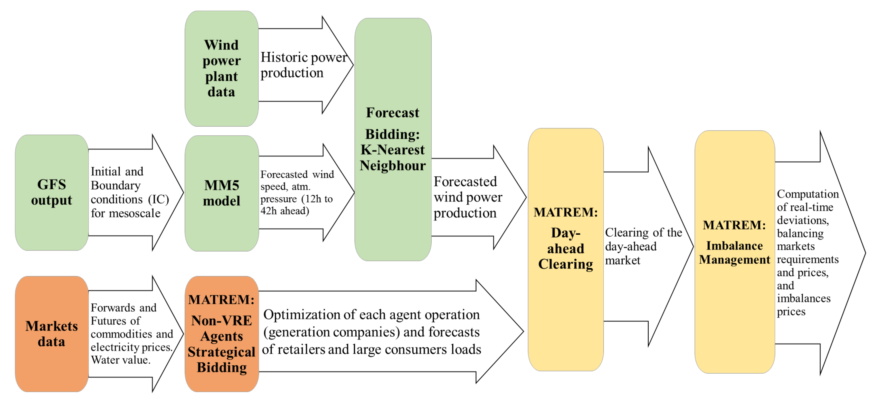
This work makes use of a diverse range of models and involves a set of tasks. Figure 2 depicts a flowchart of the approach considered, highlighting the main tasks and the relationships between them.

4.1. Wind Power Forecast Approach

In the last few years, one of the key scientific research topics is the development of reliable forecasting systems. These systems are being widely employed in different fields, such as the prediction of consumer comfort based on temperature and humidity, electricity demand, wind speed and direction for onshore wind power, and also metocean conditions for offshore wind power, and irradiation for solar power (see, e.g., [43,44,45,46]).

For the particular case of wind power forecast systems, several techniques have been proposed in the literature (see, e.g., [47,48,49,50,51,52]). To support the participation of wind power producers in the DAM, existing wind power forecast systems are generally based on statistical post processing approaches coupled with mesoscale NWP outputs [23]. In this article, a K-nearest neighbour (K-NN) methodology is applied to provide the wind power forecasts. This statistical approach, also known as analogous forecast, has been applied by several authors due to its simplicity, effectiveness and non-parametric features [53,54].

The K-NN methodology is considered a lazy learning methodology, since there is no need to (previously) build a model or a function. Instead, the methodology uses only similar situations from the historical data to forecast. This characteristic is especially suitable to forecast weather dependent variables, such as wind power. The K-NN methodology considers that atmospheric flow releases the same local impact. Consequently, and taking into account the atmospheric flow characteristics, where the meteorological weather patterns have a tendency to repeat over certain regions, from time to time, the wind power forecast production for a determined hour can be determined from a similar meteorological weather pattern from historical events. The K-NN technique has shown a high efficiency in forecasting phenomena where the synoptic variability is predominant, such as precipitation [55] and wind speed [56]. Currently, this technique has already been explored by several authors for forecasting wind power, showing good performance [57,58,59]. To estimate the degree of similarity with each historical event, the Euclidean distance, with a trajectory matrix providing information regarding the state of the atmosphere on the preceding times, is the most common metric used in the wind forecast sector [59].

Due to a large number of degrees of freedom of the atmosphere, it is usual to apply a principal component analysis (PCA) approach to the input data. This procedure allows to filter atmospheric perturbation that represents only background noise [27]. To assist in this filtering process, the North criterion [60] was applied, allowing to identify the appropriate number of principal components (PCs) to be used in each meteorological parameter input.

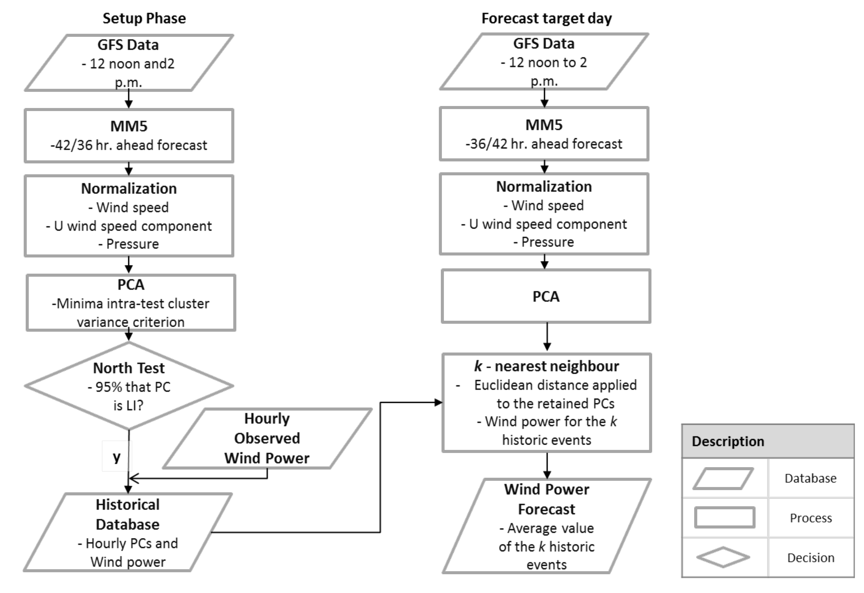
Figure 3 depicts the flowchart of the K-NN methodology applied in this work. In order to calibrate the forecasting methodology, sensitivity studies were performed, using two years of real wind power data from a set of wind parks located in the central region of Portugal. These sensitive tests comprise the suitable number of K nearest neighbours, the size of the trajectory matrix and the selection of the most adequate meteorological parameters. After some tests, the most adequate configuration of the forecast methodology was to set K to 10 using a trajectory matrix with a lag of 3 h, composed by the first three PCs of the longitudinal component of the wind, wind speed, and atmospheric pressure. Thus, the deterministic wind power forecast is based on the average value of the ten historic events.

The normalized root mean square error (NRMSE) represents the quadratic difference between the estimated value (based on the proposed methodologies), and was normalized by the nominal capacity of wind park: $P^{nom}$. The correlation r is used in statistics to measure how strong the relationship is between two variables, in this case, the observed power $P_t^{obs}$ and the forecast power $P_t^{for}$. The F Test is used to verify the statistical significance between the deviations associated with the two different gate-closures considered in this work. Mathematically, the previous parameters are defined by the following equations:

$$NRMSE\left[\%\right]=\sqrt{\frac{\sum {\left(P_t^{obs}-P_t^{for}\right)}^2}{N}}\times \frac{1}{P^{nom}}$$

(1)

$$r=\frac{cov\left(P_t^{obs},P_t^{for}\right)}{\sqrt{var\left(P_t^{obs}\right)var\left(P_t^{for}\right)}}$$

(2)

$$F=\frac{var{\left(P_t^{obs}-P_t^{for1}\right)}^2}{var{\left(P_t^{obs}-P_t^{for2}\right)}^2}$$

(3)

4.2. Selection of Representative Days

The underlying goal of choosing representative days is to statistically detect the most typical wind power daily patterns and, at the same time, clustering together days that exhibit identical patterns. This procedure allows for: (i) feeding the MATREM simulator without resorting to extensively time-consuming simulations, and (ii) assessing, for instance, the typical profiles that can jeopardize the wind power producer revenues enabling for adopting measures to mitigate their risk exposure. The identification of representative days is a suitable approach widely employed to increase the knowledge of a determined parameter allowing the creation of decision support systems (e.g., the classification of the type of profile of electricity customers [61]). A K-medoids clustering algorithm [62] is used in this work to find the representative days based on the daily observed wind power profile for the wind parks considered. This technique allows arranging the input data with similar characteristics into clusters in order to achieve the most representative daily profile. With this step, it is possible to identify (in a statistical way) statistically independent patterns from the data that can be related to physical processes. Clustering algorithms are unsupervised learning processes typically applied to find and split the data according to the similarity among the observations, in a way that is always closer to the elements of the same cluster, and dissimilar among the remaining clusters [62,63].

The main advantages of the K-medoids algorithm, when compared to others non-hierarchical clustering algorithms (e.g., the K-means algorithm) are: (1) to be more robust to noise and outliers by using the median values, and (2) to allow for selecting data points as centres (medoids) [63]. The K-medoids technique used in this work is classified as a non-hierarchical clustering algorithm, allowing to group the data into K clusters. The suitable K, i.e., the number of clusters, is predetermined through the Calinski–Harabasz (CH) criterion [64].

The wind power input matrix ($X_{d,t}$) for the clustering algorithm is defined as follows:

$$X_{d,t}=\left|\begin{array}{cccc}{Z}_{1,1}& Z_{1,2}& \cdots & Z_{1,t}\\ Z_{2,1}& Z_{2,2}& \cdots & Z_{2,t}\\ ⋮& ⋮& ⋮& ⋮\\ Z_{d,1}& Z_{d,2}& \cdots & Z_{d,h}\end{array}\right|$$

(4)

where t represents the wind power observed during a predetermined hour of day d during the period 2009–2010.

4.3. Measures of Economic Results

In this section, the formulation used to compare the results between the 12:00 p.m. scenario (hereafter designated as the base case) and 2:00 p.m. scenario (hereafter designated as the upgraded case) is presented. The total remuneration (per hour) of the wind power producers is as follows:

$$R_t=\sum _{t=0}^{23}{P}_t^{bid}{C}_t^{dayahead}+\left\{\begin{array}{cc}\left(P_t^{obs}-P_t^{bid}\right)C_t^{updeviation},\hfill & \mathrm{f}\mathrm{o}\mathrm{r}{P}_t^{bid}<P_t^{obs}\hfill \\ \left(P_t^{obs}-P_t^{bid}\right)C_t^{downdeviation},\hfill & \mathrm{f}\mathrm{o}\mathrm{r}{P}_t^{bid}>P_t^{obs}\hfill \end{array}\right.$$

(5)

where:

•

${\mathit{C}}_{\mathit{t}}^{\mathit{dayahead}}$ is the day-ahead price at hour t;

•

${\mathit{C}}_{\mathit{t}}^{\mathit{updeviation}}$ and ${\mathit{C}}_{\mathit{t}}^{\mathit{downdeviation}}$ are the up and down deviation costs, respectively.

It is important to note that $P_t^{bid}{C}_t^{dayahead}$ is the part consisting of the remuneration obtained from the day-ahead. The other part consists of the remuneration obtained from the deviations. Therefore, the total remuneration $R_d$ and average remuneration ${\overline{R}}_d$ for a specific day d are as follows:

$$R_d=\sum _{t=0}^{23}{R}_t$$

(6)

$${\overline{R}}_d=\frac{R_d}{{\sum }_{t=0}^{23}{P}_t}$$

(7)

The average remuneration obtained in the day-ahead market ${\overline{R}}_d^{dayahead}$ is defined as follows:

$${\overline{R}}_d^{dayahead}=\frac{{\sum }_{t=0}^{23}{P}_t^{bid}{C}_t^{dayahead}}{{\sum }_{t=0}^{23}{P}_t^{bid}}$$

(8)

In addition, the average remuneration obtained by considering the deviations ${\overline{R}}_d^{deviation}$ is as follows:

$${\overline{R}}_d^{deviation}=\left\{\begin{array}{cc}{\displaystyle \frac{{\sum }_{t=0}^{23}\left(P_t^{obs}-P_t^{bid}\right)C_t^{updeviation}}{{\sum }_{t=0}^{23}\left(P_t^{obs}-P_t^{bid}\right)}},\hfill & \mathrm{f}\mathrm{o}\mathrm{r}{P}_t^{bid}<P_t^{obs}\hfill \\ {\displaystyle \frac{{\sum }_{t=0}^{23}\left(P_t^{obs}-P_t^{bid}\right)C_t^{downdeviation}}{{\sum }_{t=0}^{23}\left(P_t^{obs}-P_t^{bid}\right)}},\hfill & \mathrm{f}\mathrm{o}\mathrm{r}{P}_t^{bid}>P_t^{obs}\hfill \end{array}\right.$$

(9)

With these formulae, it is possible to compute the average wind power value, the energy transacted in the tertiary reserve market, and the tertiary reserve cost for both scenarios. Both the reserve cost and the electric system levelized cost are computed by taking into account the occurrence of each representative day and the traded energy. In order to assess the gain effect regarding the proposed adaptation of the gate closure of the day-ahead market, several key performance indicators (KPIs) are defined (see

Table 1. KPIs considered in this work.

KPI	Objective	Formulation
Increase in the wind power value to the market	Increase the remuneration of wind power producers in the market	Equation (7)
Increase in the forecast accuracy	Reduce the forecast error	Equation (3)
Reduction of total control reserve by wind power forecast improvements	Reduce the balanceneeds of thetertiary reserve	Equations (1) and (2)
Reduction of the tertiary reserve costs	Reduce the balance costs of the tertiary reserve	Tertiary reserve simulation
Reduction of total operating costs in the electricity system by forecast improvements	Reduce the system costs with the day-ahead market and the tertiary reserve	Day-ahead market and tertiary reserve simulations

).

5. The Case Study

This section describes a case study to analyse the effect of wind power forecasts errors on the outcomes of the DAM. The following two scenarios are considered: (i) a base scenario, where the DAM closes at 12:00 p.m. (the bids of the wind power producers are based on a wind forecast performed 18 to 42 h ahead), and (ii) an updated scenario, where the DAM closes at 2:00 p.m. (the bids of WPPs are based on an updated forecast performed 12 to 36 h ahead).

5.1. Software Agents and Wind Power Profiles

This study makes use of data published by the Iberian electricity market (MIBEL) and involves the simulation of the day-ahead market prices as well as the balancing market prices. Market participants are modeled as software agents, defined with the help of the MATREM system. Since the normal operation of the daily market of MIBEL involves a number of bids on the order of thousands for a particular hour, there is a need to make some simplifications related to the number of software agents, in order to avoid a large computational complexity. Accordingly, the main agents considered in the study are as follows: a market operator (S1), a system operator (S2), twelve producers (supply-side agents) and four retailers (demand-side agents).

Table 2. Producer agents (software agents) and their key characteristics.

Agent	Country	Technology	Maximum Capacity (MW)	Marginal Cost (€/MWh)
P1	Portugal	Wind	2500	0
P2	Portugal	Renewable mix	2000	0
P3	Portugal	Hydroelectricity	4500	$\left[30;60\right]$
P4	Portugal	Coal	1800	≈30
P5	Portugal	Combined Cycle Gas	3000	≈55
P6	Portugal	Fuel oil	2000	≈70
P7	Spain	Renewable mix	30,000	0
P8	Spain	Hydroelectricity	16,500	$\left[30;60\right]$
P9	Spain	Coal	10,000	≈30
P10	Spain	Nuclear	7500	≈30
P11	Spain	Combined Cycle Gas	22,000	≈55
P12	Spain	Fuel oil	4000	≈70

presents the characteristics of the supply-side agents. The wind aggregator (agent $P_1)$ represents the Portuguese wind farms.

It is important to note that the detection of violations related to the interconnection constraints between Portugal and Spain leads to a process of market splitting, resulting in different price areas for Portugal and Spain. After a careful examination, we concluded that this situation applies for some hours of the days under consideration. In practice, this means two sets of simulation for each hour of operation, one for Portugal and another for Spain. However, for convenience, and in the interests of simplicity, the day-ahead market is cleared for Portugal only.

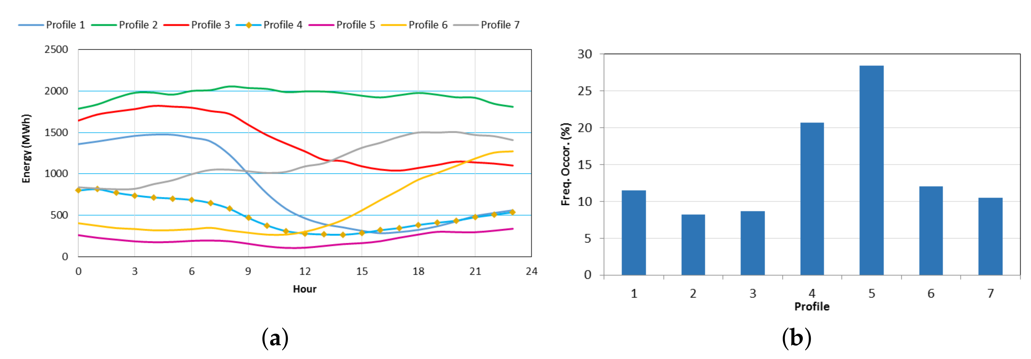
The forecast methodology is deterministic and uses the following: (i) numerical weather prediction data outputs (see Section 4), and (ii) observed data for a set of wind farms during the period 2009–2010. The wind farms have a nominal capacity of 250 MW (10% of the Portuguese installed capacity, in 2010). This value is upscaled to 2500 MW to obtain a meaningful impact on the market results. The observed wind power profiles are depicted in Figure 4a. The representability of each wind power profile is also shown in Figure 4b.

The analysis of Figure 4 supports the consideration that the Portuguese wind farms are located in a mountain region, since several wind power profiles show the typical features of wind speed in such a region (although with different intensity)—that is, due to the thermal stratification and local effects [65], the highest wind speed is associated with the nocturnal period. Moreover, the most common wind power profile shows a reduced production during all day. On the other hand, profile 2 is associated with a high level of wind power production, which occurs during the passage of severe meteorological phenomena, as the cyclone systems [66]. This profile shows the lowest number of occurrences.

5.2. Wind Power Forecast Deviations

Figure 5 depicts the wind power forecast deviations (forecast minus observed production) for the seven representative days, at 12:00 p.m. (base case, left) and 2:00 p.m. (updated case, right). The figure shows that the wind power forecast deviations at 12:00 p.m. have an absolute value that is almost twice that of the deviations at 2:00 p.m. Moreover, wind power fluctuations are considerably higher in the base scenario. For instance, the uncertainty in profile 2 ranges between −200 and 1700 MW.

Table 3. Correlation and NRMSE between the observed and forecasted wind power and F value of the wind power deviations for each scenario and wind power profile.

Parameter Difference	Simulation	Wind Power Profile
		1	2	3	4	5	6	7
Correlation	Base Scenario	0.91	−0.35	0.72	0.54	0.79	0.78	0.47
	Upgrade Scenario	0.95	0.27	0.89	0.86	0.92	0.88	0.71
NRMSE (%)	Base Scenario	4.23	19.46	10.72	12.45	2.73	5.99	8.94
	Upgrade Scenario	2.87	12.85	3.93	5.52	2.10	3.90	5.61
F	Both Scenario	2.07	3.39	2.61	2.81	2.37	1.94	3.85

depicts the forecast results regarding both the NRMSE and the correlation values between the two scenarios. The most significant improvement was observed in profile 2. This profile, usually associated to extreme weather conditions, shows a strong improvement in the correlation and the NRMSE values. The link between wind power variability as well as the uncertainty with extreme weather conditions was described by several authors [23,66,67,68,69], who demonstrated that larger errors in the wind power forecast are expected to occur during severe weather conditions with strong dynamics (e.g., storms and cold fronts) when compared with weather conditions associated with stationary systems (e.g., anticyclonic systems). For a 0.05 significance level, the critical value is 2.01, which means that comparing both deviations (see Figure 5), exist statistically differences in all profiles, except in profile 6 (see Table 3).

Profile 4 also shows a strong improvement in the wind power forecast for the upgrade scenario. Profile 5 shows the lowest NRMSE amelioration that can be explained with the capabilities to obtain a reliable forecast during calm wind speed conditions [67,69]. Consequently, results from Table 3 highlighted the fact that the data considered about the ICs strictly define the wind power forecast errors. Thus, as expected, since the most up-to-date information on the state of the atmosphere is used, postponing the gate closure can strongly reduce the uncertainty of the bids that the wind power producers submit to the day-ahead market.

5.3. Simulation Results

5.3.1. Impact of Wind Power Forecast on Market Outcomes

In a preliminary attempt to understand the relation of the aforementioned wind power forecast uncertainty results with the market outcomes, we observed that the deviations are essentially positive in most of the representative days (day seven is the exception), meaning that the forecasts normally underestimate the wind power values. From the point-of-view of wind power producers, this situation (underestimation) can be profitable, since wind power is offered at a price around 0 in the day-ahead market, and thus an underestimation forecast will increase the market price. On the other hand, an overestimation forecast can decrease the day-ahead market price, decreasing the wind energy value. Therefore, it can be concluded that an underestimation of the wind power production in the day-ahead market (shortage forecast) overestimates the importance of the wind power and also gives an extra amount to the supply-side agents (by increasing the market-clearing price). On the other hand, an overestimation of the wind power production (excess forecast) undervalues the wind power value. Moreover, due to the payment of penalties in the balancing market, the latter situation can lead to a drastic reduction in the revenues of wind power producers. Thus, an underestimation of wind power production can be more profitable for wind power producers.

The results of the simulations for both the base scenario (12:00 p.m.) and the updated scenario (2:00 p.m.) are presented in

Table 4. Key results for the base scenario (12:00 p.m. scenario).

Profile	Power Forecast 12 h (Base Scenario)
	1	2	3	4	5	6	7
Day-ahead energy bid (GWh)	22.01	25.93	22.18	14.37	10.58	8.06	12.61
Day-ahead Remuneration (k€)	767.21	951.6	885.58	529.22	389.25	317.03	525.92
Average Day-ahead Rem. (€/MWH)	34.85	36.7	39.93	36.82	36.81	39.31	41.72
Real time deviations (MWh)	4.45	21.86	11.61	13.26	2.55	5.5	8.78
Deviations Revenue (k€)	−143.6	460.33	226.29	317.29	9.94	98.66	−527.7
Average Remuneration (€/MWh)	29.94	30.03	32.91	30.63	33.75	31.75	−0.46
Total Remuneration (k€)	623.62	1411.9	111.19	846.51	399.19	415.69	−1.77

and

Table 5. Key results for the updated scenario (2:00 p.m. scenario).

Profile	Power Forecast 2:00 p.m. (Updated Scenario)
	1	2	3	4	5	6	7
Day-ahead energy bid (GWh)	20.62	32.48	30.83	22.59	13.41	10.26	9.83
Day-ahead Remuneration (k€)	699.61	1173.3	1187.7	784.42	488.76	400.31	414.5
Average Day-ahead Rem. (€/MWh)	33.93	36.12	38.53	34.73	36.44	39.03	42.17
Real-time deviations (MWh)	2.76	14.59	3.78	5.2	1.75	3.82	6.01
Deviations Revenue (k€)	−45.3	330.82	48.19	124.78	−81.56	43.28	−355.6
Average Remuneration (€/MWh)	31.42	31.99	36.58	32.9	34.43	33.88	15.41
Total Remuneration (€k)	654.31	1504.1	123.59	909.2	407.2	443.6	58.94

, respectively. In both tables, details regarding the outcomes of postponing the market closing time by two hours are also provided. As mentioned previously, the sum of the wind power deviations at 12:00 p.m. is almost twice the deviations associated with 2:00 p.m., and on some days it is more than twice the amount, such as the 3rd and 4th representative days. The results also show that the underestimation of wind power production can increase the market price and, as discussed previously, can overvalue the wind power. This conclusion takes into account the fact that the average day-ahead remuneration is higher at 12:00 p.m., in almost all days, excluding the 7th representative day. In this representative day, the overestimation of wind power production leads to an undervaluation of the wind power value. This behavior can also be observed in the revenue deviations results. In fact, when both day-ahead and revenue deviations are positive, an underestimation of wind power is obtained. Consequently, power producers receive a positive revenue for the extra energy at the real-time operation (normally less than in the day-ahead market, due to penalties). When the revenue deviations are negative, this normally means an overestimation of wind power production when compared with the forecast, so there will be a need to pay a value higher than the day-ahead price.

One of the key parameters that can be used to compare the base scenario with the updated scenario is the average remuneration of the wind power producers. Considering both tables, it can be seen that, in the updated scenario, the wind value (average remuneration of the wind power) is always higher, and the proposed market design element seems even more relevant when a wind power forecast overestimation occurs. For instance, for the 7th representative day, the average remuneration of the wind power producer is negative, in the base case. Therefore, if hypothetically wind power producers are active players in the market, with the current market design, when the day-ahead market prices are lower than the deviation prices, the producers who have an energy shortage (when compared to their energy forecast bids) may have a negative average remuneration.

Now, taking into account the representability of each wind power profile during the two years of data, it is possible to compute the average wind energy value, the energy transacted in the tertiary reserve market, and the tertiary reserve costs, among other key parameters, for both the 12:00 p.m. and the 2:00 p.m. scenarios (see

Table 6. Average values of the key parameters under evaluation per day.

Key Parameters	Simulations
	12:00 p.m.	2:00 p.m.
	(Base Scenario)	(Updated Scenario)
Wind Energy Value (€/MWh)	28.46	31.69
Forecast NRMSE (%)	8.03	4.52
Reserve Use (GWh)	11.1	6.23
Reserve Direction (GWh)	−7.44	−3.83
Reserve Costs (M€)	−0.1	−0.04
Reserve Levelized Cost (€/MWh)	−7.26	−3.83
Down Reserve Price (€/MWh)	20.07	25.7
Day-ahead Market Cost (M€)	18.75	18.63
Day-ahead Market Prices (€/MWh)	38.6	37.97
Day-ahead Market Energy (GWh)	487.71	491.31
Electric System Cost (M€)	18.65	18.58
Electric System Lev. Cost (€/MWh)	38.84	38.12

). The results in the Table show that the upgraded case leads to better results in almost all key indicators (the exception is the reserve cost).

Also, the results suggest that a reduction in the day-ahead market prices, due to a reduction in the forecast errors (NRMSE), leads to an increase in the wind power producers revenues, by allowing for reducing their losses associated with the deviation penalties. With a reduction of forecast errors, the quantity of reserve required to compensate the deviations decreases. However, both the reserve levelized cost and the reserve cost increased. These results are associated with a decrease in the system requirements for down reserve (see the reserve direction parameter). In this way, the system operator receives an inferior remuneration from the down reserve, which leads to an increase of the down reserve price. This increase, together with a decrease in the down reserve utilization and the day-ahead market prices, will negatively affect the revenue of the power plants that bid at the tertiary reserve market. This behavior is associated with a reduction of the remuneration of wind power producers from the day-ahead market since they need to pay a high price for the down reserve, for a small quantity of energy.

5.3.2. Quantifying the Gain Effect of the Proposed Market Design Change

The KPIs defined in Section 4 enable for quantifying the gain effect by setting the gate closure of the day-ahead market to 2:00 p.m., instead of 12:00 p.m. (see

Table 7. Key performance indicators (KPIs).

KPIs (%)	Changing from 12:00 p.m. to 2:00 p.m.
Increase in the wind power value to the market	11.34
Increase in the forecast accuracy	43.71
Reduction of total control reserve by forecast improvements in wind power	43.87
Reduction of the tertiary reserve costs	−56.25
Reduction of total operating costs in the electricity system by forecast improvements	16.46

). The change of the day-ahead market closing time brings benefits to the system in general, with a reduction around 16.5% in the total costs. As stated before, the wind power producers and the demand-side players benefit from this change. Wind power producers gain from selling the same quantity at a higher net price (market price with fewer penalties). The demand-side players gain from buying a similar quantity of electricity at a lower price. The system operator benefits from using less the reserve market to balance the system (a reduction around 44%) and also receives the lowest revenue (less 56%) from the down reserve market (part of the tertiary reserve market), which means that the agents that deviate will pay higher penalties. Notwithstanding, the power producers that buy energy from the tertiary reserve market (down reserve) decrease their revenues, by having less energy to buy at a higher price.

A comparison of the results shown in Table 7 with the main results presented by the literature (see Section 2) allows us to conclude that postponing the gate-closure of the day-ahead market only two hours seems to be a change of market design that can bring large benefits to power systems generally.

6. Conclusions

The article analyzed a change in the gate closure of the day-ahead market to deal with the uncertainty of variable generation. Specifically, it considered the adjustment of the day-ahead market closing time from 12:00 p.m. (currently in use in most of the European electricity markets) to 2:00 p.m. (CET). To test this adjustment, a case study based on real data from a set of aggregated wind parks in Portugal, and also data from the supply-side (producers) and demand-side (retailers buying electricity for the end-use consumers) of the Iberian Market (MIBEL), as an approximation of the entire system, was established.

Wind power forecast data were obtained using a K-NN approach based on data from a NWP model. The day-ahead market was simulated using the system marginal pricing algorithm for seven representative days, taking into account two scenarios: gate closure of the day-ahead market set to 12:00 p.m. (base case) and to 2:00 p.m. (updated case). The seven representative wind power production days enable: (i) to simulate only the most common typical wind power production days in the region under study, and (ii) to identify the wind power profiles that can jeopardise the revenues of the wind power producers or can pose serious challenges to transmission system operators.

From a wind power forecast perspective, the results show that some wind power profiles clearly benefit from a change in the market design. Regarding the electricity market perspective, the results show that the change of the day-ahead market closing time to 2:00 p.m. benefits the wind power producers at both a technical and financial level by decreasing the forecast errors and increasing the revenues. The consumers can also potentially take advantage of this change due to a potential reduction in the overall system costs, which may allow a reduction of the electricity tariffs. The system operator benefits from a reduction in the wind park forecast errors, by reducing the requirements to maintain the production/demand balance (technical benefit), requiring less energy from the tertiary reserve market. However, they also receive less money from the downregulation (financial loss), which means that the agents that deviate will need to pay higher penalties to compensate this loss. The power producers that bid at the down reserve market have a loss due to a decrease in the system requirements for this type of reserve, i.e., the system operator requires less down reserve quantity to balance the system, which increases the price of this market.

The results presented in this work highlight that electricity markets with high shares of VRE could benefit from DAMs with a gate closure closer to real-time operation, due to improvements in the forecast accuracy. The full integration of wind power in markets can be possible with substantial changes to the current market designs, especially in power systems with a high share of VRE integration, as expected in the forthcoming years with the society decarbonization.

References

- Conejo, A.J.; Carrión, M.; Morales, J.M. Decision Making under Uncertainty in Electricity Markets; Springer: New York, NY, USA, 2010. [Google Scholar]
- Lopes, F.; Coelho, H. Electricity Markets with Increasing Levels of Renewable Generation: Structure, Operation, Agent-Based Simulation and Emerging Designs; Springer International Publishing: Cham, Switzerland, 2018. [Google Scholar]
- Ela, E.; Milligan, M.; Bloom, A.; Cochran, J.; Botterud, A.; Townsend, A.; Levin, T. Overview of Wholesale Electricity Markets. In Electricity Markets with Increasing Levels of Renewable Generation: Structure, Operation, Agent-Based Simulation and Emerging Designs; Springer International Publishing: Cham, Switzerland, 2018; pp. 3–21. [Google Scholar]
- Moiseeva, E.; Wogrin, S.; Hesamzadeh, M.R. Generation flexibility in ramp rates: Strategic behavior and lessons for electricity market design. Eur. J. Oper. Res. 2017, 261, 755–771. [Google Scholar] [CrossRef]
- Ela, E.; Milligan, M.; Bloom, A.; Botterud, A.; Townsend, A.; Levin, T. Incentivizing Flexibility in System Operations. In Electricity Markets with Increasing Levels of Renewable Generation: Structure, Operation, Agent-Based Simulation, and Emerging Designs; Springer International Publishing: Cham, Switzerland, 2018; pp. 95–127. [Google Scholar]
- Algarvio, H.; Lopes, F.; Couto, A.; Estanqueiro, A. Participation of Wind Power Producers in Day-ahead and Balancing Markets: An Overview and a Simulation-based Study. WIREs Energy Environ. 2019, 2019, e343. [Google Scholar] [CrossRef]
- Vilim, M.; Botterud, A. Wind power bidding in electricity markets with high wind penetration. Appl. Energy 2014, 118, 141–155. [Google Scholar] [CrossRef]
- IRENA. Adapting Market Design to High Shares of Variable Renewable Energy; International Renewable Energy Agency: Abu Dhabi, UAE, 2017. [Google Scholar]
- Roques, F.; Finon, D. Adapting electricity markets to decarbonisation and security of supply objectives: Toward a hybrid regime? Energy Policy 2017, 105, 584–596. [Google Scholar] [CrossRef]
- Zhang, C.; Yan, W. Spot Market Mechanism Design for the Electricity Market in China Considering the Impact of a Contract Market. Energies 2019, 12, 1064. [Google Scholar] [CrossRef]
- International Energy Agency. The Power of Transformation: Wind, Sun and the Economics of Flexible Power Systems; International Energy Agency: Paris, France, 2014. [Google Scholar]
- European Commission. Proposal for a Regulation of the European Parliament and of the Council on the Internal Market for Electricity. February 2017. Available online: http://ec.europa.eu/energy/sites/ener/files/documents/1underlinetag|enunderlinetag|actunderlinetag|part1underlinetag|v9.pdf (accessed on 5 July 2019).
- Algarvio, H.; Lopes, F.; Couto, A.; Santana, J.; Estanqueiro, A. Effects of Regulating the European Internal Market on the integration of Variable Renewable Energy. WIREs Energy Environ. 2019, 2019, e346. [Google Scholar] [CrossRef]
- Algarvio, H.; Couto, A.; Lopes, F.; Estanqueiro, A.; Santana, J. Multi-Agent Energy Markets with High Levels of Renewable Generation: A Case-Study on Forecast Uncertainty and Market Closing Time. In Proceedings of the 13th International Conference Distributed Computing and Artificial Intelligence, Sevilla, Spain, 1–3 June 2016; pp. 339–347. [Google Scholar]
- Algarvio, H.; Couto, A.; Lopes, F.; Estanqueiro, A.; Holttinen, H.; Santana, J. Agent-Based Simulation of Day-Ahead Energy Markets: Impact of Forecast Uncertainty and Market Closing Time on Energy Prices. In Proceedings of the 27th Workshop on Database and Expert Systems Applications (DEXA 2016), Porto, Portugal, 5–8 September 2016; pp. 166–170. [Google Scholar]
- Algarvio, H.; Couto, A.; Lopes, F.; Estanqueiro, A.; Santana, J. Multi-agent Wholesale Electricity Markets with High Penetrations of Variable Generation: A Case-study on Multivariate Forecast Bidding Strategies. In Highlights of Practical Applications of Cyber-Physical Multi-Agent Systems; Springer: Cham, Switzerland, 2017; pp. 340–349. [Google Scholar]
- Burgholzer, B.; Fontaine, A.; Galmiche, F.; Völler, S.; Jaehnert, S.; Chicharro, F.; Camacho, L.; Ahcin, P. D5.2 Report on the quantitative evaluation of policies for post 2020 RES-E targets. Market4RES Report. September 2016. Available online: http://market4res.eu/wp-content/uploads/D5-2_final-003.pdf (accessed on 17 July 2019).
- Wooldridge, M. An Introduction to Multiagent Systems; Wiley: Chichester, UK, 2009. [Google Scholar]
- Lopes, F. MATREM: An Agent-based Simulation Tool for Electricity Markets. In Electricity Markets with Increasing Levels of Renewable Generation: Structure, Operation, Agent-Based Simulation and Emerging Designs; Springer: Cham, Switzerland, 2018; pp. 189–225. [Google Scholar]
- Lopes, F.; Coelho, H. Electricity Markets and Intelligent Agents. Part II: Agent Architectures and Capabilities. In Electricity Markets with Increasing Levels of Renewable Generation: Structure, Operation, Agent-Based Simulation and Emerging Designs; Springer: Cham, Switzerland, 2018; pp. 49–77. [Google Scholar] [CrossRef]
- Kahn, P. Numerical Techniques for Analysing Market Power in Electricity. Electr. J. 1998, 11, 34–43. [Google Scholar] [CrossRef]
- Hobbs, F. Linear Complementarity Models of Nash-Cournot Competition in Bilateral and POOLCO Power Markets. IEEE Trans. Power Syst. 2001, 16, 194–202. [Google Scholar] [CrossRef]
- Giebel, G.; Brownsword, R.; Kariniotakis, G.; Denhard, M.; Draxl, C. The State-of-the-Art in Short-Term Prediction of Wind Power: A Literature Overview. Deliverable Report D-1.2, Project ANEMOS.Plus, Contract 038692, DTU. 2011, p. 106. Available online: https://orbit.dtu.dk/fedora/objects/orbit:83397/datastreams/file_5277161/content (accessed on 17 July 2019).
- Jung, J.; Broadwater, R. Current Status and Future Advances for Wind Speed and Power Forecasting. Renew. Sustain. Energy Rev. 2014, 31, 762–777. [Google Scholar] [CrossRef]
- Grell, G.; Dudhia, J.; Stauffer, D.R. A Description of the Fifth-Generation Penn State/NCAR Mesoscale Model (MM5). NCAR Technical Note NCAR/TN-398+STR. 1995, p. 121. Available online: http://opensky.ucar.edu/islandora/object/technotes%3A170/datastream/PDF/view (accessed on 17 July 2019).
- Lorenz, E.N. Deterministic Nonperiodic Flow. J. Atmos. Sci. 1963, 20, 130–141. [Google Scholar] [CrossRef] [Green Version]
- Couto, A.; Rodrigues, L.C.; Costa, P.; Silva, J.; Estanqueiro, A. Wind power participation in electricity markets—The role of wind power forecasts. In Proceedings of the 16th IEEE International Conference on Environment and Electrical Engineering, Florence, Italy, 7–10 June 2016; p. 6. [Google Scholar]
- Alvarez, I.; Gomez-Gesteira, M.; Carvalho, D. Deep-Sea Research II Comparison of different wind products and buoy wind data with seasonality and interannual climate variability in the southern Bay of Biscay (2000–2009). Deep Sea Res. Part II 2014, 106, 38–48. [Google Scholar] [CrossRef]
- Wang, A.; Zeng, X. Evaluation of multireanalysis products with in situ observations over the Tibetan Plateau. JGR Atmos. 2012, 117, 1–12. [Google Scholar] [CrossRef]
- Soukissian, T.H.; Papadopoulos, A. Effects of different wind data sources in offshore wind power assessment. Renew. Energy 2015, 77, 101–114. [Google Scholar] [CrossRef]
- Rutledge, G.K.; Alpert, J.; Ebisuzaki, W. NOMADS: A Climate and Weather Model Archive at the National Oceanic and Atmospheric Administration. Bull. Am. Meteorol. Soc. 2006, 87, 327–341. [Google Scholar] [CrossRef]
- ACER. Annual Report on the Results of Monitoring the Internal Electricity and Gas Markets in 2016. Electricity Wholesale Markets Volume. October 2017. Available online: http://www.acer.europa.eu/Official_documents/Acts_of_the_Agency/Publication/ACER%20Market%20Monitoring%20Report%202016%20-%20ELECTRICITY.pdf (accessed on 5 July 2019).
- Skytte, K.; Bobo, L. Increasing the value of wind: From passive to active actors in multiple power markets. WIREs Energy Environ. 2019, 8. [Google Scholar] [CrossRef]
- Mills, A.; Wiser, R. Changes in the economic value of wind energy and flexible resources at increasing penetration levels in the Rocky Mountain Power Area. Wind Energy 2014, 17, 1711–1726. [Google Scholar] [CrossRef]
- Holttinen, H.; Miettinen, J.; Couto, A.; Algarvio, H.; Rodrigues, L. Wind power producers in shorter gate closure markets and balancing markets. In Proceedings of the 13th International Conference on the European Energy Market, Porto, Portugal, 6–9 June 2016; p. 5. [Google Scholar]
- Holttinen, H.; Milligan, M.; Ela, M.; Menemenlis, N.; Dobschinski, J.; Rawn, B.; Bessa, R.J.; Flynn, D.; Gomez Lazaro, E.; Detlefsen, N. Methodologies to determine operating reserves due to increased wind power. IEEE Trans. Sustain. Energy 2012, 3, 713–723. [Google Scholar] [CrossRef]
- Milligan, M.; Kirby, B.; Holttinen, H.; Kiviluoma, J.; Estanqueiro, A.; Martín-Martínez, S.; van Hulle, F.; Gomez-Lázaro, E.; Pineda, I.; Smith, J.C. Wind Integration Cost and Cost-Causation; National Renewable Energy Lab. (NREL): Golden, CO, USA, 2013; p. 6. [Google Scholar]
- González-Aparicio, I.; Zucker, A. Impact of wind power uncertainty forecasting on the market integration of wind energy in Spain. Appl. Energy 2015, 159, 334–349. [Google Scholar] [CrossRef]
- Algarvio, H.; Lopes, F.; Santana, J. Bilateral Contracting in Multi-agent Energy Markets: Forward Contracts and Risk Management. In Highlights of Practical Applications of Agents, Multi-Agent Systems, and Sustainability: The PAAMS Collection (PAAMS 2015); Springer International Publishing: Cham, Switzerland, 2015; pp. 260–269. [Google Scholar]
- Sousa, F.; Lopes, F.; Santana, J. Contracts for Difference and Risk Management in Multi-agent Energy Markets. In Advances in Practical Applications of Agents, Multi-Agent Systems, and Sustainability: The PAAMS Collection (PAAMS 2015); Springer International Publishing: Cham, Switzerland, 2015; pp. 339–347. [Google Scholar]
- Lopes, F.; Mamede, N.; Novais, A.Q.; Coelho, H. A Negotiation Model for Autonomous Computational Agents: Formal Description and Empirical Evaluation. J. Intell. Fuzzy Syst. 2002, 12, 195–212. [Google Scholar]
- Lopes, F.; Coelho, H. Concession Behaviour in Automated Negotiation. In E-Commerce and Web Technologies; Springer: Berlin/Heidelberg, Germany, 2010; pp. 184–194. [Google Scholar] [Green Version]
- Dong, Y.; Zhang, Z.; Hong, W.C. A hybrid seasonal mechanism with a chaotic cuckoo search algorithm with a support vector regression model for electric load forecasting. Energies 2018, 11, 1009. [Google Scholar] [CrossRef]
- Capizzi, G.; Lo Sciuto, G.; Napoli, C.; Tramontana, E. Advanced and adaptive dispatch for smart grids by means of predictive models. IEEE Trans. Smart Grid 2017, 9, 6684–6691. [Google Scholar] [CrossRef]
- Brusca, S.; Capizzi, G.; Lo Sciuto, G.; Susi, G. A new design methodology to predict wind farm energy production by means of a spiking neural network-based system. Int. J. Numer. Model. 2019, 32, e2267. [Google Scholar] [CrossRef]
- Hong, W.C.; Li, M.W.; Geng, J.; Zhang, Y. Novel chaotic bat algorithm for forecasting complex motion of floating platforms. Appl. Math. Model. 2019, 72, 425–443. [Google Scholar] [CrossRef]
- Lenzi, A.; Steinsland, I.; Pinson, P. Benefits of spatiotemporal modeling for short-term wind power forecasting at both individual and aggregated levels. Environmentrics 2018, 29, e2493. [Google Scholar] [CrossRef]
- Ohba, M.; Kadokura, S.; Nohara, D. Medium-Range Probabilistic Forecasts of Wind Power Generation and Ramps in Japan Based on a Hybrid Ensemble. Atmosphere 2018, 9, 423. [Google Scholar] [CrossRef]
- Agarwal, P.; Shukla, P.; Sahay, K.B. A Review on Different Methods of Wind Power Forecasting. In Proceedings of the 2018 International Electrical Engineering Congress (iEECON), Krabi, Thailand, 7–9 March 2018; pp. 1–4. [Google Scholar]
- Liu, H.; Chen, C.; Lv, X.; Wu, X.; Liu, M. Deterministic wind energy forecasting: A review of intelligent predictors and auxiliary methods. Energy Convers. Manag. 2019, 195, 328–345. [Google Scholar] [CrossRef]
- Zhang, J.; Cui, M.; Hodge, B.M.; Florita, A.; Freedman, J. Ramp forecasting performance from improved short-term wind power forecasting over multiple spatial and temporal scales. Energy 2017, 122, 528–541. [Google Scholar] [CrossRef] [Green Version]
- Ellis, N.; Davy, R.; Troccoli, A. Predicting wind power variability events using different statistical methods driven by regional atmospheric model output. Wind Energy 2015, 18, 1611–1628. [Google Scholar] [CrossRef]
- Martínez, F.; Pérez, M.D.; Frías, M.P.; Rivera, A.J. A methodology for applying k -nearest neighbor to time series forecasting. Artif. Intell. Rev. 2017. [Google Scholar] [CrossRef]
- Taneja, S.; Gupta, C.; Goyal, K.; Gureja, D. An Enhanced K-Nearest Neighbor Algorithm Using Information Gain and Clustering. In Proceedings of the 2014 Fourth International Conference on Advanced Computing & Communication Technologies, Rohtak, India, 8–9 February 2014; pp. 325–329. [Google Scholar]
- Zorita, E.; Von Storch, H. The Analog Method as a Simple Statistical Downscaling Technique: Comparison with More Complicated Methods. J. Clim. 1999, 12, 2474–2489. [Google Scholar] [CrossRef]
- Pascual, A.; Valero, F.; Martín, M.L.; Morata, A.; Luna, M.Y. Probabilistic and deterministic results of the ANPAF analog model for Spanish wind field estimations. Atmos. Res. 2012, 108, 39–56. [Google Scholar] [CrossRef]
- Alessandrini, S.; Sperati, S.; Pinson, P. A comparison between the ECMWF and COSMO Ensemble Prediction Systems applied to short-term wind power forecasting on real data. Appl. Energy 2013, 107, 271–280. [Google Scholar] [CrossRef]
- Martín, M.L.; Valero, F.; Pascual, A.; Sanz, J.; Frias, L. Analysis of wind power productions by means of an analog model. Atmos. Res. 2014, 143, 238–249. [Google Scholar] [CrossRef]
- Junk, C.; Delle Monache, L.; Alessandrini, S.; Cervone, G.; von Bremen, L. Predictor-weighting strategies for probabilistic wind power forecasting with an analog ensemble. Meteorol. Zeitschrift 2015, 24, 361–379. [Google Scholar] [CrossRef]
- North, G.; Bell, T. Sampling errors in the estimation of empirical orthogonal functions. Mon. Weather Rev. 1982, 110, 699–706. [Google Scholar] [CrossRef]
- Ramos, S.; Duarte, J.; Soares, J.; Vale, Z.; Duarte, F. Typical Load Profiles in the Smart Grid Context—A Clustering Methods Comparison. In Proceedings of the IEEE Power and Energy Society General Meeting 2012, San Diego, CA, USA, 22–26 July 2012. [Google Scholar]
- Park, H.S.; Jun, C.H. A simple and fast algorithm for K-medoids clustering. Expert Syst. Appl. 2009, 36, 3336–3341. [Google Scholar] [CrossRef]
- Huth, R.; Beck, C.; Philipp, A.; Demuzere, M.; Ustrnul, Z.; Cahynová, M.; Kyselý, J.; Tveito, O.E. Classifications of atmospheric circulation patterns: Recent advances and applications. Ann. N. Y. Acad. Sci. 2008, 1146, 105–152. [Google Scholar] [CrossRef]
- Calinski, T.; Harabasz, J. A dendrite method for cluster analysis. Commun. Stat. 1974, 3, 27. [Google Scholar]
- Draxl, C. On the Predictability of Hub Height Winds. Ph.D. Thesis, DTU Wind Energy, Roskilde, Denmark, 2012; p. 105. [Google Scholar]
- Couto, A.; Costa, P.; Rodrigues, L.; Lopes, V.; Estanqueiro, A. Impact of Weather Regimes on the Wind Power Ramp Forecast in Portugal. IEEE Trans. Sustain. Energy 2015, 6, 934–942. [Google Scholar] [CrossRef]
- Lange, M.; Heinemann, D. Relating the uncertainty of short-term wind speed predictions to meteorological situations with methods from synoptic climatology. In Proceedings of the European Wind Energy Conference EWEC, Madrid, Spain, 16–19 June 2003; p. 7. [Google Scholar]
- Ernst, B.; Oakleaf, B.; Ahlstrom, M.L.; Lange, M.; Moehrlen, C.; Lange, B.; Focken, U.; Rohrig, K. Predicting the wind. IEEE Power Energy Mag. 2007, 5, 78–89. [Google Scholar] [CrossRef]
- Trancoso, R. Operational Modelling as a Tool in Wind Power Forecast and Meteorological Warnings. Ph.D. Thesis, Instituto Superior Técnico, Lisbon, Portugal, 2012; p. 146. [Google Scholar]
Figure 1.
Global Forecast System (GFS) data availability and DAM design: (top)—actual; (bottom)— proposed in this work.
Figure 2.
Overview of the methodology considered in this work, specifically the method and the main tasks related to the definition of the bids of the wind power producer (green) and the other market participants (light orange), as well as the procedure associated with the operation of the day-ahead market and the imbalance management process (light yellow).
Figure 3.
Wind power forecasts methodology based on NWP data coupled with a K-NN approach.
Figure 4.
Wind energy typical profile (a) and representability of each wind power profile during the 2-year period of the study (b).
Figure 5.
Wind power forecast deviations at 12:00 p.m. (base case, left) and at 2:00 p.m. (updated case, right).