Identification of Low Frequency Oscillations Based on Multidimensional Features and ReliefF-mRMR

1
School of Electrical Engineering, Southeast University, Nanjing 210096, China
2
Jiangsu Provincial Key Laboratory of Smart Grid Technology and Equipment, Southeast University, Nanjing 210096, China
*
Author to whom correspondence should be addressed.
Energies 2019, 12(14), 2762; https://doi.org/10.3390/en12142762
Submission received: 26 June 2019
/
Revised: 9 July 2019
/
Accepted: 17 July 2019
/
Published: 18 July 2019
(This article belongs to the Special Issue Application of Machine Learning and Data Mining in Electrical Engineering)
Abstract
:Low frequency oscillations (LFOs) in power systems usually fall into two types, i.e., forced oscillations and natural oscillations. Waveforms of the two are similar, but the suppression methods are different. Therefore, it is important to accurately identify LFO type. In this paper, a method for discriminating LFO type based on multi-dimensional features and a feature selection algorithm combining ReliefF and minimum redundancy maximum relevance algorithm (mRMR) is proposed. Firstly, 53 features are constructed from six aspects—time domain, frequency domain, energy, correlation, complexity, and modal analysis—which comprehensively characterize the multidimensional features of LFO. Then, the optimal feature subset with greater relevance and less redundancy is extracted by ReliefF-mRMR. In order to improve the classification performance, a modified Support Vector Machine (SVM) with Genetic Algorithm (GA) optimizing the key parameters is adopted, which is conducted in MATLAB. Finally, in 179-bus system, the samples of LFOs are generated by the Power System Analysis Toolbox (PSAT) and the accuracy of the LFO type identification model is verified. In ISO New England and East China power grid, it is proven that the proposed method can accurately identify LFO type considering the influences of noise, oscillation mode, and data incompletion. Hence, it has good robustness, noise immunity, and practicability.
1. Introduction
As the scale of the interconnected power grid continues expanding, the risk of LFOs in power system is increasing. There are two main types of LFO, one is natural oscillations caused by insufficient damping of power system, and the other is forced oscillations resulted from continuous periodic disturbance in power system [1,2,3,4]. The two types of oscillations need different countermeasures because of their different generation mechanisms. Generally, natural oscillations need to be suppressed by increasing the damping of power system, while forced oscillations require timely removal of the continuous periodic disturbance sources. However, natural oscillations and forced oscillations are usually difficult to discriminate due to the similarity of waveforms. Therefore, the research on LFO type identification is attracting much more attention [3,4,5].
There are mainly three kinds of methods for discriminating the type of LFO. The first kind of method discriminates between forced oscillations and natural oscillations by identifying the envelope of LFO waveform [5,6]. The envelope of LFO is adopted to train the SVM in [5] and the classification is realized. In [6], a method to identify LFO type based on the fitting error of envelope of initial period of oscillation waveform is proposed. However, approaches based on envelope of LFO waveform require the initial period of oscillation data, which sometimes is unavailable in actual event. In addition, the second kind of method identifies from the aspect of spectrum of LFO signal. Criteria to identify type of LFO have been established according to the differences in response components of two types of LFO [7]. However, there has been research shown that natural oscillations may also contain more than two frequency response components, which renders this method ineffective under some circumstances [8]. The statistics difference of the two types of oscillation mechanism has been found, and based on this, a method for discriminating LFO type with kurtosis and energy spectral density is proposed [9]. Besides, because the noise response under the undamped natural case is significantly different than under the forced case, a method for discriminating the type of oscillation based on the frequency domain noise response is proposed [10]. Moreover, in terms of oscillation energy, some studies utilize decomposition of energy supply on generator port to identify LFO type, but they do not take the noise of measurement into consideration, which could influence the accuracy [11].
Due to the complexity of LFO waveform and the diversity of the disturbances of LFOs, current methods which identify the type of LFO by single feature are prone to misjudgment resulting from the insufficiency or unnecessariness of the discriminant criterion [8]. Therefore, this paper proposes an LFO type identification method based on multi-dimensional features and ReliefF-mRMR. Firstly, the multi-dimensional feature index set is constructed to comprehensively describe the characteristics of LFO. Then, ReliefF is utilized to select features by calculating the identification ability of single feature and mRMR is used to reduce the feature set redundancy by evaluating the identification ability of feature subset. Therefore, a feature subset which can best reflect the distinguishing characteristics of the two types of LFO is obtained. Finally, GA-SVM with better classification performance is used to obtain LFO type identification model with high accuracy. The contribution of this paper and the advantages of the proposed method are as follows:
- This paper firstly constructs multi-dimensional features from the aspects of time domain, frequency domain, energy, correlation, complexity, and modal analysis to fully characterize the LFOs. Furthermore, it combines ReliefF and mRMR to express the most significant oscillation information with fewest features.
- The method uses GA to optimize the parameters of SVM in order to obtain better training model, which has higher accuracy than that obtained with traditional fixed parameter SVM.
- The proposed method based on GA-SVM and multi-dimensional features overcomes the shortcoming of the single-feature-based methods which might possibly face the problem of neglecting crucial LFO information, so that the proposed method is more robust and has good generalization ability.
Beyond these technical contributions above, this paper also improves the practicability of the method by considering various cases happened in LFOs event in actual system. In addition to considering the effect of noise, some cases of damping ratio close to zero are also added into LFOs samples set to enhance the accuracy of identification model. For the situations of incomplete data and damping ratio close to zero, which may cause misjudgments by adopting the previous methods, it is verified that the LFO type of these cases could also be identified based on the proposed method. In ISO New England and East China power grid, the method can accurately identify the type of LFO. Therefore, the proposed method has good robustness, noise immunity, and practicability under various cases, even in cases where previous methods are difficult to identify.
The rest of the paper is organized as follows. Section 2 constructs the multi-dimensional features from six aspects to fully describe LFOs. Section 3 combines the ReliefF and mRMR to introduce a better feature selection method. Based on the multi-dimensional features and ReliefF-mRMR, a method to identify the type of LFO is proposed in Section 4. The method is validated by applying it to the simulation system and actual system in Section 5. Section 6 draws the conclusion and discusses future research directions.
2. LFO Features Analysis and Multi-Dimensional Feature Construction
2.1. Time Domain and Frequency Domain Features Analysis and Construction
To fully describe LFOs, it is difficult to reflect all the characteristics of LFO within a very limited time period. Nevertheless, complete LFO data contains too much redundant information. Therefore, it is necessary to construct time and frequency domain features to characterize the waveform features of LFO.
Several typical time and frequency domain indexes are constructed as candidate features, including statistical features such as mean, standard deviation, square root amplitude, high-order statistic twist, and kurtosis. Besides, typical waveform description indexes—such as waveform index, pulse index, etc.—are also adopted as the candidate features. Table 1 shows the time domain feature indexes, and Table 2 shows the frequency domain feature indexes.
2.2. Energy, Correlation, Complexity, Modal Features Analysis, and Construction
2.2.1. Energy Index
The process of LFO is usually accompanied with energy conversion and transmission. The basic concept of generator system energy is established and energy functions under different conditions are obtained [12,13,14,15,16]. Since then, the energy functions have been used widely to study the two kinds of LFO [17,18]. The research has shown that system damping can be increased according to rate of transient energy dissipation, which can effectively prevent occurrence of natural oscillations [19]. The method of energy function is firstly used in locating disturbance source of forced oscillations [20]. It can be seen that the energy function can reflect LFO information to some extent. This paper adopts the expression in [20] to calculate the energy function:
where the EGi is the LFO energy function of the i-th generator. ∆PGi is the deviation from steady-state value of the i-th generator active power. ∆fi is the frequency offset of the i-th generator. ∆QGi is the deviation from steady-state value of the i-th generator reactive power. ∆lnUi is the natural logarithm deviation from steady-state value of the i-th generator bus voltage. This energy of a generator can be divided into kinetic energy, potential energy, and the energy dissipation or production. Since the minima of potential energy is zero in linearized system, the sum of potential energy and the energy dissipation or production reaches its minima when potential energy reaches zero. Besides, the kinetic energy can be calculated from the angular velocity of the rotor and generator parameters. Therefore, the energy function can reflect the monotonically change related to energy dissipation or production. The dissipating energy has a positive effect on the damping of oscillations, and the generator producing energy can be considered as the oscillation source. Thus, this energy function is of great significance to the analysis of LFO.
The time domain indexes, frequency domain indexes of the energy function, and energy spatio-temporal entropy are calculated as energy indexes. The energy spatio-temporal entropy reflects the spatio-temporal distribution of power system energy, which can be expressed as [21]
where the SOE is the energy spatio-temporal entropy. EƩ is the sum of the system oscillation energy. N is the total number of generators.
2.2.2. Correlation Index
The LFO correlation index includes two parts: cross-correlation and autocorrelation. The cross-correlation embodies the similarity of two types of LFO signals at different time, and can reflect the periodic features between different signals. Autocorrelation is a special case of the cross-correlation function, which reflects the degree of correlation between the same signal at different time. The correlation function can preserve periodic features of LFO signal and the differences of features. It has already been widely used in mechanical vibration fault diagnosis and image recognition [22,23].
The cross-correlation function can be described as
where f1(t), f2(t) represent the signals varies with time.
The autocorrelation function can be described as
where Xt, Xt+τ are the signals varies with time, μ is the expectation of signal, σ is the standard deviation of signal.
In this paper, the maximum values of cross-correlation and autocorrelation when the delay is not 0 are taken as the correlation indexes. In addition, the bus with the greatest voltage fluctuation is selected as the reference bus for the calculation of the cross-correlation.
2.2.3. Complexity Index
This paper adopts sample entropy to reflect the complexity of LFO signal. The sample entropy measures the time complexity of signal by measuring the amplitude of each signal mode. Furthermore, it does not depend on signal length and its parameters have the same influence on it regardless of the parameter variation. Hence it has a wide range of applications in diagnosing mechanical faults [24]. Due to the large scale of power system and the diversity of disturbances, multiple modes could exist in both forced and natural oscillations. The complexity of LFO modality can be reflected via sample entropy of LFO signal. Sample entropy can be calculated as following steps:
- Let u represent an LFO signal. Define the vector length parameter m and the parameter r which reflects the similarity between the vectors, and construct the m-dimensional vector: Xm(1), Xm(2), ..., Xm(N – m + 1),where Xm(i) = [ui(1), ui(2), ..., ui(N – m + 1)].
- For 1 ≤ i ≤ N − m+1, calculatewhere Ci is the number of Xm(j) which satisfies max|ui(a) – uj(a)| ≤ r. ui(a) is the i-th element of Xm(i). The average value of Bim(r) is Bm(r).Bim(r) = Ci/(N − m), (I ≠ j)
- Take k = m + 1 and repeat steps 1 and 2 to calculate Bk(r). Sample entropy of LFO iswhere SE is the sample entropy. Bk(r) is the average value of Bik(r).SE = −ln[Bk(r)/Bm(r)]
2.2.4. Modal Index
To describe the modal features of LFO, frequency and damping ratio of LFO signal are taken as modal indexes, which are extracted by total least squares-estimating signal parameters via rotational invariance techniques (TLS-ESPRIT) in this paper. TLS-ESPRIT is a signal analysis method based on subspace technology, which decomposes a signal into signal subspace and noise subspace, and then estimates signal parameters through signal space. It has good noise immunity and high parameter identification accuracy and hence could estimate the modal indexes of LFO with high accuracy considering the measurement noise.
In total, 53 indexes of time domain, frequency domain, energy, correlation, complexity, and modal analysis are constructed, which characterize the important features of LFO from multiple dimensions.
3. Feature Selection of LFO Type Identification Based on ReliefF-mRMR
Section 2 constructs a multidimensional feature set that fully characterizes LFOs, but it may contain redundant features that are less correlated with oscillation type. Moreover, model trained with too many features could lead to over-fitting, which results in low identification accuracy. Therefore, to obtain feature indexes with strong identification ability, this paper selects features from the aspect of the importance of single feature as well as the aspect of non-redundancy of the whole feature subset. Firstly, ReliefF is adopted to filter the LFO feature set by calculating the identification ability of single feature. Then, to further reduce the dimension of feature subset, mRMR is used to reduce redundancy of selected feature indexes by evaluating the identification ability of feature subset. Based on the above steps, this paper utilizes a hybrid feature selection algorithm (ReliefF-mRMR) to select features of LFO index set, which combines the high efficiency of ReliefF and the ability to reduce feature redundancy of mRMR. ReilefF can quickly and accurately evaluate the performance of features but cannot explicitly reduce the redundancy. mRMR can reduce redundancy in data and can select a feature set with the highest relevance with the category, but it is computationally expensive. Compared with the commonly used Pearson correlation coefficient, ReilefF-mRMR can discover the non-linear relationship and reduce redundant information in data, which can achieve a good performance in LFO type identification.
3.1. Evaluation of Identification Ability of Single Feature Based on ReliefF
ReliefF is a feature selection algorithm based on feature weights. The features are sorted by LFO type identification ability. Therefore, features with stronger identification ability are selected. ReliefF is simple in calculation and high in efficiency, so it is suitable for screening multidimensional features. The steps of ReliefF are as follows:
- Set training set D, sampling number m, nearest neighboring sample number k, the number of selected feature M, and set each initial feature weight to 0.
- Select a sample X from training set D randomly and select k nearest neighbor samples from the same category of X and the different category of X respectively.
- Update the weight according to (7)where Wi(n) is the weighting factor of the n-th feature updated at the i-th time, and Xi(n) is the n-th feature index of the i-th random selection sample. Hj(n) is the n-th feature index of the Xi(n) the j-th same category nearest neighbor sample, and Mj(n) is the n-th feature index of the Xi(n) j-th different category nearest neighbor. When a feature has a crucial impact on classification, the same kind of samples are very similar in this feature, while the different kind of samples differ greatly in this feature. Therefore, the second item is the smaller and the third item is the larger on the right side of the Equation (7), so the feature has a larger weight [25].
- Judge whether the sampling is completed. If not, return to step 2.
- Obtain the feature weight vector W(n) and select the largest M weight features as the candidate features.
3.2. Evaluation of Identification Ability of Feature Subset Based on mRMR
Since ReliefF only evaluates the sample identification abilities of each individual feature in feature subset, the identification ability of entire feature subset is not assessed. However, there could be information overlapping among these features. mRMR is a filtering feature selection algorithm based on mutual information. According to mutual information between features and features as well as between features and categories, the redundancy of feature subset is evaluated, which brings about strong independence of each selected feature. Therefore, it is possible to select a feature subset that has stronger LFO type identification ability via screening the features by mRMR. The mutual information is calculated as
where p(x) is the marginal distribution of the random variable X. p(y) is the marginal distribution of the random variable Y. p(x,y) is joint distribution of random variables (X,Y). x is feature variable. y is the category label variable. It can be seen that when variables are independent or completely independent with each other, the mutual information is equal to 0. When the degree of correlation between variables is high, the value of mutual information will also be large, which means that there is more common information in two variables [26].
The mRMR evaluation function is
where is the mutual information of i-th feature index and category label, is the mutual information of i-th feature index and feature indexes of existing feature subset, is i-th feature index, are feature indexes of existing feature subset, S is the existing feature index set, and |S| is the number of elements of the existing feature subset. The first item of the Equation (9) represents correlation between features and categories, and the second equation shows redundancy between features [27].
3.3. Method for Selecting the Features of LFO Type Identification Based on ReliefF-mRMR
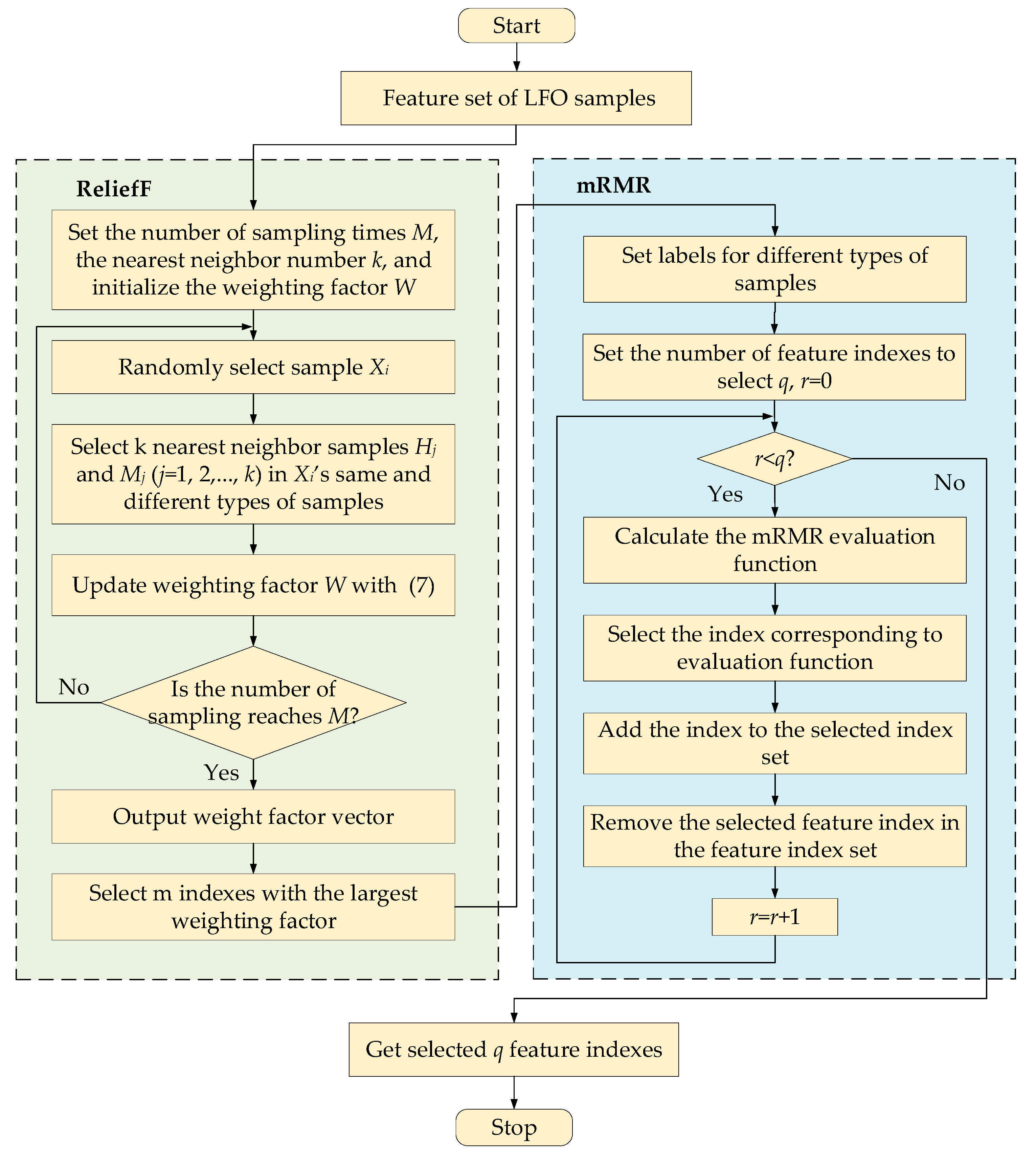
Although ReliefF is simple and efficient, the selected feature subset may be redundant. mRMR algorithm can reduce feature subset redundancy, but it is computationally inefficient in the face of high-dimensional features. Accordingly, ReliefF-mRMR is adopted to select subset features. Firstly, ReliefF selects out M features from entire feature set. Then, mRMR screens out q minimum redundancy maximum relevance features from the features selected by ReliefF. The flow chart of LFO feature subset selection is shown in Figure 1.
4. LFO Type Identification Method Based on Multidimensional Features and ReliefF-mRMR
It is difficult for traditional approaches to identify LFO type by the multidimensional feature subset because they are hard to mine valuable information in mass data. However, SVM has a good generalization ability and can find nonlinear relationships in data, so it has a unique strength for exploring deep relationships between LFO features and types which have not been discovered or are hard to find. Even so, the classification accuracy may not be high in some cases for traditional fixed parameters SVM. In this paper, GA-SVM is adopted, in which genetic algorithm is utilized to optimize SVM parameters, so that training model has a higher classification accuracy. Therefore, the model trained by GA-SVM could discriminate LFO type reliably.
4.1. Principle of GA-SVM
SVM was first proposed by Vapnik in 1963 [28]. It is a supervised learning classifier which is suitable for small samples. Its goal is to find a hyperplane that maximizes the interval between different categories to classify sample data. In order to obtain a high reliable and accurate LFO type identification model, a modified parameter GA-SVM is adopted to train feature subset, which can map linearly inseparable data in low-dimensional space to high-dimensional space by kernel function, making data linearly separable in high-dimensional space. SVM parameters play key roles in classification, but there are no specific approaches of setting traditional SVM parameters. Nevertheless, GA-SVM can overcome the shortcomings of traditional SVM by adopting genetic algorithm to optimize the penalty factor and kernel function parameters, and then a model with the optimal classification ability can be obtained. The genetic algorithm is an artificial intelligence heuristic algorithm that solves the optimization problem. It can effectively avoid falling into local optimum and find global optimal solution through individual evaluation, selection, crossover, mutation, and other operations. Therefore, GA-SVM has a better classification ability than traditional fixed-parameter SVM, and the model trained by GA-SVM also has a higher accuracy.
The hyperplane of SVM can be expressed as
where w is the normal vector of hyperplane, x is eigenvector, and b is the offset between the origin and the hyperplane.
The Gaussian radial basis function (RBF) kernel adopted in this paper is a kind of kernel function with good performance, and the effect of RBF on most classification problems is good. The formula of the Gaussian radial basis kernel function is
where x and x’ are eigenvectors of different samples, ||x-x’|| is the distance between two samples, and σis the width parameter of the Gaussian radial basis kernel function.
4.2. Flow of LFO Type Identification Method Based on Multidimensional Features and ReliefF-mRMR
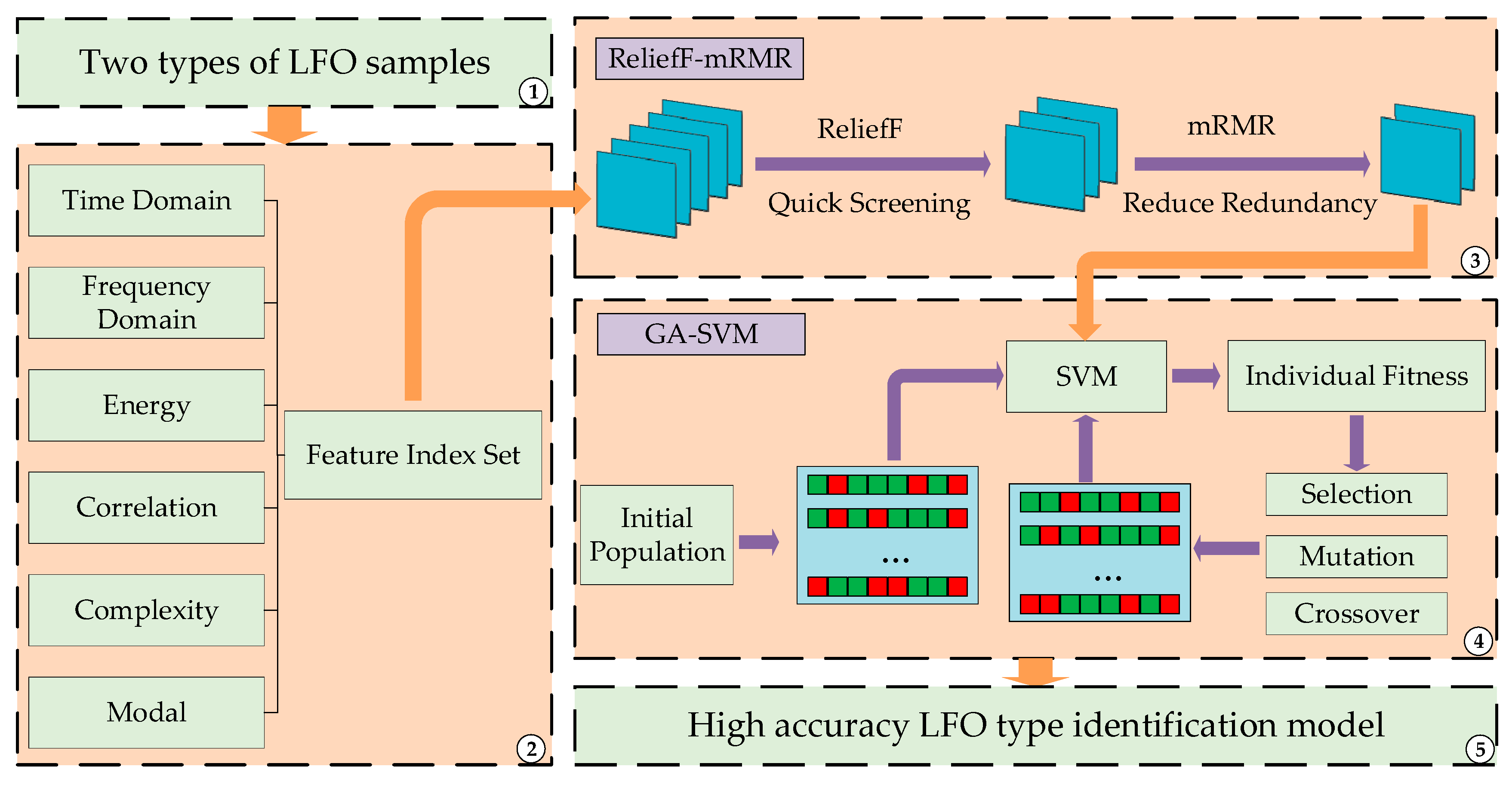
According to Section 3 and Section 4, we can get the flow of the LFO type identification method. The schematic diagram is shown in Figure 2. The specific steps are as follows:
- Obtain actual event samples or simulation samples considering various influencing factors such as disturbance source characteristics, power system operating conditions, damping level, noise, etc.
- Calculate feature index set of samples including time domain, frequency domain, energy, correlation, complexity, and modal analysis.
- Obtain feature subset with ReliefF-mRMR.
- Train LFO type identification model for feature subset with GA-SVM.
- Input feature index set of unknown type LFO data into identification model to identify LFO type.
5. Case Study and Analysis
In this section, considering measurement noise, incomplete recording data, and system damping ratio close to 0, the proposed method is verified in 179-bus system. The simulation model contains 179 buses, 29 generators, and 263 branches including transformers. The rotor motion of each generator is reflected by a classical second-order differential model. The damping parameters of all generators are initially set to 4 and all loads are modeled as a constant load. 28 natural oscillatory modes exist in this system, which range from 0.26~1.88 Hz [29,30]. The method has also proved to be effective with the actual event data happened in ISO New England and East China power system.
5.1. Sample Construction and Model Training
The Power System Analysis Toolbox (PSAT) is used to carry out batch simulation of natural oscillations and forced oscillations, and the simulation time is set to 18 s.
Natural oscillations samples are constructed by adjusting damping parameter of different generators and applying three-phase short-circuit faults at different locations. Table 3 shows the detailed cases description of natural oscillations samples which are created in the modified WECC 179-bus power system. In each case, buses with generators whose damping parameter are modified, are shown in the second column, and the damping parameter of these generators are shown in the third column. ‘NO’ means natural oscillations. In each case of Table 3, a three-phase short circuit that lasts 0.05 s is applied on fault bus, so samples of natural oscillations can be constructed. A series of samples in one case is obtained by increasing the load level from 95% to 105% rated load gradually, and the load changes 0.5% rated load in each step. For natural oscillations events, damping ratios of power system could be negative, close to zero or positive. The cases where damping ratios are close to zero are difficult to identify the type of LFO, because their waveforms are similar to forced oscillations waveforms. In order to improve identification ability of training model in these conditions, the samples in this special case, need to be included into natural oscillations samples. Based on this, NO8–NO15 are the cases with the damping ratio close to zero.
Forced oscillations samples are constructed by applying periodic disturbances to prime mover torques and excitation system inputs of 29 different generators in the system. Table 4 shows the details of the disturbances applied to the generators. The amplitude is the ratio of disturbance to the initial output power of generators. For each generator, the disturbances in Table 4 are applied to torques of prime movers and inputs of excitation systems, and disturbance amplitude step and frequency step are 0.05 and 0.02, respectively. Let the loads vary from 95% to 105% rated load, so the forced oscillations samples are generated by changing the load level when a disturbance is applied to the system.
In order to imitate the obtained PMU data in actual system, measurement noise of which the signal to noise ratio is 50 is applied to both the natural oscillations samples and the forced oscillations samples. Besides, the data sampling frequency is set to 30 Hz, which is widely adopted by the PMUs in actual system [31,32]. The apparent power base of the per unit (pu) is 100 MVA and the generator with the greatest active power fluctuation are selected to calculate the feature index sets, in which the sample entropy parameter m is set to 2, and r is set to 0.15 times the time series standard deviation. The nearest neighbor parameter k of ReliefF algorithm is set to 10, and the number of features mRMR selected q is 5. In order to demonstrate the advantages of ReliefF-mRMR, four methods are used for feature selection, which are ReliefF-mRMR, mRMR, ReilefF, and Pearson correlation coefficient, respectively. Table 5 shows the features selected by the four methods and the identification accuracy of LFO type by training these features with SVM without parameter optimization. The penalty factor ct of traditional SVM is set to 1 and the RBF kernel parameter gt is set to 1.8, 7.3, 28, respectively [33,34]. Then the model with highest accuracy is selected. The reason why SVM without parameter optimization is used here is to highlight the advantages of ReliefF-mRMR, and the features selected by this method have better robustness. The number of selected features is set to 5 and 5-fold cross validation is used to verify the accuracy of four feature selection methods. As can be seen from Table 5, ReliefF-mRMR has the highest accuracy among the four methods, so ReliefF-mRMR is chosen as the feature selection method in this paper. The selected feature subset with ReliefF-mRMR includes kurtosis index of time domain, waveform index of energy function, cross-correlation index, variance of frequency domain, and skewness of frequency domain.
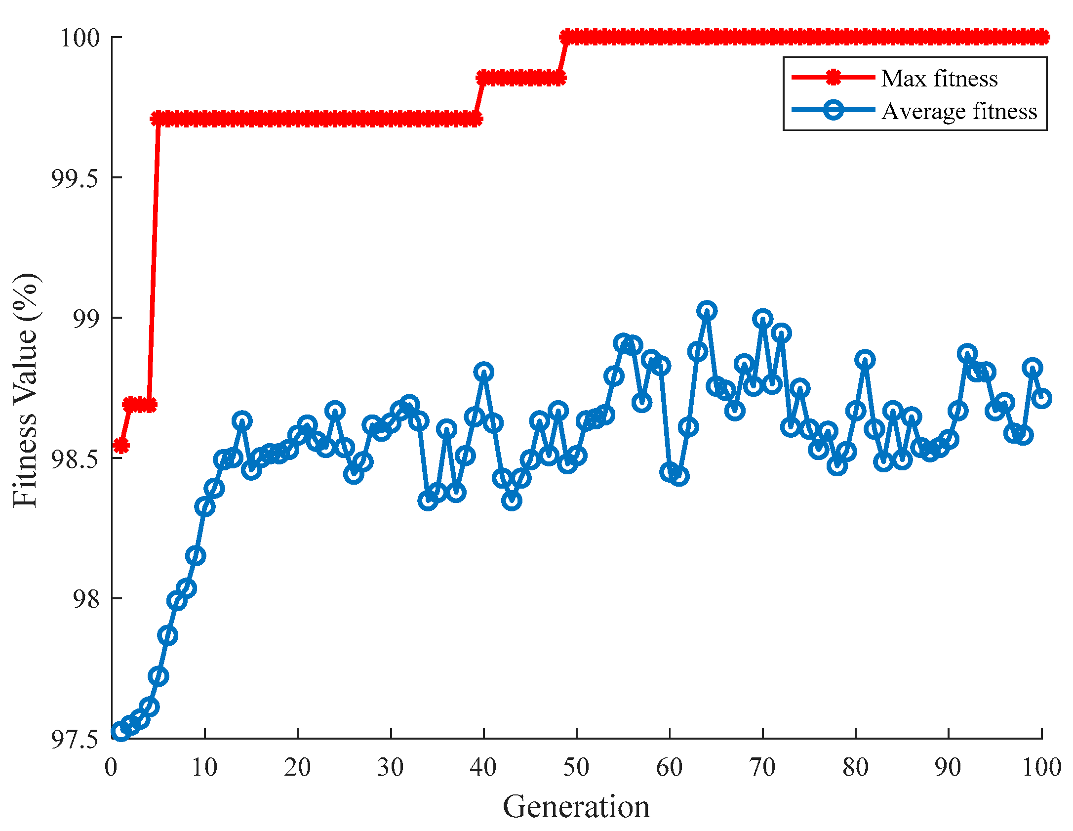
In order to obtain higher accuracy identification model, GA-SVM is adopted to train the training group feature subset. The samples are divided into two groups, and proportions of the test group and training group to the total samples are 85% and 15%, respectively. Set maximum evolution generation to 100 and population to 20. The training model is utilized to identify the LFO type of test group. The accuracy of training model reaches 100%, and the optimized penalty factor co of SVM is 75.1959 and the optimized RBF kernel parameter go is 0.014305. The fitness curve is shown in Figure 3.
5.2. Validation
In this section, the effectiveness of the method is verified for the case that recorded data is incomplete and natural oscillations damping ratio is close to zero.
(a) Recorded data is incomplete
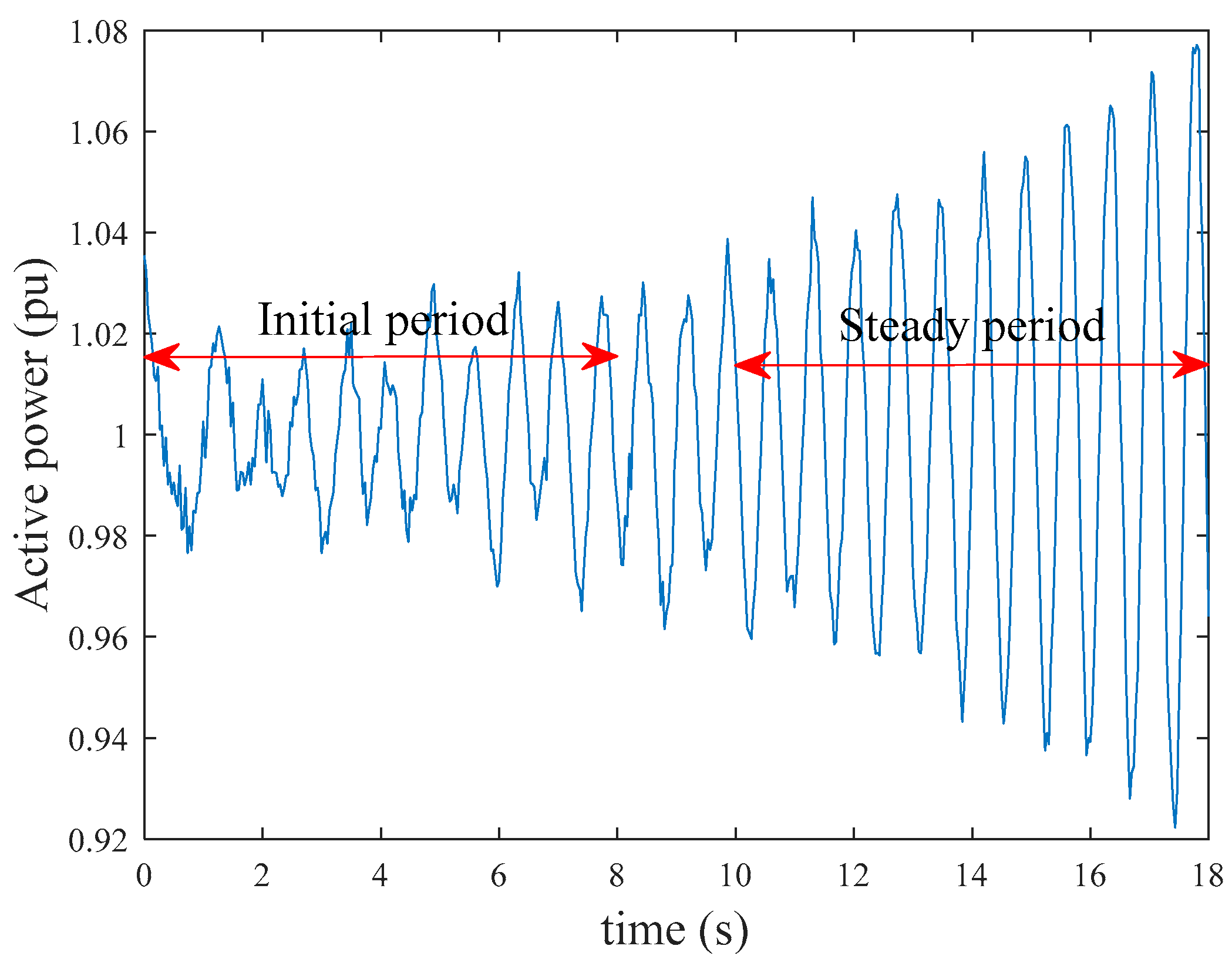
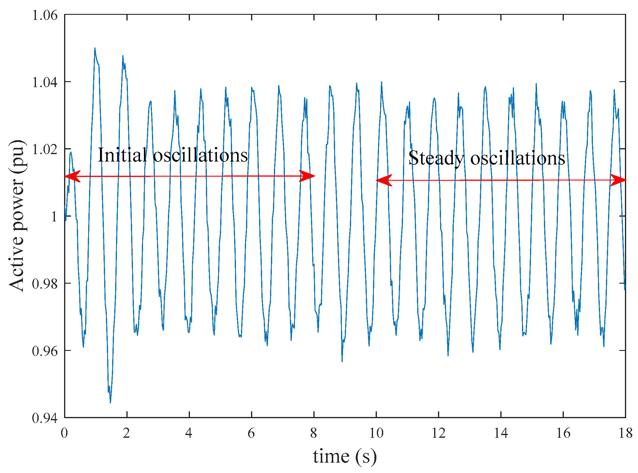
In actual events, the initial period of oscillation may not be recorded which leads to the incompletion of recorded data. Therefore, both the initial period and steady period of LFO wave are tested and the accuracy of the training models are verified.
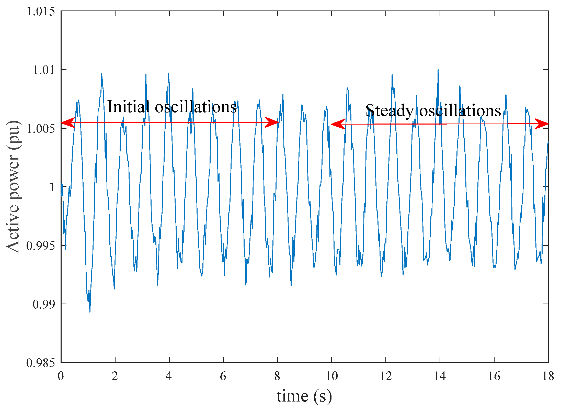
Batch simulation of two types of oscillations are carried out in the 179-bus system. Typical natural oscillations are shown in Figure 4 and typical forced oscillations are shown in Figure 5. The data of 0–8 s is taken as the initial period waveform and the data of 10–18 s is taken as steady period waveform. The oscillations of 0–8 s are termed as ‘initial oscillations’ and the oscillations of 10–18 s are termed as ‘steady oscillations’ in this paper. The reason for this is that the initial period of oscillations contains many components with small time constants, which will attenuate quickly. After these components attenuate, the remained components will sustain for longer time, which are hence considered as the steady oscillations. The training group are trained by SVM without parameter optimization and GA-SVM, respectively. The model accuracy of the LFO type identification models is shown in Table 6. It can be seen that GA-SVM has a higher identification accuracy for the incomplete recording data.
(b) Damping ratio is close to zero
For the case where natural oscillations damping ratio is close to 0, the waveform (as shown in Figure 6) is very similar to the forced oscillations. The feature subset of samples containing the natural oscillations which damping ratio is close to 0 is calculated, and then the training model is utilized to identify the oscillation type. By the test, the method successfully identifies that the oscillation in Figure 6 is natural oscillations.
(c) ISO New England and East China Power Grid
Unlike in small system, the waveforms of LFOs happened in actual large interconnected power systems are often irregular due to the complexity of the power system and the diversity of disturbances. In order to verify the practicability of the proposed method in actual power system, the method is applied to the oscillation data of ISO New England and East China power grid. In addition, to further improve the accuracy of LFO type identification model applied to actual power systems, oscillation data of actual system is also added into the training group to improve the generalization ability of the model.
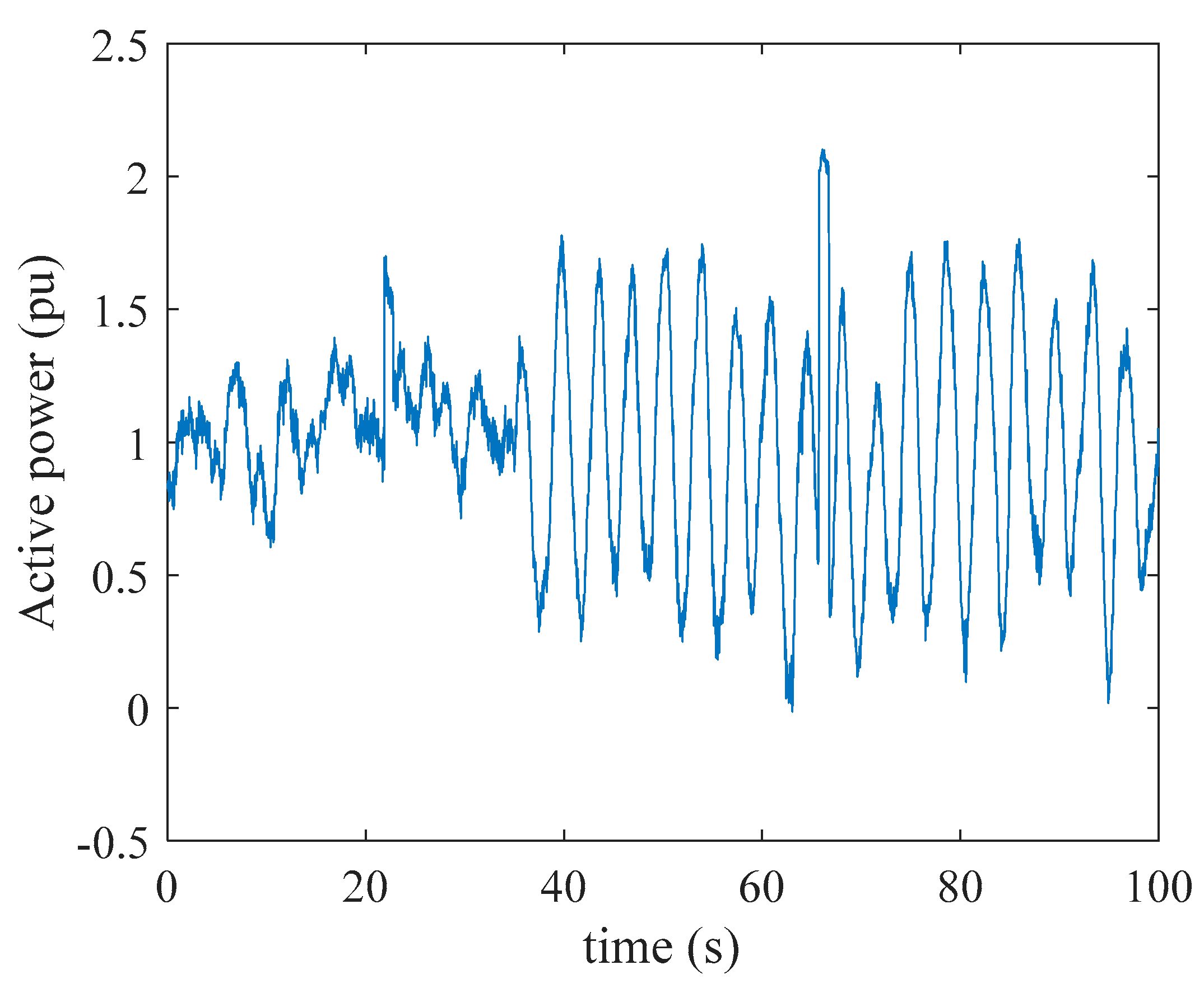
An actual LFOs event shown in Figure 7 is used to validate the applicability of the method. The LFOs happened in New England on 17 June 2016 and its type is forced oscillations [35]. It is a near-resonance condition with a system-wide natural oscillatory mode caused by a large generator. Its peak-to-peak magnitude reaches 27 MW and the frequency is 0.27 Hz. Figure 7 shows that the waveform is relatively stable between 40 s and 80 s, so this period of oscillating data is chosen as an actual sample. The proposed method is applied to the data and the discriminant result is forced oscillations, which is consistent with the actual situation.
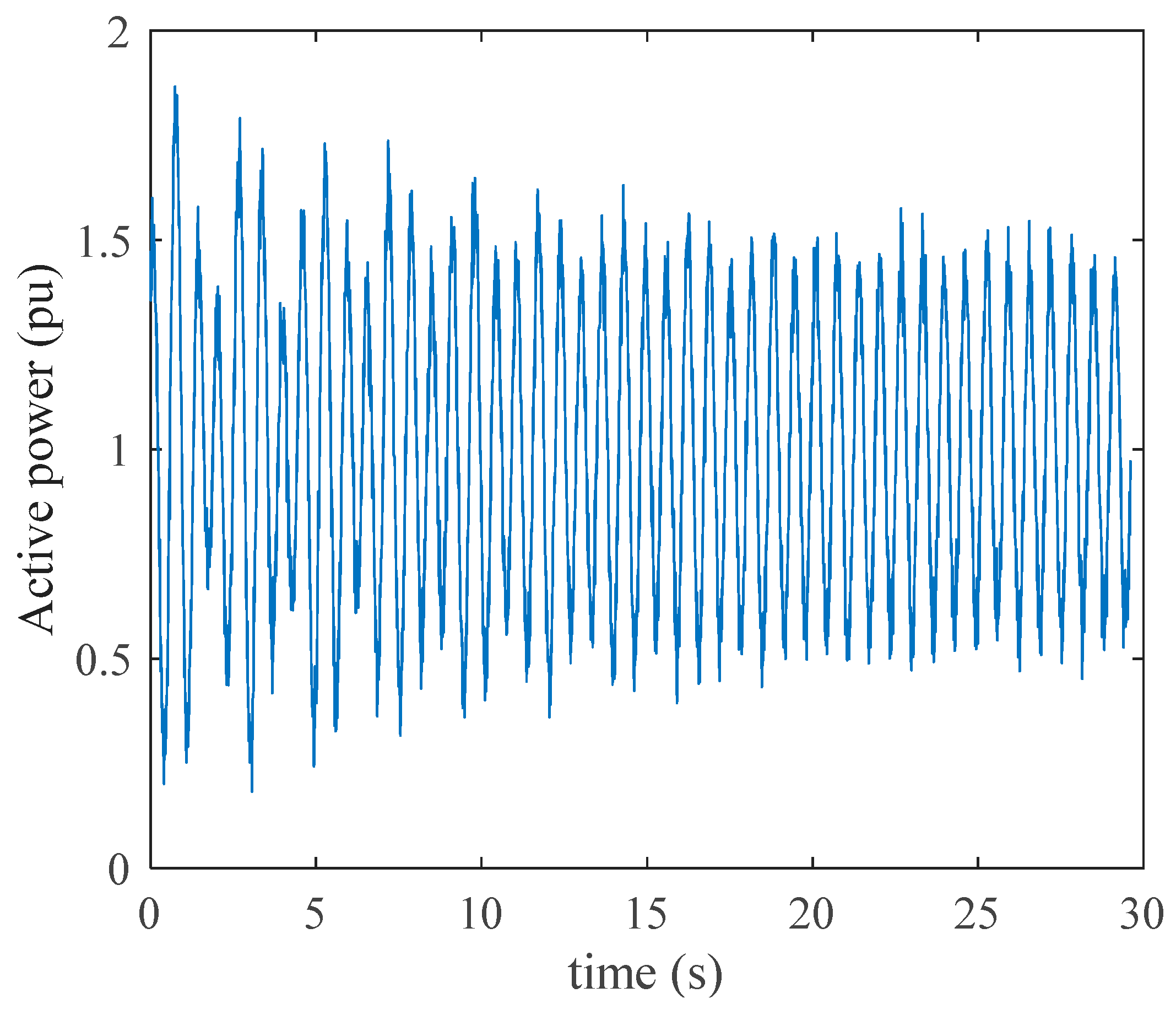
Test cases of natural oscillations and forced oscillations in East China power grid are used to verify the proposed method. A natural oscillations event in East China power grid is shown in Figure 8, and it is the active power of ZTS generator in Zhejiang Province. These natural oscillation events are caused by a three-phase short circuit lasting 0.04 s at bus ZTS in Zhejiang Province. According to small signal stability analysis in East China power grid, ZTS mainly participates in an oscillation mode that the frequency is 1.55 Hz and the damping ratio is 0.001. Besides, the frequency of the oscillation curve in Figure 8 at the steady oscillations state is 1.55 Hz by frequency domain analysis. Therefore, it can be considered that this LFO event is caused by the three-phase short circuit inducing the near-zero oscillation mode. After calculating the feature indexes of the waveform and inputting the feature indexes to the LFO identification model, the discriminant result also shows that this is a natural oscillation event, which is consistent with the actual situation.
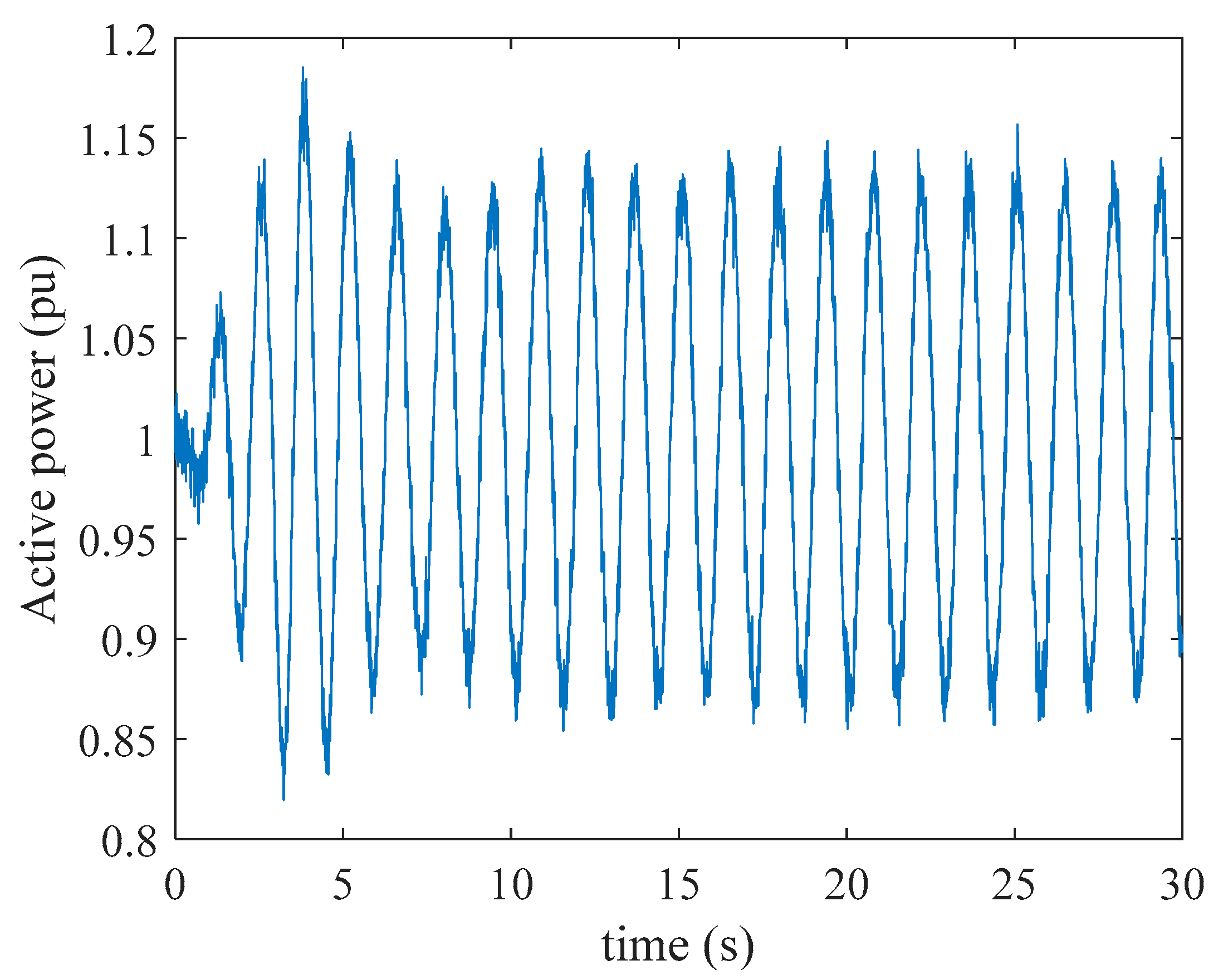
Another forced oscillation event in East China power grid is adopted to verify the proposed method. The forced oscillation event is caused by a sinusoidal disturbance of 0.70 Hz at SHJ generator in Jiangsu Province, since there is an oscillation mode of 0.70 Hz between Jiangsu and Shanghai. Large oscillations of the HXB generator in Shanghai are induced and Figure 9 shows the active power waveform of HXB generator. The maximum oscillation amplitude is about 0.18 pu and the frequency is 0.70 Hz. By applying the proposed method to the oscillations data, the LFO type is identified as forced oscillation, which is in accordance with the actual situation.
6. Conclusions and Future Work
In this paper, the multi-dimensional characteristics of oscillation data are firstly proposed to characterize LFOs. By using ReliefF-mRMR to extract features from oscillating samples and GA-SVM to train the recognition model, the feature subset with minimum redundancy and the model with high identification accuracy can be obtained. In addition to consideration of measurement noise, the training samples with damping ratio close to 0—which are difficult for identifying the type of LFO by previous methods—are also added to enhance the identification accuracy of the oscillation type identification model. Finally, the cases of incomplete data and damping ratio close to 0 are verified, the results indicate that this approach has high robustness and noise immunity. The identification accuracy of the training model is validated with the data of actual power grid. The validation results show that the method has strong practicability.
Future studies can be also further developed for the location of oscillation sources based on proposed method.
Author Contributions
Funding acquisition, S.F.; Investigation, J.C.; Methodology, S.F.; Project administration, Y.T.; Software, J.C.; Supervision, Y.T.; Writing—original draft, J.C.; Writing—review & editing, S.F. and Y.T.
Funding
This research was funded by National Key R&D Program of China grant number 2018YFB0904500 And National Natural Science Foundation of China grant number 51807025.
Conflicts of Interest
The authors declare no conflict of interest.
References
- Feng, S.; Wu, X.; Jiang, P.; Xie, L.; Lei, J.X. Mitigation of Power System Forced Oscillations: An E-STATCOM Approach. IEEE Access 2018, 6, 31599–31608. [Google Scholar] [CrossRef]
- Sui, X.; Tang, Y.; He, H.; Wen, J. Energy-Storage-Based Low-Frequency Oscillation Damping Control Using Particle Swarm Optimization and Heuristic Dynamic Programming. IEEE Trans. Power Syst. 2014, 29, 2539–2548. [Google Scholar] [CrossRef]
- Zhao, Y.; Li, Z.; Nie, Y. A Time-Frequency Analysis Method for Low Frequency Oscillation Signals Using Resonance-Based Sparse Signal Decomposition and a Frequency Slice Wavelet Transform. Energies 2016, 9, 151. [Google Scholar] [CrossRef]
- Zhou, N.; Dagle, J. Initial results in using a self-coherence method for detecting sustained oscillations. In Proceedings of the 2015 IEEE Power & Energy Society General Meeting, Denver, CO, USA, 26–30 July 2015. [Google Scholar]
- Liu, J.; Yao, W.; Wen, J.Y. Active Power Oscillation Property Classification of Electric Power Systems Based on SVM. J. Appl. Math. 2014, 2014, 218647. [Google Scholar] [CrossRef]
- Ma, Y.F.; Liu, W.D.; Zhao, S.Q. On-line identification of low-frequency oscillation properties based on envelop fitting. Autom. Electr. Power Syst. 2014, 38, 46–53. [Google Scholar]
- Ye, H.; Liu, Y.; Zhang, P. Analysis and Detection of Forced Oscillation in Power System. IEEE Trans. Power Syst. 2017, 32, 1149–1160. [Google Scholar] [CrossRef]
- Feng, S.; Jiang, P.; Wu, X. Frequency domain method for identifying property of low frequency oscillations. Proc. Chin. Soc. Electr. Eng. 2016, 36, 2357–2365. [Google Scholar]
- Wang, X.; Turitsyn, K. Data-Driven Diagnostics of Mechanism and Source of Sustained Oscillations. IEEE Trans. Power Syst. 2016, 31, 4036–4046. [Google Scholar] [CrossRef]
- Xie, R.C.; Trudnowski, D. Distinguishing features of natural and forced oscillations. In Proceedings of the 2015 IEEE Power & Energy Society General Meeting, Denver, CO, USA, 26–30 July 2015. [Google Scholar]
- Dai, X.Z.; Shen, C. A power system oscillation property identifying method based on decomposition of energy supply on port. Autom. Electr. Power Syst. 2014, 38, 40–45. [Google Scholar]
- Pai, M.A. Energy Function Analysis for Power System Stability; Kluwer Academic Publishers: Boston, MA, USA, 1989; pp. 1–48. [Google Scholar]
- Fouad, A.A.; Vittal, V. Power System Transient Stability Analysis: Using the Transient Energy Function Method; Prentice-Hall: Englewood Cliffs, NJ, USA, 1991. [Google Scholar]
- Tsolas, N.; Arapostathis, A.; Varaiya, P. A structure preserving energy function for power system transient stability analysis. IEEE Trans. Circuits Syst. 1985, 32, 1041–1049. [Google Scholar] [CrossRef]
- Moon, Y.H.; Cho, B.H.; Lee, Y.H.; Hong, H.S. Energy conservation law and its application for the direct energy method of power system stability. In Proceedings of the IEEE Power Engineering Society, 1999 Winter Meeting (Cat. No.99CH36233), New York, NY, USA, 31 January–4 February 1999. [Google Scholar]
- Min, Y.; Chen, L. A transient energy function for power systems including the induction motor model. Sci. China Ser. E 2007, 5, 575–584. [Google Scholar] [CrossRef]
- Chen, L.; Min, Y.; Chen, Y.P.; Hu, W. Evaluation of Generator Damping Using Oscillation Energy Dissipation and the Connection with Modal Analysis. IEEE Trans. Power Syst. 2014, 29, 1393–1402. [Google Scholar] [CrossRef]
- Chen, L.; Sun, M.; Min, Y.; Xu, X.L.; Xi, J.H.; Li, Y. Online monitoring of generator damping using dissipation energy flow computed from ambient data. IET Gener. Transm. Distrib. 2017, 18, 4430–4435. [Google Scholar] [CrossRef]
- Haque, M.H. Use of energy function to evaluate the additional damping provided by a STATCOM. Electr. Power Syst. Res. 2004, 72, 195–202. [Google Scholar] [CrossRef]
- Chen, L.; Min, Y.; Hu, W. An energy-based method for location of power system oscillation source. IEEE Trans. Power Syst. 2013, 28, 828–836. [Google Scholar] [CrossRef]
- Zhang, X.H.; Zhang, W.C.; Xi, J.H. Discrimination Method for Low-frequency Oscillation Type Based on Entropy of Energy Distribution in Space and Time. Autom. Electr. Power Syst. 2017, 41, 84–90. [Google Scholar]
- Wang, Y.R.; Wu, T.X. Vibration Signal Extraction of Rotating Machines Based on the Analysis of Degree of Cylcostationary. Adv. Mater. Res. 2012, 546, 188–193. [Google Scholar] [CrossRef]
- Hoshino, K.; Sumi, H.; Nishimura, T. Noise Detection and Reduction for Image Sensor by Time Domain Autocorrelation Function Method. In Proceedings of the 2007 IEEE International Symposium on Industrial Electronics, Vigo, Spain, 4–7 June 2007. [Google Scholar]
- Yan, R.; Gao, R.X. Approximate Entropy as a diagnostic tool for machine health monitoring. Mech. Syst. Signal Process. 2007, 21, 824–839. [Google Scholar] [CrossRef]
- Kononenko, I.; Šimec, E.; Robnik-Šikonja, M. Overcoming the Myopia of Inductive Learning Algorithms with RELIEFF. Appl. Intell. 1997, 7, 39–55. [Google Scholar] [CrossRef]
- Kwak, N.; Choi, C.H. Input feature selection by mutual information based on Parzen window. IEEE Trans. Pattern Anal. Mach. Intell. 2002, 24, 1667–1671. [Google Scholar] [CrossRef] [Green Version]
- Peng, H.C.; Long, F.H.; Ding, C. Feature selection based on mutual information criteria of max-dependency, max-relevance, and min-redundancy. IEEE Trans. Pattern Anal. Mach. Intell. 2005, 27, 1226–1238. [Google Scholar] [CrossRef]
- Vapnik, V.N. Statistical Learning Theory; John Wiley & Sons: New York, NY, USA, 1998. [Google Scholar]
- Maslennikov, S.; Wang, B.; Zhang, Q.; Ma, F.; Luo, X.; Sun, K.; Litvinov, E. A test cases library for methods locating the sources of sustained oscillations. In Proceedings of the 2016 IEEE Power and Energy Society General Meeting, Boston, MA, USA, 17–21 July 2016. [Google Scholar]
- Chevalier, S.; Vorobev, P.; Turitsyn, K. A Bayesian Approach to Forced Oscillation Source Location Given Uncertain Generator Parameters. IEEE Trans. Power Syst. 2019, 34, 1641–1649. [Google Scholar] [CrossRef]
- Follum, J.; Pierre, J.W. Detection of Periodic Forced Oscillations in Power Systems. IEEE Trans. Power Syst. 2016, 31, 2423–2433. [Google Scholar] [CrossRef]
- Khan, M.A.; Pierre, J.W. Detection of Periodic Forced Oscillations in Power Systems Using Multitaper Approach. IEEE Trans. Power Syst. 2019, 34, 1086–1094. [Google Scholar] [CrossRef]
- Christianini, N.; Shawe-Taylor, J. An Introduction to Support Vector Machines and Other Kernel-Based Learning Methods; Cambridge University Press: Cambridge, UK, 2000. [Google Scholar]
- Trevor, H.; Robert, T.; Jerome, F. The Elements of Statistical Learning, 2nd ed.; Springer: New York, NY, USA, 2008. [Google Scholar]
- CURENT: Test Cases. Available online: http://web.eecs.utk.edu/~kaisun/Oscillation/actualcases.html (accessed on 12 May 2019).
Figure 1.
Flow chart of LFO feature subset selection based on ReliefF-mRMR.

Figure 2.
Schematic diagram of LFO type identification method based on multidimensional features and ReliefF-mRMR.
Figure 2.
Schematic diagram of LFO type identification method based on multidimensional features and ReliefF-mRMR.

Figure 3.
Fitness curve of GA optimizing parameters, and the identification accuracy reaches nearly 100% after 49 generations.
Figure 3.
Fitness curve of GA optimizing parameters, and the identification accuracy reaches nearly 100% after 49 generations.

Figure 4.
Typical natural oscillations waveform.

Figure 5.
Typical forced oscillations waveform.

Figure 6.
Natural oscillations with damping ratio close to zero.

Figure 7.
Forced oscillations with the frequency of 0.27 Hz in ISO New England, which are successfully identified as forced oscillations by the proposed method.
Figure 7.
Forced oscillations with the frequency of 0.27 Hz in ISO New England, which are successfully identified as forced oscillations by the proposed method.

Figure 8.
Active power oscillation with the frequency of 1.55 Hz of ZTS generator in Zhejiang Province, which is successfully identified as natural oscillation by the proposed method.
Figure 8.
Active power oscillation with the frequency of 1.55 Hz of ZTS generator in Zhejiang Province, which is successfully identified as natural oscillation by the proposed method.

Figure 9.
Active power oscillation with the frequency of 0.70 Hz of HXB generator in Shanghai, which is successfully identified as a forced oscillation by the proposed method.
Figure 9.
Active power oscillation with the frequency of 0.70 Hz of HXB generator in Shanghai, which is successfully identified as a forced oscillation by the proposed method.


Table 1.
Time domain feature indexes.
| Expression | Meaning |
|---|---|
| Mean | |
| Standard deviation | |
| Square root amplitude | |
| Root mean square value (effective value) | |
| Peak | |
| Twist index (skewed indicator) | |
| Kurtosis index | |
| Crest factor | |
| Margin index | |
| Waveform index | |
| Pulse index |
where x(n) is the signal sequence (n = 1, 2, …, N), and N is the number of sampling points.
Table 2.
Frequency domain feature indexes.
| Expression | Meaning |
|---|---|
| Center frequency | |
| variance | |
| Skewness | |
| Kurtosis | |
| Frequency center | |
| Frequency standard deviation | |
| Root mean square frequency | |
| Waveform stability factor | |
| Coefficient of variation | |
| Twist | |
| Kurtosis | |
| Root mean square ratio |
where s(k) is the spectrum of the signal (k = 1, 2, ..., K), K is the number of spectral lines, and fk is the frequency of the k-th spectral line.
Table 3.
Cases of natural oscillations.
| Case Number | Buses of Generators with Modified Parameter | Damping Parameter | Fault Bus |
|---|---|---|---|
| NO1 | 6, 11 | 2, −6 | 30 |
| NO2 | 6, 11 | 5, −9 | 6 |
| NO3 | 6, 11 | 3, −8 | 30 |
| NO4 | 45, 159 | −2, −0.5 | 159 |
| NO5 | 45, 159 | −0.5, −0.5 | 159 |
| NO6 | 45, 159, 36 | −2.5, 1, −1 | 159 |
| NO7 | 11 | −10 | 79 |
| NO8 | 35, 65 | 0.5, −1.5 | 79 |
| NO9 | 45, 159 | −2, 1 | 159 |
| NO10 | 6, 11 | 1.5, −6 | 30 |
| NO11 | 6, 11 | 5, −8 | 6 |
| NO12 | 6, 11 | 3, −7 | 30 |
| NO13 | 45, 159 | −0.2, −0.2 | 159 |
| NO14 | 45, 159, 36 | −2.5, 1.3, −0.6 | 159 |
| NO15 | 11 | −7.5 | 79 |
Table 4.
Disturbances of forced oscillations.
| Inputs of Disturbance | Wave Form | Amplitude | Frequency (Hz) |
|---|---|---|---|
| Prime mover torque | Sine and square | 0.1–0.5 | 0.2–2.5 |
| Excitation system inputs | Sine and square | 0.05–0.25 | 0.2–2.5 |
Table 5.
Identification accuracy of different feature selection methods.
| Feature Selection Algorithm | Accuracy |
|---|---|
| ReilefF-mRMR | 98.0% |
| mRMR | 95.6% |
| ReilefF | 97.1% |
| Pearson correlation coefficient | 96.9% |
Table 6.
Model identification accuracy.
| Type of Recorded Data | Traditional SVM Accuracy | GA-SVM Accuracy |
|---|---|---|
| Initial period | 94% | 100% |
| Steady period | 92% | 99% |
© 2019 by the authors. Licensee MDPI, Basel, Switzerland. This article is an open access article distributed under the terms and conditions of the Creative Commons Attribution (CC BY) license (http://creativecommons.org/licenses/by/4.0/).
Share and Cite
MDPI and ACS Style
Feng, S.; Chen, J.; Tang, Y. Identification of Low Frequency Oscillations Based on Multidimensional Features and ReliefF-mRMR. Energies 2019, 12, 2762. https://doi.org/10.3390/en12142762
AMA Style
Feng S, Chen J, Tang Y. Identification of Low Frequency Oscillations Based on Multidimensional Features and ReliefF-mRMR. Energies. 2019; 12(14):2762. https://doi.org/10.3390/en12142762
Chicago/Turabian StyleFeng, Shuang, Jianing Chen, and Yi Tang. 2019. "Identification of Low Frequency Oscillations Based on Multidimensional Features and ReliefF-mRMR" Energies 12, no. 14: 2762. https://doi.org/10.3390/en12142762
Note that from the first issue of 2016, this journal uses article numbers instead of page numbers. See further details here.