Validation of a Model for Estimating the Strength of a Vortex Created from the Bound Circulation of a Vortex Generator

Abstract

A hypothesis was tested and validated for predicting the vortex strength induced by a vortex generator in wall-bounded flow by combining the knowledge of the Vortex Generator (VG) geometry and the approaching boundary layer velocity distribution. In this paper, the spanwise distribution of bound circulation on a vortex generator was computed by integrating the pressure force along the VG height, calculated using Computational Fluid Dynamics (CFD). It was then assumed that all this bound circulation was shed into a wake to fulfill Helmholtz’s theorem which then curls up into one primary tip vortex. To validate this, the trailed circulation estimated from the distribution of the bound circulation was compared to the one in the wake behind the vortex generator, determined directly from the wake velocities at some downstream distance. In practical situations, the pressure distribution on a vane is unknown and consequently other estimates of the spanwise force distribution on a VG must instead be applied, such as using 2D airfoil data corresponding to the VG geometry at each wall-normal distance. Such models have previously been proposed and used as an engineering tool to aid preliminary VG design. Therefore, it is not the purpose of this paper to refine such engineering models, but rather to validate their assumptions, such as applying a lifting line model on a VG that has a very low aspect ratio and is placed in a wall boundary layer. Herein, high Reynolds number boundary layer measurements of VG-induced flow were used to validate the Reynolds-Averaged Navier–Stokes (RANS) model circulation results, which were used for further illustration and validation of the hypothesis.

1. Introduction

Vortex generators (VGs), as first described by Taylor in the late 1940s [1,2,3], were originally used to suppress flow separation in diffusors but are today commonly used aerodynamic devices in wind turbine blades, mainly to delay separation at high angles of attack. This increases the maximum lift coefficient and, thus, reduces the necessary chord for the same lift, resulting in more slender and cost-effective blades [4]. VGs are also common in heat exchangers [5], solar receivers [6], thermoelectric power generators [7], and even in microchannels with nanofluids [8], to name a few examples.

VGs in principle consist of small vanes, typically with a triangular or rectangular geometry. They are mounted in the boundary layer with an angle of incidence to the incoming flow that creates vortices behind the VGs causing momentum exchange between the region near the wall and the outer parts of the boundary layer [1,2,3]. Therefore, the boundary layer becomes more resistant to flow reversal in adverse pressure gradients.

The flow behind VGs was investigated experimentally using Particle Image Velocimetry (PIV), in Velte et al. [9] and it was shown that the generated primary vortices possess helical symmetry within a specific range of device angles. Many engineering-based models have been proposed over the years for predicting the primary (tip) vortex circulation, see e.g., [10,11,12,13,14,15]. The models are typically of a design where the circulation would be proportional to the product between the vortex generator height and the average streamwise velocity at the upper tip of the vortex generator. However, these kinds of models typically do not take the variable vortex generator geometry and boundary layer profile into consideration. Furthermore, it has been observed that the occurrence of secondary vortices (from spanwise boundary layer separation and the roll-up effect around the vane base) can substantially affect the circulation of the primary vortex [16]. A more correct manner to obtain the true primary vortex strength (circulation) is, thus, hypothesized to be possible through the integration of the bound vorticity, which was previously tested in [17].

Further, the generated flow can be investigated through the use of Computational Fluid Dynamics modeling. A widely used method is the so-called BAY model [18], where body forces acting on the air near the VGs are specified to induce a realistic flow-field. However, a numerical model that directly resolves the VG geometry should be more accurate, since no prior assumptions on the body forces are required, for example, as has been done in [19], and the results have shown some success compared to both experiments and the BAY model.

In the current work, CFD simulations were performed on a spanwise row of rectangular and triangular VGs. The objective was to test the hypothesis that the strength of the produced vortex responsible for the mixing, quantified as the circulation, Γ, could be calculated from the distribution of the bound circulation along the span of the VG. The local bound circulation was determined from the local sectional lift. The circulation of the streamwise vortex could also be directly computed from the flow-field behind the VG with the direct use of its definition and with the use of the Lamb–Oseen Vortex (LOV). This was then compared to the one estimated from the bound circulation distribution and if this hypothesis was valid, then it would be possible to use this information in preliminary VG designs.

2. Methods

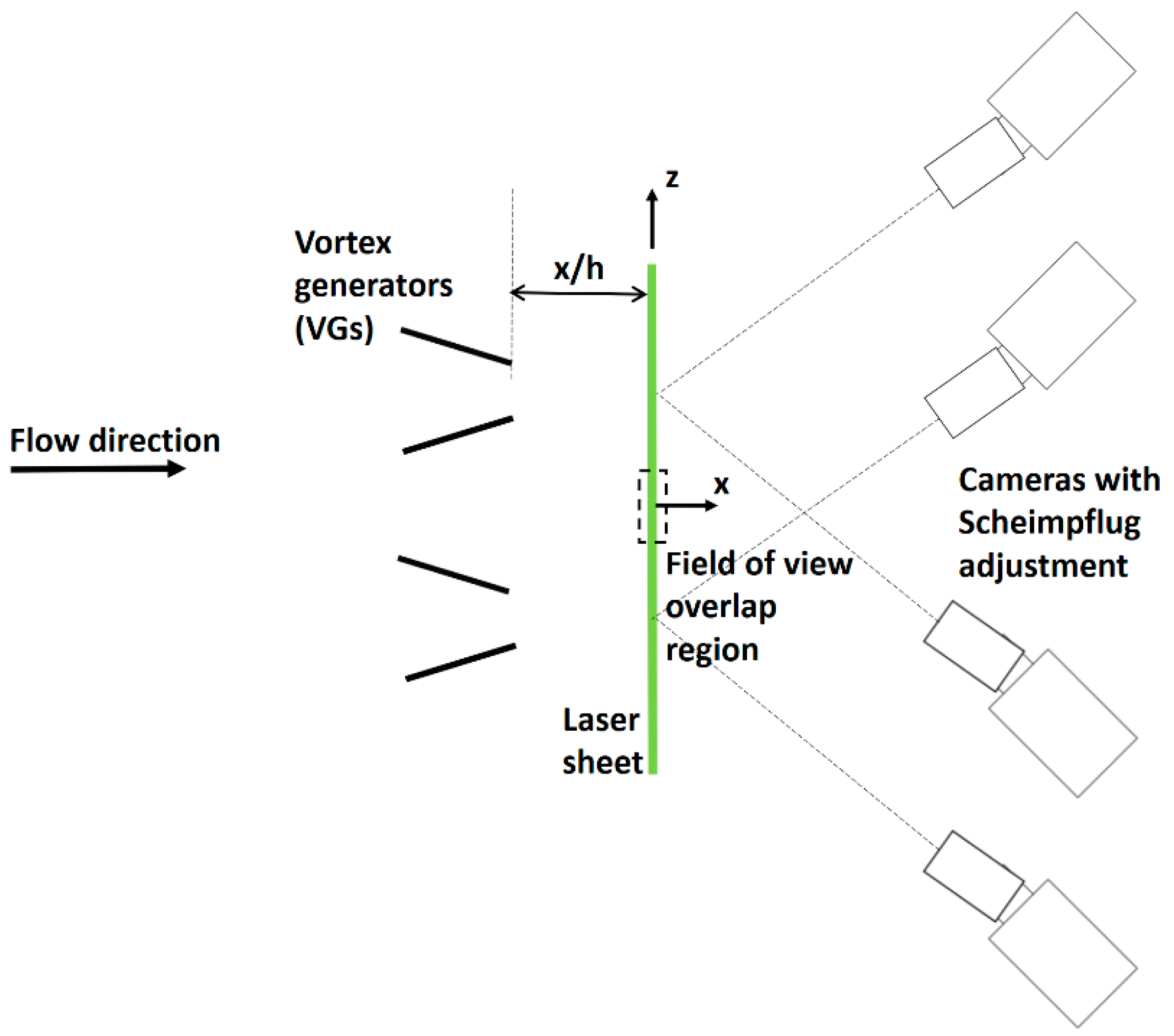
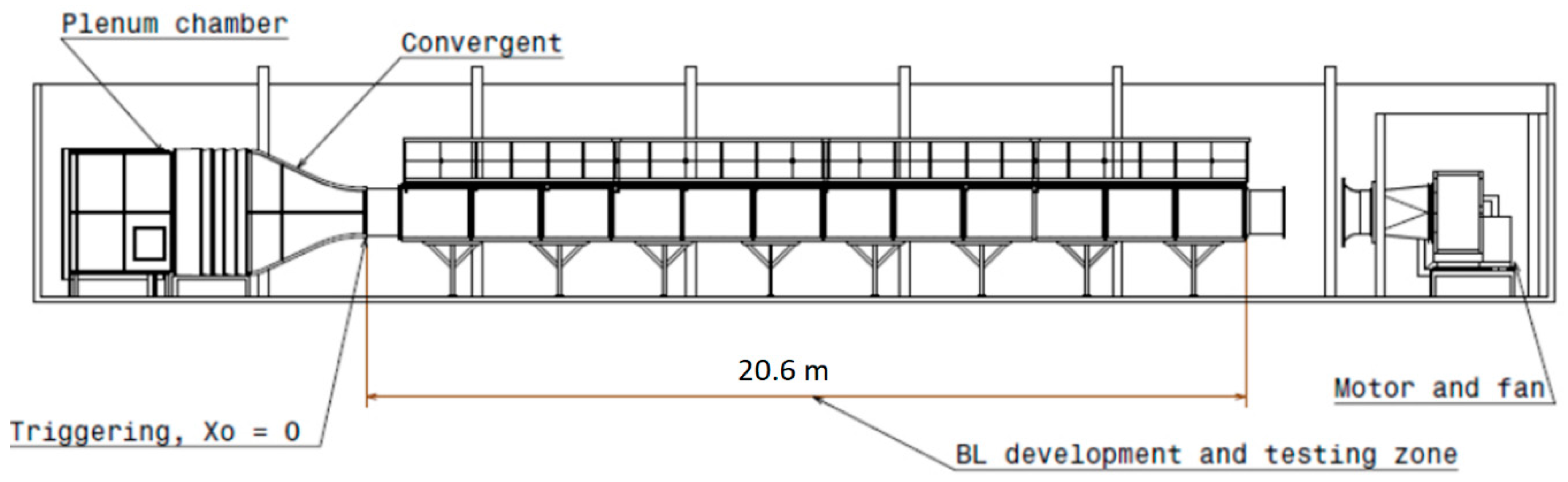
2.1. Experimental Setup

The measurements were carried out in the high Reynolds number wind tunnel in the Laboratoire de Mécanique des Fluides de Lille (LMFL) wind tunnel facility, see Figure 1. This wind tunnel was designed to generate a fully developed turbulent boundary layer with a thickness of δ = 30 cm inside the 20 m long test section. The resulting Reynolds number based on the momentum thickness was 17,000. The large dimensions of the boundary layer allowed for a high effective resolution of the studied flow scales, as well as matching of the Reynolds number to that of VG generated flows on actual wind turbine blades, Re_h = U_∞h/ν = 8.5 ms⁻¹ × 0.06 m/15 × 10⁻⁶ m²s⁻¹ = 34,000, where U_∞ = 8.5 ms⁻¹ was the freestream velocity and h = 0.06 m was the VG height.

Passive VGs of triangular and rectangular shape, respectively, were introduced into the boundary layer at a stage where the boundary layer of 30 cm thickness only developed at a rate of 1 mm per meter, in the downstream direction. Both VG geometries were of height h = 60 mm and length l = 2h = 120 mm and were mounted with an angle of incidence of 18° to the incoming mean flow direction. A top-view of the configuration is illustrated in Figure 2, where L = 2.5h is the distance between the trailing edges in a VG pair and λ = 6h is the spanwise period. This geometric setting that produced counter-rotating vortices was identical for the triangular and rectangular VG experiment configurations.

The flow was imaged in a cross-plane using laser sheet illuminating smoke particles that could faithfully trace the flow, see Figure 3. The laser used was a BMI YAG laser with dual cavities, producing energies of 220 mJ per pulse at 12 Hz repetition frequency. The light sheet was introduced from above. A mirror below the transparent bottom wall, where the VGs were mounted, was used to further utilize the light intensity from the widely spread laser sheet. The beam waist was located approximately at the wall, with a width of approximately 1 mm (measured from burning paper). Furthermore, the light sheets of the two laser pulses were separated by approximately 1.5 mm in the downstream direction, to increase the dynamic range of the measured velocities. The seeding consisted of polyethylene glycol particles with a diameter of the order of 1 µm. This plane was located at variable distances x/h downstream of the VGs. The setup also consisted of four Hamamatsu 2k × 2k pixel cameras equipped with Nikkor 105 mm lenses at f# 5.6. The cameras were at a 45° angle to the light sheet and were, therefore, also equipped with adjustable Scheimpflug mounts that were adjusted accordingly.

The cameras were arranged as two separate stereoscopic PIV setups, where each field of view covered one pair of vortex generators and the fields were ensured to be slightly overlapping to be able to merge the fields into a common wide field of view of about 72 × 28 cm² (corresponding to approximately 2.3 δ × δ) [20,21]. The cameras were placed outside the wind-tunnel.

To extract velocity fields from the images, the in-house PIV processing code of LMFL was employed. The image processing was conducted over an interrogation area size of 24 × 32 pixels with an overlap of 60%, where the non-uniform aspect ratio stemmed from the stretching of the field from the camera perspective angle. In the processing, the self-correction of the calibration due to misalignment between the calibration target and the light sheet was properly accounted for and was self-corrected. The spacing between the interrogation areas after processing was 2 mm, corresponding to 40 wall units. The accuracy of the resulting velocity measurements was thoroughly analyzed in [21], yielding approximately 3% for y/δ larger than approximately 0.1 and not exceeding approximately 12% in the near-wall region across all three velocity components.

An example of the ensemble averaged three-component velocity field measured downstream of the triangular vanes can be seen in Figure 4.

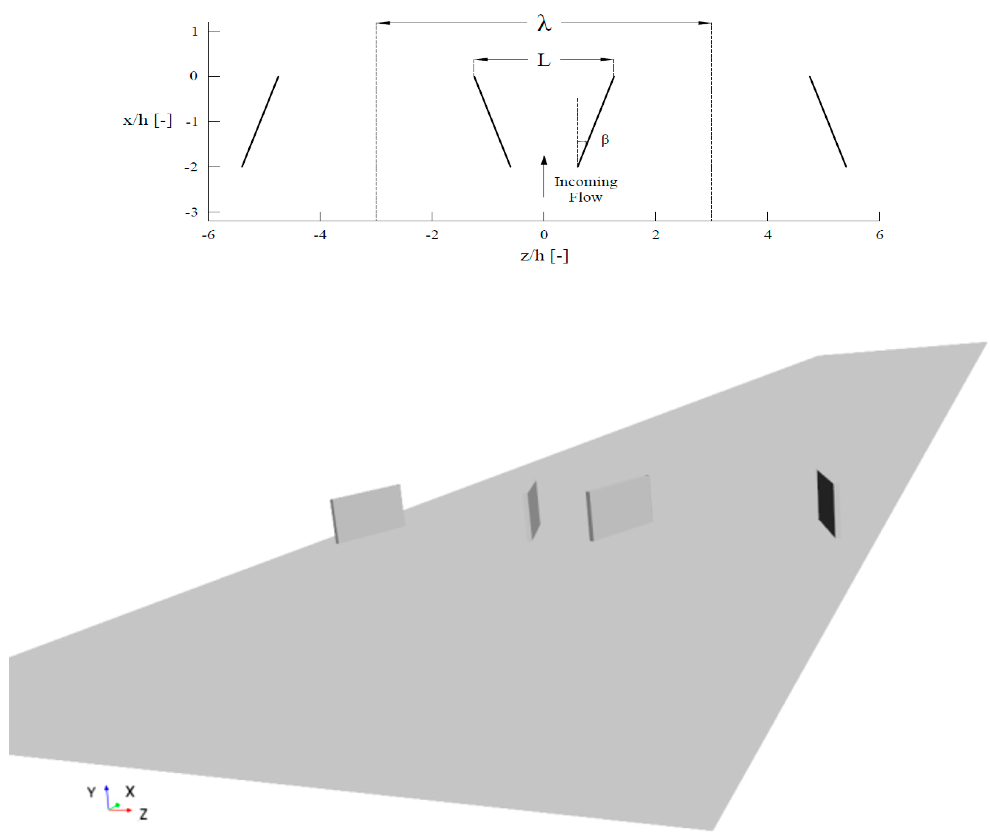
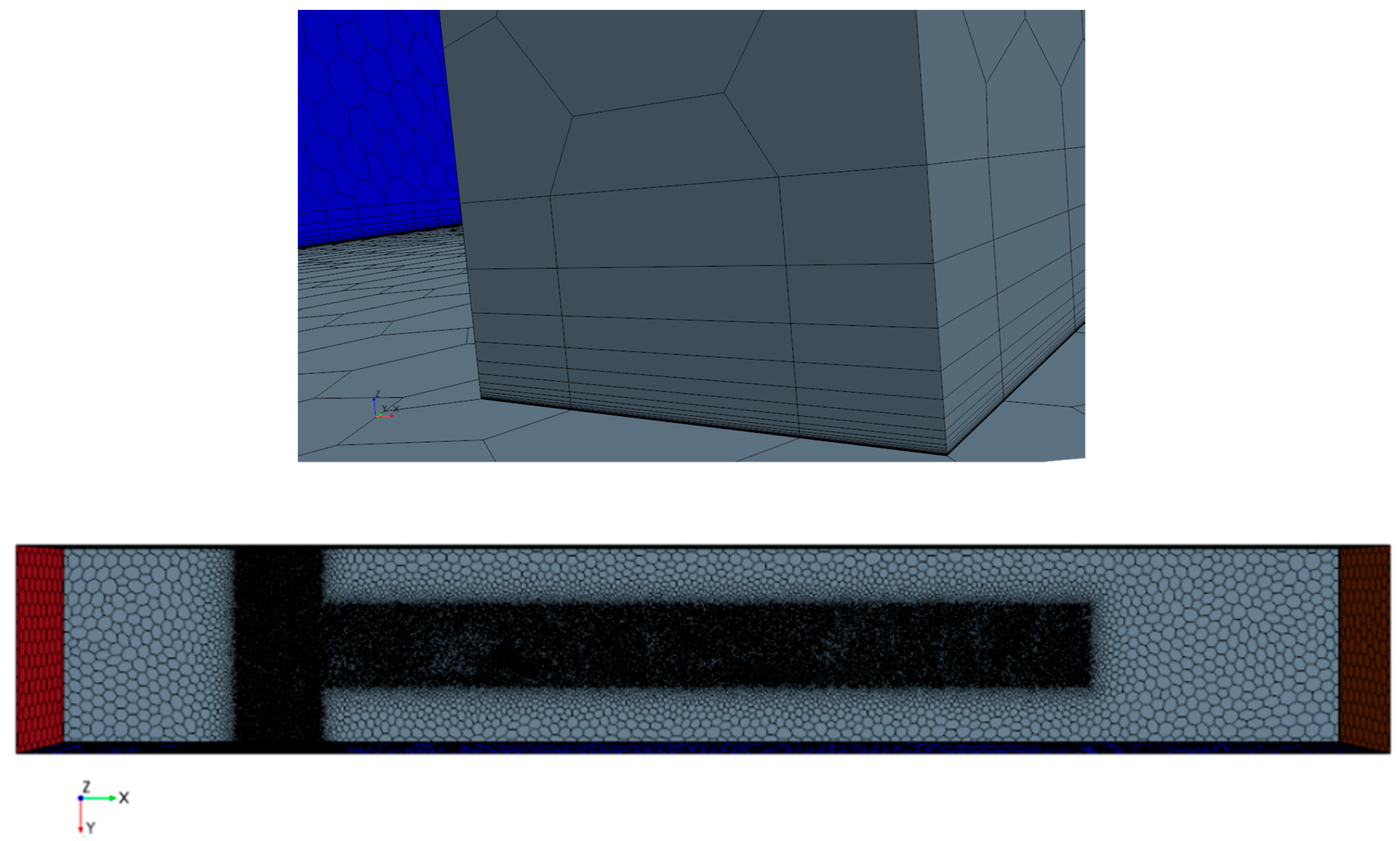
2.2. Numerical Model

Based on the experimental setup presented in [20,21], two RANS models and a Reynold stress model that fully resolved the rectangular and triangular VGs geometries were developed, using the commercial software STAR CM+ [22]. The geometry parts were created and assembled within the software environment with the use of the integrated CAD tool. The authors’ previous experience on modeling vortex generators with models of varying degrees of complexity motivated the inclusion of the Reynolds stress model [23,24].

The tunnel free-stream velocity U was set to 8 m/s as the inlet condition. The distance between the velocity inlet boundary condition and VG leading edges was set to 3.72 m. A parametric analysis using various lengths was conducted for the selection of this value, ensuring a satisfying development of the velocity profile and noting that the VGs were placed deeply inside the boundary layer. The distance between the trailing edges and the rear downstream plane where a pressure outlet boundary condition was applied, was set equal to 3.2 m. This distance was chosen so that the flow did not reverse on the pressure outlet, as the flow in the wake was undisturbed. The distance between the symmetry plane boundary conditions and the trailing edges was 0.075 m, i.e., half the distance between the trailing edges of the middle VG pair (see Figure 2). The height of the computational domain was set equal to 0.4 m. The VGs, as well as the horizontal plane where the vanes were mounted, were treated as the wall boundaries.

The Turbulence Intensity was specified as 1% and the Turbulence Viscosity Ratio was equal to 10. The mesh discretization was 11.3 × 10⁶ and 8.2 × 10⁶ polyhedral cells for the rectangular and triangular set-ups, respectively. The polyhedral meshing option was chosen, since it provides a detailed and balanced solution for complicated studies. Further, it requires lesser computational power since it generates five times fewer cells than the equivalent tetrahedral. Another advantage was that it does not require more surface preparation [22]. The characteristic dimension called the Base size was set equal to 0.05 m for generating the mesh discretization of the overall domain. Specifically, for the rectangular configuration, two relative sizes were chosen for refining the areas that required a detailed resolution. A relative size was chosen for discretizing the region close to the VGs and a second refined region was modeled for capturing the far wake region. A different approach was implemented for discretizing the triangular geometry.

Only the area close to the VGs was refined, since the experimental data used for the validation of the triangular model existed only for 12h downstream, in the planes of the VGs. For the rectangular configuration, the validation sections were up to 50h downstream (i.e., further along the wake). Twenty prism layers were attached near the boundaries for enhanced capturing of the boundary layer development. An illustration of these layers implemented in the rectangular VGs can be seen in Figure 5 (top). The final mesh discretization of the rectangular VGs model can be seen in Figure 5 (bottom). An overview of the parameters used to generate the two grids is presented in

Table 1. Parameters used for the mesh discretization of the rectangular and triangular VGs.

Polyhedral Mesh	Rectangular	Triangular
Base size [m]	0.05	0.05
Relative size close to VGs [%]	9
Relative size in the wake region [%]	11	-
Prism layer mesh	ReD	TrD
Number of prism layers	20	20
Prism layer stretching	1.5	1.5
Prism layer thickness [% of the base size]	5	5
Total amount of cells	11.3 × 106	8.2 × 106

below.

Due to the symmetry of the configuration, the downstream region behind the middle pair was the only one refined in detail, as seen in Figure 5. This practice significantly reduced the computational time and allowed to achieve the highest discretization in the confined area. A sensitivity analysis was carried out for achieving the optimum quality of the mesh discretization, given the computational resources. It was observed that the solutions remained almost unchanged when the discretization was slightly improved by applying lower relative sizes, compared to the aforementioned. However, the main reason for avoiding lower values compared to the values presented in Table 1 is the significant increase in computational time

The three Transport Turbulence Models used to close the RANS equations were Reynolds-Stress, k-ω SST, and Spalart–Allmaras. The solution converge criteria were set to 4000 iteration steps with a tolerance limit equal to 1 × 10⁻⁶. The convergence of the solution was also verified by monitoring the behavior of the residuals. For the rectangular configuration, the residuals reached the tolerance limit and remained almost constant after the first 2000 iteration steps, while for the triangular set-up 1200 iteration steps were needed to meet the same limit.

To validate the accuracy of the numerical models, the results were compared quantitatively with the experimental results, using the circulation of the velocity fields as an indicator. For the y+ values on the VG surface using the Reynolds Stress model, which was the one used for the final comparison, the results varied between 3 and 10, lowest at the leading edge and increasing towards the trailing edge. The circulation was estimated with the direct use of path integration (Equation (8)) and the Lamb-Oseen Vortex (Equation (7)).

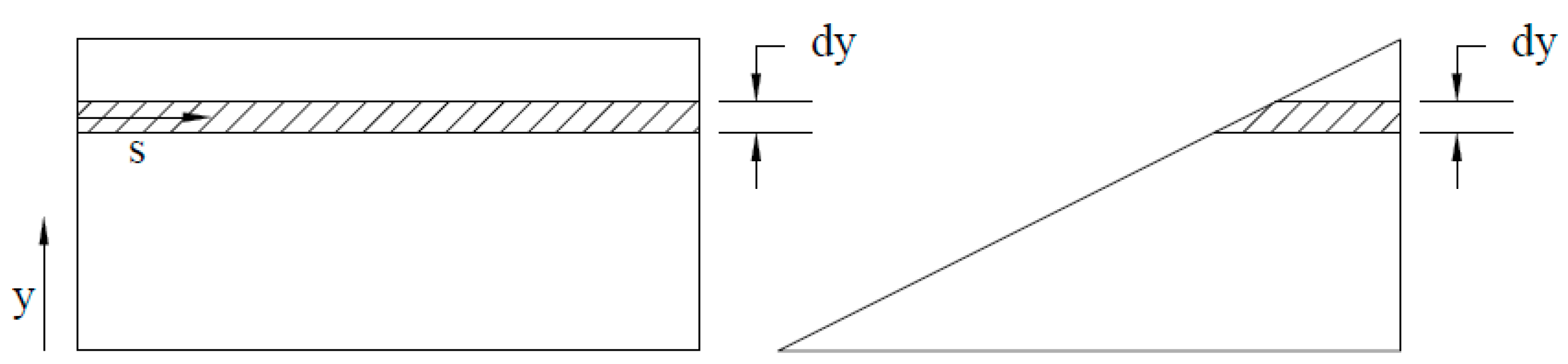
3. Estimating the Bound and Trailed Circulation from CFD

Even though the VG aspect ratio was low, it was still assumed that the flow was locally 2-D with only a small spanwise component and thereby the bound circulation at a given height could be estimated using the Kutta–Joukowski theorem from 2-D airfoil theory:

$$\mathrm{l}\left(\mathrm{y}\right)=\mathsf{\rho }{u}_{\mathrm{x}}\left(\mathrm{y}\right){\mathsf{\Gamma }}_{\mathrm{b}}\left(\mathrm{y}\right)$$

(1)

where y is the normal distance from the root of the VG, $\mathsf{\rho }$ is the fluid density, and Γ_b(y) is the bound circulation at each location. The bound circulation Γ_b(y), thus, varied with the VG geometry and the incoming flow as a function of the wall-normal distance y. The velocity profile shown in Figure 6 corresponds to the computed streamwise average velocity profile at 3h upstream i.e., x/h = −3h, where the flow was undisturbed by the vanes.

First, the pressure load normal to the VG surface [N/m] was found by integrating the pressure jump at the height y from the leading edge, s = 0, to trailing edge, s = c(y), of the VG, as shown in Figure 7.

$${\mathrm{f}}_{\mathrm{n}}\left(\mathrm{y}\right)={{\displaystyle \int }}_{s=0}^{\mathrm{s}=\mathrm{c}\left(\mathrm{y}\right)}\Delta \mathrm{p}\left(\mathrm{s},\mathrm{y}\right)\mathrm{ds}$$

(2)

Since the pressure force acted perpendicularly to the VG surface, the lift force was estimated by projecting this with the geometric pitch angle, β, of the VG to the incoming flow, as

$$\mathrm{l}\left(\mathrm{y}\right)={\mathrm{f}}_{\mathrm{n}}\left(\mathrm{y}\right)\cos \mathsf{\beta }$$

(3)

The trailed vortices from this distribution of local lift would change the inflow, so that the angle should more accurately also be corrected with the induction, for example, as described in [25] for the case of a wind turbine blade. A numerical test was made to estimate the influence of using the lift distribution calculated directly from Equation (3) on the inflow, which was then used as an angle when projecting the pressure force to find a more accurate lift distribution. It was concluded that the effect on the final bound circulation distribution was quite small when taking the cosine to the angle and, therefore, only the geometric angle was used when estimating the lift distribution from the pressure difference, across the vortex generator.

The bound circulation can now be computed from Equation (1), as

$${\mathsf{\Gamma }}_{\mathrm{b}}\left(\mathrm{y}\right)=\frac{\mathrm{l}\left(\mathrm{y}\right)}{{\mathsf{\rho }\mathrm{u}}_{\mathrm{x}}\left(\mathrm{y}\right)}$$

(4)

To fulfill Helmholtz’s theorem, vortex filaments with strength equal to the gradient of the bound circulation must be trailed from the trailing edge, as

$${\mathrm{d}\mathsf{\Gamma }}_{\mathrm{t}}=\mathsf{\gamma }\left(\mathrm{y}\right)\mathrm{dy}$$

(5)

where γ is the distribution of bound circulation. However, after some short downstream distance, these trailed vortices would curl up to one strong tip vortex with strength

$${\mathsf{\Gamma }}_{\mathrm{t}}={{\displaystyle \int }}_{{\mathrm{h}}_s}^{\mathrm{h}}\mathsf{\gamma }\left(\mathrm{y}\right)\mathrm{dy}={{\displaystyle \int }}_{{\mathrm{h}}_{\mathrm{s}}}^{\mathrm{h}}{\mathrm{d}\mathsf{\Gamma }}_{\mathrm{b}}\left(\mathrm{y}\right)$$

(6)

This was such that the strength of the trailed vortex simply became the integral of the bound circulation from the some starting value, h_s, to the tip y = h. If it had been a pure airplane wing, one should start the integration at y = 0, but to avoid interference with the horizontal wall at y = 0, the starting value was set to a fraction of the VG height and the value chosen was 0.2h. From quantitative estimation, one can observe that the circulation for the innermost part of the VG did not contribute significantly to the tip vortex. This can also be understood from the flow visualization presented in at the end of the results section. To estimate the strength of the tip vortex from the computed flow in the wake of the VGs, one could apply the best fit to a Lamb–Oseen Vortex (LOV) (in polar coordinates).

$${\mathrm{u}}_{\mathsf{\theta }}\left(\mathrm{r}\right)=\frac{{\mathsf{\Gamma }}_{\mathrm{LOV}}}{2\mathsf{\pi }\mathrm{r}}\left(1-\exp \left(-\frac{{\mathrm{r}}^2}{{\mathsf{\epsilon }}^2}\right)\right)$$

(7)

where ε is a parameter that characterizes the radius of the vortex. This approach was first implemented for vortex generators in [9] and later applied in the works of others, e.g., in [26]. An alternative approach is to estimate the strength of the VG generated vortex by the path integral of the velocity component in the tangential direction (in polar coordinates) as,

$${\mathsf{\Gamma }}_{\mathrm{t}}=\underset{0}{\overset{2\mathsf{\pi }}{{\displaystyle \int }}}{\mathrm{u}}_{\mathsf{\theta }}\mathrm{rd}\mathsf{\theta }$$

(8)

Two constraints are taken into account for choosing the most representative radius r. First, the radius should be large enough to enclose all vorticity from one vortex and small enough to not be influenced by the neighboring vortex. The hypothesis that the vortex strength can be estimated from the distribution of bound circulation on the VG, as in Equation (6), could now be tested by comparing it to the circulation behind the VG computed directly from the velocity in the vortex, using Equations (7) and (8). If this hypothesis was valid, then one could estimate the expected strength from the boundary profile, as the one shown in Figure 6, and by assuming some airfoil data Cl(α) for the profiles used on the VG (often simply a thin flat plate), where the angle of attack was approximately the pitch angle β.

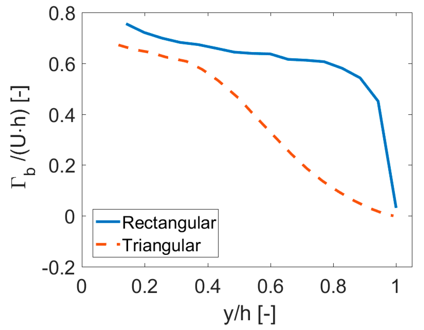
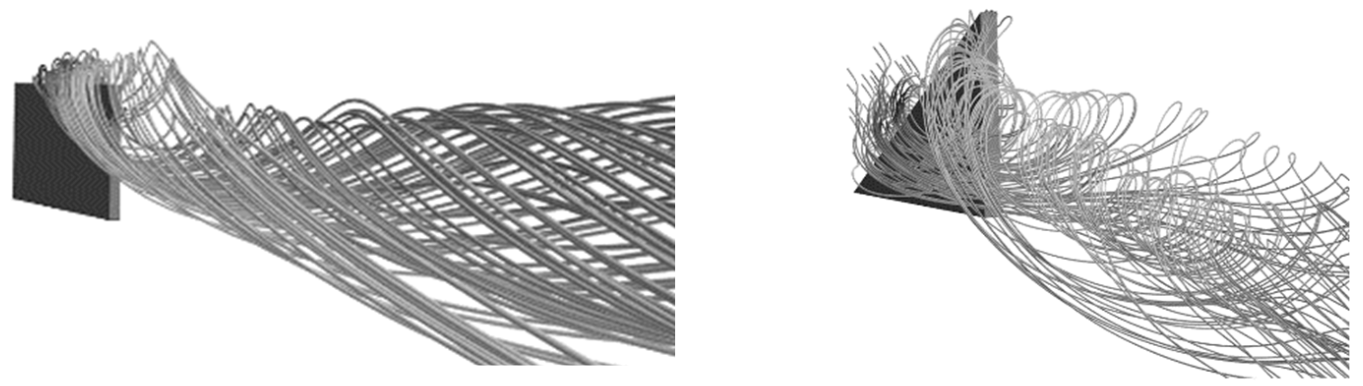
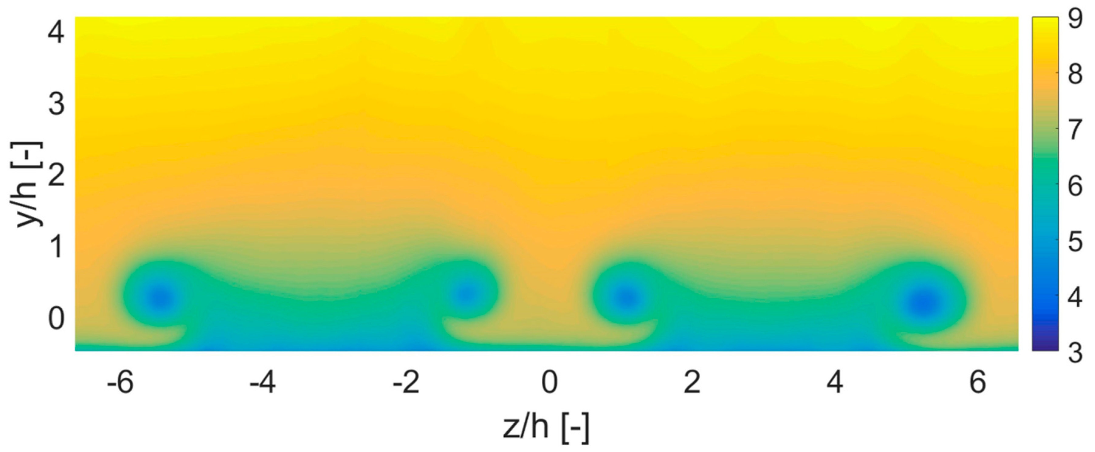
4. Results and Discussion

Figure 8 and Figure 9 display the obtained circulation in the wake found from Equations (7) and (8), for the rectangular and triangular VGs, respectively. Each subfigure of these two Figures compares the experimental results to the CFD results from one of the applied turbulence models, on the (left) Reynolds stress model, (middle) the k-ω SST, and (right) the Spalart–Allmaras model. The path integrated circulation obtained from the experiments (o) and from the simulations (x) was also compared to the LOV circulation estimate (+). The circulation was calculated in five and two downstream planes for the rectangular (Figure 8) and triangular (Figure 9) configurations, respectively.

The experimentally determined circulation was computed from the (ensemble) averaged measurements/simulations, so the meandering effects would impair the resulting circulation, as can be seen in the downstream development. The Reynolds Stress Turbulence (RST) model (Figure 8, left) provides the most satisfactory comparison between the experimental [20,21] and the numerical results, using the STAR CCM+ model herein.

For the triangular VG geometry, the circulation is investigated in two downstream planes, as shown in Figure 9, since the ensemble averaged vortex cores in this setting were not always well distinguishable beyond 12h after the VGs, due to meandering [20,21]. For the first downstream plane, the triangular geometry yielded a similar circulation, compared to the rectangular, while the RST turbulence model result was again the most accurate fit between the experimental and the numerical results. A better agreement was expected for the RST model since it includes correlations (flow history effects) and it is not based on an eddy viscosity model (e.g., the two-equation and other lower order models). Furthermore, RST models can better capture the large-scale vortex motion through the inclusion of the material derivative of the $\overline{u_i^{\prime }{u}_j^{\prime }}$ correlations and it does not impose local isotropy or eddy viscosity in the same manner as lower order models [27,28]. The lower order models are widely known to not be able to capture large scale gradients, including stagnation, separation, and rotation, which is in fact the hallmark of the flows produced by VGs.

As expected, the circulation estimated by the LOV was lower compared to the one estimated by the line integration, due to the inherent axi-symmetry of the LOV approach (see Figure 10).

Since the RST turbulence model provides the most accurate comparison between the experimental and numerical results for both geometries, it is used to validate the hypothesis for the estimation of the generated vortex strength from the spanwise distribution of bound circulation. This distribution along the VG height, obtained from the RST simulation, is depicted for both investigated geometries in Figure 11. As expected, the bound circulation weakens from the root to the tip of the VG height.

However, significant differences in bound circulation distribution of the two tested geometries can be observed. For the rectangular case (Figure 11, solid curve), the bound circulation displays an approximately flat distribution within a height range of y/h = [0.2:0.8], followed by a sharp drop due to the abrupt termination in VG geometry near the top. In the triangular VG case (Figure 11, dashed curve), the slope decreases approximately linearly across the main part of the VG, which is expected due to the linearly varying chord length with VG height. More careful inspection reveals an inflection point (the curvature changes sign) at approximately y/h ≈ 0.6. This behavior is clearer in the circulation of the trailed filaments, shown in Figure 12, which are estimated from the gradient of the bound circulation. Here, the effect is instead manifested in a shift in the slope of the trailed circulation at y/h ≈ 0.6.

For the rectangular VGs (Figure 12, left), the trailed circulation is strongest near the tip since the spanwise gradient is the highest. This indicates that the downstream vortex is mostly generated near the tip of the vane. For the triangular VGs (Figure 12, right), the highest magnitude of the trailed circulation is observed in the vicinity of the inflection point, while most of the vortex filaments contribute to the circulation of the downstream vortex in contrast to the rectangular ones. This can be explained by the fact that vorticity is accumulated along the entire inclined edge of the triangular vane in order to form the vortex into the wake, as can be seen in Figure 13.

The formation of the trailing vortex, thus, did not only occur near the tip, but in fact occurred throughout the collection of the released trailing vortex filaments along the entire edge, and rolled up to one strong vortex core, as seen in Figure 13 (right). This might also explain why the vortex cores formed behind triangular VGs are sometimes significantly more distorted from axi-symmetry than those generated from rectangular VGs (c.f. [9,24]). For the rectangular VGs, the summation of the circulation of the filaments between y = 0.2h and the tip resulted in a numerical value Γ_t/U∙h = 0.65, which was almost identical with the value obtained from the line integration and the LOV, see Figure 8. The trailed circulation for the triangular VG from the integration of the bound circulation was equal to Γ_t/U∙h = 0.61 and was still quite close to the value of 0.55 estimated from the wake flow using LOV and line integration, which further supported the hypothesis.

5. Conclusions

In the current investigations, PIV measurements and RANS simulations were used to verify the hypothesis that the strength of the streamwise vortex behind a VG, which is responsible for mixing the boundary layer, could be found from the distribution of bound circulation, which in an engineering model could be estimated from 2-D airfoil data, assuming local 2-D flow at different heights from the root of the VG. Such an approach has been suggested by Poole et al. [29], where they formally applied a classical lifting line model to model the strength of the generated vortex from several VG geometries, and compared this to the measurements by Wendt [30]. Depending on how the bound circulation was estimated from airfoil theory, the errors varied between 5% to 25%. In this paper, the bound circulation at various wall-normal distances along the VG was determined by CFD and not by airfoil data. From this distribution, the trailed vortices were determined in the same way as in a classical lifting line model and very good agreement with the values computed from the wake velocities was found. Additionally, the trailed circulation from the CFD fit well with the experimentally obtained trailed circulation and the trends were consistent for both the classical rectangular and triangular VG shapes. All of this supported the idea of making an engineering approach that can estimate the strength of the generated streamwise vortex, based on the upstream boundary layer profile and the VG geometry, where the spanwise bound circulation is then determined from some assumed 2-D airfoil data, for the various profiles used along the VGs.

By knowing the circulation distribution on the VG one can, therefore, expect to quite accurately estimate the strength of the trailed vortex. However, the purpose of this study was not to refine such a model but to verify that the assumptions behind this approach were valid. It could even be possible to implement higher order models of this kind, e.g., by considering time variations in the flow to improve the prediction accuracy. Additionally, the spanwise distribution of the bound circulation was, as expected, quite different when using a triangular shaped VG than that when using a rectangular VG in the same boundary layer, resulting in a different vortex structure, as seen in Figure 12 and Figure 13.

References

1. Taylor, H.D. The Elimination of Diffuser Separation by Vortex Generators; Research Department Report No. R-4012-3; United Aircraft Corporation: East Hartford, CT, USA, 1947. [Google Scholar]
2. Taylor, H.D. Design Criteria for and Applications of the Vortex Generator Mixing Principle; Research Department Report No. M-15038-1; United Aircraft Corporation: East Hartford, CT, USA, 1948. [Google Scholar]
3. Taylor, H.D. Summary Report on Vortex Generators; Research Department Report No. R-05280-9; United Aircraft Corporation: East Hartford, CT, USA, 1950. [Google Scholar]
4. Wang, H.; Zhang, B.; Qiu, Q.; Xu, X. Flow control on the NREL S809 wind turbine airfoil usingvortexgenerators. Energy 2017, 118, 1210–1221. [Google Scholar] [CrossRef]
5. Xia, H.H.; Tang, G.H.; Shi, Y.; Tao, W.Q. Simulation of heat transfer enhancement by longitudinalvortexgeneratorsin dimple heat exchangers. Energy 2014, 74, 27–36. [Google Scholar] [CrossRef]
6. Luo, L.; Du, W.; Wang, S.; Wang, L.; Zhang, X. Multi-objective optimization of a solar receiver considering both the dimple/protrusion depth and delta-wingletvortexgenerators. Energy 2017, 137, 1–19. [Google Scholar] [CrossRef]
7. Ma, T.; Pandit, J.; Ekkad, S.V.; Huxtable, S.T.; Wang, Q. Simulation of thermoelectric-hydraulic performance of a thermoelectric powergeneratorwith longitudinal vortexgenerators. Energy 2015, 84, 695–703. [Google Scholar] [CrossRef]
8. Ebrahimi, A.; Rikhtegar, F.; Sabaghan, A.; Roohi, E. Heat transfer and entropy generation in a microchannel with longitudinal vortex generators using nanofluids. Energy 2016, 101, 190–201. [Google Scholar] [CrossRef]
9. Velte, C.M.; Hansen, M.O.L.; Okulov, V.L. Helical structure of longitudinal vortices embedded in turbulent wall-bounded flow. J. Fluid Mech. 2009, 619, 167–177. [Google Scholar] [CrossRef] [Green Version]
10. Pearcey, H.H. Shock Induced Separation and Its Prevention by Design and Boundary Layer Control. In Boundary Layer and Flow Control; Lachmann, G.V., Ed.; Pergamon Press: Oxford, UK, 1961; Volume 2, pp. 1166–1344. [Google Scholar]
11. Jones, J.P. The Calculation of Paths of Vortices from a System of Vortex Generators, and a Comparison with Experiments; Aeronautical Research Council, Technical Report C.P. No. 361; Aeronautical Research Council: London, UK, 1957. [Google Scholar]
12. Smith, F.T. Theoretical prediction and design for vortex generators in turbulent boundary layers. J. Fluid Mech. 1994, 270, 91–131. [Google Scholar] [CrossRef]
13. Lamb, H. Hydrodynamics, 6th ed.; Cambridge University Press: Cambridge, UK, 1932. [Google Scholar]
14. Hansen, M.O.L.; Westergaard, C. Phenomenological Model of vortex generators. In IEA, Aerodynamics of Wind Turbines, 9th Symposium; IEA: Paris, France, 1995; pp. 1–7. [Google Scholar]
15. Chaviaropoulos, P.K.; Politis, E.S.; Nikolaou, I.G. Phenomenological modeling of vortex generators. In Proceedings of the EWEC 2003, Madrid, Spain, 16–19 June 2003. [Google Scholar]
16. Velte, C.M.; Hansen, M.O.L.; Okulov, V. Multiple vortex structures in the wake of a rectangular winglet in ground effect. Exp. Therm. Fluid Sci. 2016, 72, 31–39. [Google Scholar] [CrossRef] [Green Version]
17. Charalampous, A.; Foucaut, J.M.; Cuvier, C.; Velte, C.M.; Hansen, M.O.L. Verification of numerical modeling of VG flow by comparing to PIV data. In Proceedings of the Wind Energy Science Conference 2017, Kgs. Lyngby, Denmark, 26–29 June 2017. [Google Scholar]
18. Bender, E.E.; Anderson, B.H.; Yagle, P.J. Vortex generator modeling for Navier Stokes codes. In Proceedings of the 1999 3rd ASME, FEDSM’99-6929, San Francisco, CA, USA, 18–23 July 1999. [Google Scholar]
19. Manolesos, M.; Sørensen, N.N.; Troldborg, N.; Florentie, L.; Papadakis, G.; Voutsinas, S. Computing the flow past Vortex Generators: Comparison between RANS Simulations and Experiments. The Science of Making Torque from Wind (TORQUE 2016). IOP Publ. J. Phys. Conf. Ser. 2016, 753, 022014. [Google Scholar] [CrossRef]
20. Velte, C.M.; Braud, C.; Coudert, S.; Foucaut, J.-M. Vortex generator induced flow in a high re boundary layer. J. Phys. Conf. Ser. (Online) 2014, 555, 012102. [Google Scholar] [CrossRef]
21. Foucaut, J.M.; Coudert, S.; Braud, C.; Velte, C. Influence of light sheet separation on SPIV measurement in a large field spanwise plane. Measurement Sci. Technol. 2014, 25, 035304. [Google Scholar] [CrossRef]
22. STAR CCM + Users Manual. Available online: http://www.cd-adapco.com/products/star-ccm/documentation (accessed on 2 June 2019).
23. Fernández-Gámiz, U.; Velte, C.M.; Réthoré, P.E.; Sørensen, N.N.; Egusquiza, E. Testing of self-similarity and helical symmetry in vortex generator flow simulations. Wind Energy 2016, 19, 1043–1052. [Google Scholar] [CrossRef]
24. Velte, C.M.; Hansen, M.O.L.; Cavar, D. Flow analysis of vortex generators on wing sections by stereoscopic particle image velocimetry measurements. Environ. Res. Lett. 2008, 3, 015006. [Google Scholar] [CrossRef]
25. Rahimi, H.; Schepers, J.G.; Shen, W.Z.; Ramos Garcia, N.; Scneider, M.S.; Micallef, D.; Simao Ferreira, C.J.; Jost, E.; Klein, L.; Herráez, I. Evaluation of different methods for determining the angle of attack on wind turbine blades with CFD results under axial inflow conditions. Renew. Energy 2018, 125, 866–876. [Google Scholar] [CrossRef] [Green Version]
26. Martínez-Filgueira, P.; Fernandez-Gamiz, U.; Zulueta, E.; Errasti, I.; Fernandez-Gauna, B. Parametric study of low-profile vortex generators. Int. J. Hydrogen Energy 2017, 42, 17700–17712. [Google Scholar] [CrossRef]
27. Launder, B.; Reece, G.; Rodi, W. Progress in the development of a Reynolds-stress turbulence closure. J. Fluid Mech. 1975, 68, 537–566. [Google Scholar] [CrossRef] [Green Version]
28. Gibson, M.; Rodi, W. A Reynolds-stress closure model of turbulence applied to the calculation of a highly curved mixing layer. J. Fluid Mech. 1981, 103, 161–182. [Google Scholar] [CrossRef]
29. Poole, D.J.; Bevan, R.L.T.; Allen, C.B.; Rendall, T.C.S. An Aerodynamic Model for Vane-Type Vortex Generators. In Proceedings of the 8th AIAA Flow Control Conference, Washington, DC, USA, 13–17 June 2016. [Google Scholar]
30. Wendt, J. Parametric study of vortices shed from airfoil vortex generators. AIAA J. 2004, 42, 2185–2195. [Google Scholar] [CrossRef]
Figure 1. A sketch of the Laboratoire de Mécanique des Fluides de Lille (LMFL) wind tunnel (figure originally extracted from http://lml.univ-lille1.fr/?page=144&menu_curr_set=144).
Energies 12 02781 g001
Figure 2. Top-view of the configuration design showing the geometric parameters (top). A 3-D drawing of the set-up (bottom).
Energies 12 02781 g002
Figure 3. Schematic of the Stereoscopic Image Velocimetry setup.
Energies 12 02781 g003
Figure 4. Example of the ensemble averaged velocity field at 3h downstream of the rectangular vortex generators (VGs).
Energies 12 02781 g004
Figure 5. Prism layers attached to the rectangular VGs (top). Top-view of the mesh discretization of the rectangular VGs (bottom).
Energies 12 02781 g005
Figure 6. Streamwise average velocity profile at 3h upstream, Reynolds Stress Turbulence (RST) turbulence model.
Energies 12 02781 g006
Figure 7. Integrating the pressure jump at the height y from the leading edge s = 0 to the trailing edge s = c(y) for determining the load fn(y) [N/m] normal to the VGs surface.
Energies 12 02781 g007
Figure 8. Circulation results for the rectangular configuration testing Reynolds Stress, k-ω SST, Spalart–Allmaras turbulence models in five downstream planes; (left) Reynolds stress model, (middle) k-ω SST, and (right) Spalart–Allmaras.
Energies 12 02781 g008
Figure 9. Circulation results for the triangular configuration testing Reynolds Stress, k-ω SST, Spalart–Allmaras turbulence models in two downstream planes; (left) Reynolds stress model, (middle) k-ω SST, and (right) Spalart–Allmaras.
Energies 12 02781 g009
Figure 10. Determination of Γ with the use of Lamb–Oseen Vortex, (left) rectangular VG and (right) triangular VG, RST turbulence model.
Energies 12 02781 g010
Figure 11. Distribution of the bound circulation along VGs height.
Energies 12 02781 g011
Figure 12. Distribution of the trailed circulation along VGs height. Rectangular VG (left) and triangular VG (right).
Energies 12 02781 g012
Figure 13. Trailing vortex associated streamlines visualized for the (left) rectangular and (right) triangular vortex generators, RST turbulence model.
Energies 12 02781 g013