A Master/Slave Approach to Power Flow and Overvoltage Control in Low-Voltage Microgrids

Abstract

This paper proposes a technique to control distributed energy resources in low-voltage microgrids aiming at (i) allowing power flow control at the point of connection with the upstream grid, (ii) keeping voltage profiles within the operational limits. The first feature is crucial in smart low-voltage power systems. In fact, it enables both demand-responses, which is extremely valuable from the point of view of distribution system operators and for energy trading, and the autonomous operation of the microgrid. The latter can be achieved by regulating to zero the power exchanged with the main grid. The second feature allows to limit voltage increases due to active power injection by distributed energy resources and, thus, to limit stresses on the electrical infrastructure and the served loads, which is a concrete issue as renewables become widely deployed in the low-voltage scenario. The proposed approach is firstly described in detail, then a systematic analysis of its local and global properties is reported. All the obtained results are verified considering the IEEE 37 test feeder in realistic operating conditions.

1. Introduction

Low-voltage microgrids will play a major role in future power systems [1,2]. The deployment of distributed micro-generation and energy storage owned by end users results in a new paradigm for electrical grids and in a potentially new and exciting market for technology manufacturers, service providers, energy traders, distributors, and regulatory boards.

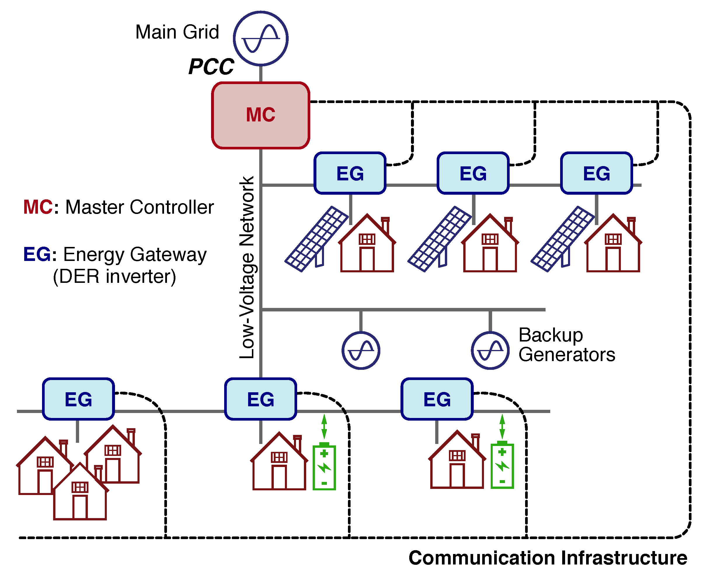
Smart microgrids are a portion of the low-voltage distribution network which feature a high penetration of distributed energy resources (DERs) and are able to operate both connected and disconnected from the main electricity grid [3]. In this scenario, customers are envisioned to be active agents that cooperate and participate to the operation of the microgrid, e.g., by coordinating their resources to receive economical benefits [4]. This is enabled by the power control flexibility given by electronic power converters, which interface DERs with the grid. The operation of such systems, herein referred to as energy gateways (EG), is typically supervised by a microgrid controller, herein referred to as master controller (MC) [5], forming structures of the kind represented in Figure 1.

A high penetration of DERs can cause intermittent energy production and power imbalance [6,7]. However, proper control schemes will guarantee reliable operation and efficient integration of green technologies by means of electronic converters in low-voltage distribution grids [8,9].

In recent years there has been a growing interest in methods for the control and optimization of the resources of microgrids. Significant research efforts have been devoted to the solution of the optimal power flow problem considering various functional costs (e.g., power losses, voltage deviations) and physical constraints of the electrical network. In general, the proposed algorithms can be divided into four classes:

• decentralized, algorithms that are purely local, without any communication among agents;
• distributed: algorithms where each agent communicates with its neighbors (typically the physically closest agents), but a centralized unit or controller is not present;
• hierarchical: algorithms where the control is performed by agents that communicate with entities at the higher level of a hierarchical structure, in which a centralized controller implements the top level;
• centralized: where agents directly communicate with a centralized controller that performs computations and coordinate the agents by sending proper control commands.

A comprehensive survey on multi-agent methodologies applied to smart power systems scenarios is provided, for example, in [10,11,12,13]. It is worth stressing that most of the multi-agent strategies proposed in the literature can be classified as model-based, namely, it is assumed that a model of the grid is available, including full knowledge of the network parameters, like lines’ impedance and network topology.

In this paper we address two main issues of low-voltage microgrids:

• regulation the power flow at the point of common coupling (PCC) between the microgrid and the main grid;
• the fulfillment of voltage constraints at grid nodes.

From the system operator point of view, controlling the microgrid power absorption, that is, the microgrid dispatchability, is fundamental. In the control scheme we propose, dispatchability is obtained by coordinating customer renewables availability. A microgrid central controller gathers from DERs information encoding their flexibility in accepting some directives on the required power injection, as envisioned by relevant standards and research papers (e.g., [5,14,15]), to attain a proper load sharing among agents and to control the power exchange at the point of common coupling (PCC). The aforementioned two goals usually relate to the primary and tertiary control level of traditional control hierarchies, respectively [16,17,18,19].

The violation of voltage constraints constitutes an unwanted operating condition to be tackled to preserve the quality of service. Furthermore, uniform voltage profiles along the the distribution lines is favorable in terms of network reliability and efficiency [20]. Voltage regularization is achieved herein by supporting the centralized scheme with a local dynamic overvoltage control. In this way, both the voltage regulation and the power exchange with the external distribution network are achieved. The overall master/slave architecture controls the operation of DERs in a centralized manner, while local regulators embedded in DERs intervene in case of overvoltage events. Local regulators limit the amount of injected power to keep the voltage at the output of the distributed converters limited below the upper allowed limit.

The control objectives are achieved on the basis of power measurements at the point of connection with the main grid and the power availability information from distributed energy resources. Notably, the approach is model-free, because it does not rely on any specific model of the distribution network or the distributed energy resources that are controlled. This control feature is valuable especially within the considered low-voltage application scenario, where network structure and parameters are often unknown and possibly changing.

The control scheme proposed herein was firstly introduced in [21], where it is referred to as power-based control. With respect to [21], this paper presents original aspects and additional analyses that mainly consist in a different local voltage-control rule, a formal and detailed description of the underlying algorithm, the stability analysis of both the local and global properties of the algorithm.

The remaining part of the paper is organized as follows. Section 2 introduces the considered microgrid architecture. Section 3 provides and describes in detail a model-free power-based control strategy of DERs. The stability analysis is provided in Section 4. Finally, numerical results in a realistic simulation scenario are reported in Section 5. Section 6 concludes the paper.

Notation

Lower- (upper-) case boldface letters denote column vectors (matrices). Calligraphic symbols are reserved for sets. Symbol ${}^{\top }$ stands for transposition. Vectors $\mathbf{1}$ and ${\mathbf{e}}_m$ denote the all-one vectors and the m-th canonical vector, respectively. Given a set $\mathcal{A}$, $\left|\mathcal{A}\right|$ will denote the number of elements in $\mathcal{A}$.

2. Cyber-Physical Model of a Smart Microgrid Architecture

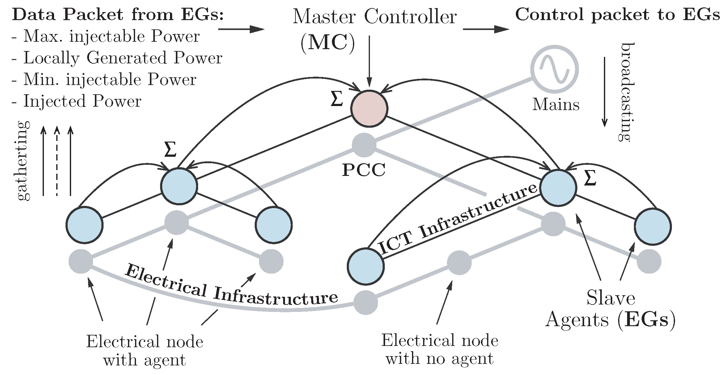
In this paper, we envision a microgrid as a cyber-physical system, as illustrated in Figure 2. The physical layer consists of the electrical infrastructure comprising the main grid, the distributed energy resources, and the electrical distribution network. The cybernetic layer represents the information and communication technology (ICT) infrastructure needed for the control and the monitoring of the electrical layer, and includes the sensors, the computation units, and the communication links and modules.

2.1. Electrical Physical Layer

To conveniently model the electrical physical layer we introduce a directed weighted graph $\mathcal{G}=\left(\mathcal{V},\mathcal{E}\right)$ where nodes in $\mathcal{V}$ correspond to buses, and edges $\mathcal{E}$ to distribution lines. Let $z_e=r_e+j{x}_e$ be the impedance of line e, where $r_e$ and $x_e$ are, respectively, the resistive and the inductive components. Because low-voltage grids are considered herein, we assume $r_e/x_e>>1$ for each $e\in \mathcal{E}$, namely, that the interconnection lines are mainly resistive, which is typical in low-voltage grids.

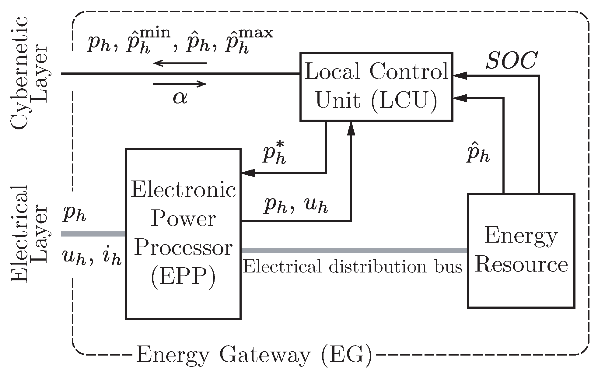
In our setup, buses can be either DERs or loads. A DER that can be controlled is referred to as an EG. Figure 3 depicts the structure of an EG. The energy source of an EG can be a combination of renewable sources and storage devices. Furthermore, an EG is equipped with a local control unit (LCU) and an electronic power processor (EPP), which interfaces the energy resources with the grid. The EG interacts with the electrical layer through the EPP, and with the cybernetic layer through the LCU. The LCU generates the set-point of power to be injected into the grid by the EPP. Figure 3 introduces a set of parameters (e.g., ${\widehat{p}}_k$, $\alpha$) that are related to the state of the EG or of the microgrid; these parameters are detailed in Section 3.

In our setup, the microgrid is fed by an ideal voltage source at the PCC, considered as the slack node of the microgrid. Formally, the electrical physical layer is described by the following variables:

• $\mathbf{u}\in {\mathbb{C}}^n$, where n is the total number of nodes (i.e., $\left|\mathcal{V}\right|=n$) and where the k-th component of $\mathbf{u}$ (i.e., $u_k$) is the grid complex voltage at node k;
• $\mathbf{i}\in {\mathbb{C}}^n$, where $i_k$ is the current injected at node k;
• $\mathbf{s}=\mathbf{p}+j\mathbf{q}\in {\mathbb{C}}^n$, where $s_k$, $p_k$, and $q_k$ are the nodal complex, active, and reactive power at node k, respectively.
• $\mathbf{v}\in {\mathbb{R}}^n$, where $v_k$ represents the voltage magnitude at node k.

By labeling with the subscript 0 the quantities associated with the PCC, the system variables satisfy the following equations:

$$\begin{array}{c}\mathbf{i}=\mathbf{Y}\mathbf{u}\hfill \end{array}$$

(1a)

$$\begin{array}{c}{u}_0=U_N\hfill \end{array}$$

(1b)

$$\begin{array}{c}{u}_k{\overline{i}}_k=p_k+i{q}_{k}h\ne 0\hfill \end{array}$$

(1c)

where $\mathbf{Y}$ is the bus admittance matrix and $U_N$ is the nominal grid voltage. It can be shown that there exists a unique matrix $\mathbf{Z}\in {\mathbb{C}}^{n\times n}$, called the Green matrix, that allow us to write voltages as a function of currents via:

$$\mathbf{u}=\mathbf{Z}\mathbf{i}+\mathbf{1}{U}_N.$$

(2)

Notably, the Green matrix is symmetric and positive semidefinite (see [22]). In the scenario we consider, where the distribution lines are mainly resistive [23], the non-linear relation between power injections and voltage magnitudes can be approximated with the linear function

$$\mathbf{v}\approx \frac{1}{U_N}\mathbf{R}\mathbf{p}+\mathbf{1}{U}_N$$

(3)

where the matrix $\mathbf{R}$ is the real part of $\mathbf{Z}$, i.e., $\mathbf{R}=\mathrm{real}\left(\mathbf{Z}\right)$. Numerical tests report voltage magnitude approximation errors less than 0.005 pu; see [24]. Equation (3) models the fact that, in mainly resistive networks, voltage amplitudes are determined by active power injections at the nodes of the grid [23].

2.2. Cyber Layer

In this paper, a master/slave controller aiming at supervising the operation of a microgrid is devised. The master controller (MC) is assumed to be located at the PCC of the microgrid and the EGs, which are geographically distributed, play as slave units. Both the MC and the EGs present some computational and sensing capabilities [25,26], e.g., they can take power and voltage measurements at their point of connection within the electrical network. Furthermore, the master unit (i.e., the MC) is assumed to be able to communicate with the slave units (i.e., the EGs) via a communication channel. (An investigation about the feasibility of such approaches in terms of communication requirements is presented in [27], referring to, in particular, the Long-Term Evolution (LTE) technology.)

3. A Model-Free Power-Based Control Strategy

This section presents an algorithm aiming at regulating the power injection of the EGs so that (i) the power flow at the microgrid’s PCC (i.e., the PCC power flow) follows a pre-assigned profile, denoted, in the following as $p_0^{*}$, (ii) the voltage magnitudes at the point of connection of the EGs are below a given threshold $U_{max}$. Reactive power control is not considered herein, but a similar approach may be employed to this purpose too, as outlined in [21].

The PCC power flow regulation is performed in two phases. In the first, the MC collects from each EG a data packet conveying information about its local energy availability; in the second, the MC broadcasts to all the EGs a common control packet which will be finally translated into power references. (It is worth highlighting that to broadcast a unique packet to all the controllable units is an advantageous feature of the approach, because it allows to limit the amount of data exchange through the communication infrastructure.) Figure 2 shows pictorially the control algorithm steps. In particular circumstances, due to the power injection by distributed energy resources, overvoltage conditions may appear at some nodes of the grid. Such nodes experiencing overvoltage are referred to as critical nodes.In the devised algorithm, EGs connected to critical nodes control active power injections by applying a purely local rule that limits the power injection to keep the voltage magnitude below the threshold $U_{max}$. This mode of operation is cleared by the MC when specific conditions at PCC are met, as described later on. To account for this, the algorithm formulation makes use of the set ${\mathcal{H}}_{\ell }$, which collects the EGs connected to critical nodes during the ℓ-th control cycle.

The algorithm is explained in details in the following.

3.1. Gathering of the Status of EGs

Assume that EGs regulate their output power injection every T seconds and refer to the time interval $\left](\ell -1)T,\ell T\right]$ as the ℓ-th control cycle. For $k\in \left\{1,\dots ,m\right\}$, where m denotes the number of EGs in the microgrid and EG${}_k$ is the k-th EG, EG${}_k$ communicates to the MC the following packet of data at the end of the $(\ell -1)$-th cycle:

• the active power $p_k\left[(\ell -1)T\right]$ injected at time instant $(\ell -1)T$ [for convenience quantities are denoted hereafter by indicating only the relevant control cycle, i.e., by using $p_k\left(\ell \right)$ instead of $p_k\left(\ell T\right)$];
• an estimate of the active power that will be generated by the local renewable source during the next control cycle, denoted as ${\widehat{p}}_k\left(\ell \right)$;
• the estimated minimum active power ${\widehat{p}}_k^{min}\left(\ell \right)$ and maximum active power ${\widehat{p}}_k^{max}\left(\ell \right)$ that may be injected during the next control cycle. The quantities ${\widehat{p}}_k^{min}\left(\ell \right)$ and ${\widehat{p}}_k^{max}\left(\ell \right)$ are computed by taking into account the maximum power that can be absorbed (${\widehat{p}}_{Sh}^{\mathrm{in}}$) or injected (${\widehat{p}}_{Sh}^{\mathrm{out}}$) by the local energy storage unit:

  $$\left\{\begin{array}{c}{\widehat{p}}_k^{min}\left(\ell \right)={\widehat{p}}_k\left(\ell \right)-{\widehat{p}}_{Sh}^{\mathrm{in}}\left(\ell \right)\hfill \\ {\widehat{p}}_k^{max}\left(\ell \right)={\widehat{p}}_k\left(\ell \right)+{\widehat{p}}_{Sh}^{\mathrm{out}}\left(\ell \right)\hfill \end{array}\right.$$

  (4)
• the overvoltage flag $h_k$, indicating whether the EG is a critical or non-critical node:

  $$h_k(\ell -1)=\left\{\begin{array}{cc}1& \mathrm{if}k\in {\mathcal{H}}_{\ell -1}\hfill \\ 0& \mathrm{if}k\notin {\mathcal{H}}_{\ell -1}\hfill \end{array}\right.$$

  (5)

The variables $p_k(\ell -1)$, ${\widehat{p}}_k\left(\ell \right)$, ${\widehat{p}}_k^{min}\left(\ell \right)$, ${\widehat{p}}_k^{max}\left(\ell \right)$, $h_k(\ell -1)$ represent the state of EG${}_k$ at the end of the $(\ell -1)$-th cycle.

3.2. Computation of the Microgrid State

Concurrently with the EGs operation, the MC measures the PCC power absorption $p_0(\ell -1)$ and receives from the EGs their data packets. Based on the collected information, the MC computes sequentially the following overall quantities for the entire grid:

• the total power provided by the EGs (i.e., the micro-generators):

  $$p_{tot}(\ell -1)=\sum _k{p}_k(\ell -1)$$

  (6)
• the total net load of the microgrid:

  $$p_L(\ell -1)=p_0(\ell -1)+p_{tot}(\ell -1)$$

  (7)

  which amounts at the sum of the overall electrical load power and the power loss along the distribution lines;
• the estimate of the total power that should be injected by the micro-generators in the next cycle:

  $$p_{tot}^{*}\left(\ell \right)=p_L(\ell -1)-p_0^{*}\left(\ell \right)$$

  (8)

  where $p_0^{*}$ is a pre-assigned power profile at the PCC of the microgrid. (From a practical standpoint, $p_0$ is negotiated with the distribution system operator and set to obtain the higher economic benefit for the microgrid; a choice that is technically convenient is, for example, to set $p_0^{*}$ constant and equal to the expected mean power absorption at the microgrid PCC.)

Based on the above quantities and on the states of the EGs, the MC assesses the overall power generation capability of the grid computing the three quantities ${\widehat{p}}_{tot}\left(\ell \right)$, ${\widehat{p}}_{tot}^{min}\left(\ell \right)$, ${\widehat{p}}_{tot}^{max}\left(\ell \right)$, which is the estimated total power the EGs can generate, the estimated total minimum and maximum power the EGs can inject during the next control cycle, respectively. In particular, the MC distinguishes among two situations, that is, whether $p_{tot}(\ell -1)<p_{tot}^{*}\left(\ell \right)$ or $p_{tot}(\ell -1)>p_{tot}^{*}\left(\ell \right)$.

When it holds

$$p_{tot}(\ell -1)<p_{tot}^{*}\left(\ell \right)$$

(9)

the MC will commit an increment of micro-generators power injection in the next control cycle to fulfill power requests from the external grid. This is a critical condition, since increasing the power injections naturally brings to a further increase of bus voltages. As a consequence, the number of nodes experiencing overvoltage may rise, i.e., $\#{\mathcal{H}}_{\ell }\ge \#{\mathcal{H}}_{\ell -1}$. Hence, nodes that are critical should maintain their status (i.e., $h_k=1$) and avoid any increase of active power injection:

$${\widehat{p}}_k\left(\ell \right)={\widehat{p}}_k^{min}\left(\ell \right)={\widehat{p}}_k^{max}\left(\ell \right)=p_k(\ell -1).$$

(10)

Consequently,

$$\begin{array}{c}{\widehat{p}}_{tot}\left(\ell \right)=\sum _{k\notin {\mathcal{H}}_{\ell -1}}{\widehat{p}}_k\left(\ell \right)+\sum _{k\in {\mathcal{H}}_{\ell -1}}{p}_k(\ell -1)\hfill \\ {\widehat{p}}_{tot}^{min}\left(\ell \right)=\sum _{k\notin {\mathcal{H}}_{\ell -1}}{\widehat{p}}_k^{min}\left(\ell \right)+\sum _{k\in {\mathcal{H}}_{\ell -1}}{p}_k(\ell -1)\hfill \\ {\widehat{p}}_{tot}^{max}\left(\ell \right)=\sum _{k\notin {\mathcal{H}}_{\ell -1}}{\widehat{p}}_k^{max}\left(\ell \right)+\sum _{k\in {\mathcal{H}}_{\ell -1}}{p}_k(\ell -1)\hfill \end{array}$$

(11)

Instead, when the grid is in a non-critical condition, i.e.,

$$p_{tot}(\ell -1)\ge p_{tot}^{*}\left(\ell \right)$$

(12)

also the critical EGs can be exploited to their full potential in order to fulfill the external grid’s request. In this case:

$$\begin{array}{c}{\widehat{p}}_{tot}\left(\ell \right)=\sum _k{\widehat{p}}_k\left(\ell \right)\hfill \\ {\widehat{p}}_{tot}^{min}\left(\ell \right)=\sum _k{\widehat{p}}_k^{min}\left(\ell \right)\hfill \\ {\widehat{p}}_{tot}^{max}\left(\ell \right)=\sum _k{\widehat{p}}_k^{max}\left(\ell \right)\hfill \end{array}$$

(13)

Equations (11) and (13) can be grouped into a unique set of equations by making use of an auxiliary variable $\gamma$ that is set equal to 0 if $p_{tot}(\ell -1)>p_{tot}^{*}\left(\ell \right)$, 1 otherwise. In this way, (11) and (13) can be written compactly as:

$$\begin{array}{c}{\widehat{p}}_{tot}\left(\ell \right)=\sum _k\left(1-\gamma h_k\left(\ell \right)\right){\widehat{p}}_k\left(\ell \right)+\sum _k\gamma h_k(\ell -1)p_k(\ell -1)\hfill \\ {\widehat{p}}_{tot}^{min}\left(\ell \right)=\sum _k\left(1-\gamma h_k\left(\ell \right)\right){\widehat{p}}_k^{min}\left(\ell \right)+\sum _k\gamma h_k(\ell -1)p_k(\ell -1)\hfill \\ {\widehat{p}}_{tot}^{max}\left(\ell \right)=\sum _k\left(1-\gamma h_k\left(\ell \right)\right){\widehat{p}}_k^{max}\left(\ell \right)+\sum _k\gamma h_k(\ell -1)p_k(\ell -1)\hfill \end{array}$$

(14)

Observe that in (4), ${\widehat{p}}_k^{min}$ and ${\widehat{p}}_k^{max}$ are calculated assuming that all the power available from the renewable source [i.e., ${\widehat{p}}_k\left(\ell \right)$] is fully used, either by means of power injection into the grid or by charging local storage devices. The rationale behind (14) will become clear later on, while describing the algorithm proposed to control the microgrid.

3.3. Computation of the Control Command to Be Broadcasted

Based on the aforementioned quantities, the MC computes and broadcasts to all the EGs a control coefficient, denoted as $\alpha$. The value of the coefficient $\alpha$ depends both on the required power at the PCC and on the available power from EGs. To be specific, the coefficient $\alpha$ is computed as follows.

(i)

If $p_{tot}^{*}\left(\ell \right)<p_{tot}^{min}\left(\ell \right)$ then:

$$\alpha =0.$$

(15)

In this case, the loads are expected to absorb a total active power lower than the minimum power the active nodes can deliver. The overproduction is exported to the main grid.

(ii)

If $p_{tot}^{min}\left(\ell \right)\le p_{tot}^{*}\left(\ell \right)<{\widehat{p}}_{tot}\left(\ell \right)$ then:

$$\alpha ={\displaystyle \frac{p_{tot}^{*}\left(\ell \right)-{\widehat{p}}_{tot}^{min}\left(\ell \right)}{{\widehat{p}}_{tot}\left(\ell \right)-{\widehat{p}}_{tot}^{min}\left(\ell \right)}}.$$

(16)

In this case, the generated power is greater than the expected load. The generation excess can be accumulated into distributed storage units.

(iii)

If ${\widehat{p}}_{tot}\left(\ell \right)\le p_{tot}^{*}\left(\ell \right)\le p_{tot}^{max}\left(\ell \right)$ then:

$$\alpha =1+{\displaystyle \frac{p_{tot}^{*}\left(\ell \right)-{\widehat{p}}_{tot}\left(\ell \right)}{{\widehat{p}}_{tot}^{max}\left(\ell \right)-{\widehat{p}}_{tot}\left(\ell \right)}}.$$

(17)

In this case the expected load power is higher than the generated power but the difference can be supplied by distributed energy storage.

(iv)

If $p_{tot}^{*}\left(\ell \right)>p_{tot}^{max}\left(\ell \right)$ then:

$$\alpha =2.$$

(18)

In this case, the loads are expected to absorb a total power greater than the maximum power the active nodes can deliver. The power deficiency will be imported from the upstream grid.

In addition to $\alpha$, the MC broadcasts to the EGs also the value of $\gamma$, which is used by the EGs to update the flag variables as

$$h_k\left(\ell \right)=\gamma h_k(\ell -1),k\in \left\{1,\dots ,m\right\}.$$

3.4. Actuation by EGs of the Broadcasted Command

Once a new coefficient $\alpha$ is available, for $k\in \left\{1,\dots ,m\right\}$, EG${}_k$ determines its power injection as:

$$\begin{array}{cc}\hfill p_k^{*}=(1-& h_k\left(\ell \right)\left)\right(p_k^{min}\left(\ell \right)+\left({\widehat{p}}_k\left(\ell \right)-p_k^{min}\left(\ell \right)\right)min\left(\alpha ,1\right)+\hfill \\ & \left(p_k^{max}\left(\ell \right)-{\widehat{p}}_k\left(\ell \right)\right)·max\left(\alpha -1,0\right))+h_k\left(\ell \right)p_k(\ell -1)\hfill \end{array}$$

(19)

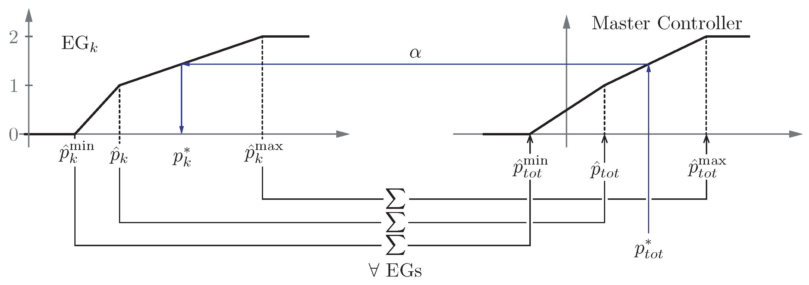
If EG${}_k$ is a critical node at the end of the $(\ell -1)$-th cycle and the MC does not clear its condition at the beginning of the ℓ-th cycle, then EG${}_k$ ignores the command from the MC and sets $p_k^{*}=p_k(\ell -1)$. Otherwise $p_k^{*}$ follows the profiles depicted in Figure 4 and, more explicitly, (19) can be rewritten in the four scenarios above identified as

(i)

if $p_{tot}^{*}\left(\ell \right)<p_{tot}^{min}\left(\ell \right)$ then

$$p_k^{*}=p_k^{min}\left(\ell \right).$$

(ii)

if $p_{tot}^{min}\left(\ell \right)\le p_{tot}^{*}\left(\ell \right)<{\widehat{p}}_{tot}\left(\ell \right)$ then

$$p_k^{*}=p_k^{min}\left(\ell \right)+{\displaystyle \frac{p_{tot}^{*}\left(\ell \right)-{\widehat{p}}_{tot}^{min}\left(\ell \right)}{{\widehat{p}}_{tot}\left(\ell \right)-{\widehat{p}}_{tot}^{min}\left(\ell \right)}}\left({\widehat{p}}_k\left(\ell \right)-p_k^{min}\left(\ell \right)\right).$$

Notice that in this case $p_k^{min}\left(\ell \right)\le p_k^{*}<{\widehat{p}}_k\left(\ell \right)$.

(iii)

if ${\widehat{p}}_{tot}\left(\ell \right)\le p_{tot}^{*}\left(\ell \right)\le p_{tot}^{max}\left(\ell \right)$ then

$${\widehat{p}}_k\left(\ell \right)+{\displaystyle \frac{p_{tot}^{*}\left(\ell \right)-{\widehat{p}}_{tot}\left(\ell \right)}{{\widehat{p}}_{tot}^{max}\left(\ell \right)-{\widehat{p}}_{tot}\left(\ell \right)}}\left(p_k^{max}\left(\ell \right)-{\widehat{p}}_k\left(\ell \right)\right).$$

Notice that in this case ${\widehat{p}}_k\left(\ell \right)<p_k^{*}<p_k^{max}\left(\ell \right)$.

(iv)

if $p_{tot}^{*}\left(\ell \right)>p_{tot}^{max}\left(\ell \right)$ then

$$p_k^{*}=p_k^{max}.$$

The principle of (19) is to make EGs participating to the microgrid power needs, measured at the PCC of the microgrid, in proportion to their capability of delivering or absorbing power, thus allowing a uniform exploitation of the resources available, without impeding EGs to pursue local objectives. Furthermore, heed that (19) makes use of the actual minimum and maximum injectable power values $p_k^{min},p_k^{max}$, which may differ from the estimated ${\widehat{p}}_k^{min},{\widehat{p}}_k^{max}$.

Assuming that all the data processing and communication amounts to a negligible fraction of the control period T, EG${}_k$ injects the power $p_k^{*}$ at time $\ell T^{+}$, that is, immediately after instant $\ell T$:

$$p_k\left(\ell T^{+}\right)=p_k^{*}.$$

(20)

3.5. $E{G}_k$ Local Control Rule

Recall that one of the objectives of the proposed algorithm is to keep the voltage amplitudes at the point of connection of the EGs below a specified threshold $U_{max}$. To do so, at the beginning of the $\ell -1$-th cycle, each EG${}_k$ measures $v_k$. If EG${}_k$ is experiencing an overvoltage, (An overvoltage can be due to different reasons, like, for example, increase of production from renewable sources, disconnection of large loads, connection of new generators, voltage magnitude adjustments by the distribution system operator.) it sets its flag variable $h_k$ equal to one (i.e., EG${}_k$ becomes a critical node) and adjusts the power injection according to the following rule:

$${\dot{p}}_k\left(t\right)=\phi (U_{max}-v_k\left(t\right))$$

(21)

where $\phi$ is a suitable positive constant, aiming at making its own voltage magnitude exactly equal to $U_{max}$. At the beginning of the ℓ-th control cycle, EG${}_k$ measures $v_k$ again. If EG${}_k$ is still having an overvoltage, it applies the local rule (21); otherwise, it keeps injecting the last power setpoint obtained from (21) in the $\ell -1$-th control cycle. EG${}_k$ applies the former procedure until its critical condition is reset by the MC, namely, when the signal $\gamma =0$ is sent; this is the reason why, as highlighted previously, if a node remains critical in the transition from the $(\ell -1)$-th to the ℓ cycle then it ignores the command $\alpha$.

The rationale behind this principle is that if EG${}_k$ is experiencing an overvoltage, i.e., $k\in {\mathcal{H}}_{\ell }$, then node k cannot absorb more power. Otherwise, the overvoltage condition would be worsened. Accordingly, by (21), EG${}_k$ starts to decrease $p_k$, counteracting the overvoltage condition. Of course, this relies on the assumption of operating on distribution grids that have a significant resistive component, which is typical in low-voltage microgrids.

Observe also that, if there exists $\tilde{t}$ such that $v_k\left(\tilde{t}\right)=U_{max}$, then the power $p_k\left(\tilde{t}\right)$ represents the power that the node where EG${}_k$ is connected can receive without experiencing overvoltages. In general, it might occur that, during the overvoltage condition, ${\widehat{p}}_k\left((\ell +1)T\right)<{\widehat{p}}_k^{min}(\ell +1)$; in this case the overproduction ${\widehat{p}}_k^{min}(\ell +1)-{\widehat{p}}_k\left((\ell +1)T\right)$ is assumed to be cut down (i.e., curtailed).

In Algorithm 1 a compact algorithmic description of the proposed control is reported. A representative illustration is displayed in Figure 4.

Algorithm 1 The following actions take place in the ℓ-th control cycle.

Consider the ℓ-th cycle. The following actions take place in the ℓ-th control cycle: Each EG${}_k$ sends $p_k(\ell -1)$, ${\widehat{p}}_k\left(\ell \right)$, ${\widehat{p}}_k^{min}\left(\ell \right)$, ${\widehat{p}}_k^{max}\left(\ell \right)$ and $h_k(\ell -1)$. On the basis of the received data, MC calculates quantities $p_{tot}(\ell -1)$, $p_L(\ell -1)$ and $p_{tot}^{*}\left(\ell \right)$ as in (6)–(8), respectively; If the grid is a critical situation (resp. not critical situation), MC computes computes ${\widehat{p}}_{tot}\left(\ell \right)$, ${\widehat{p}}_{tot}^{min}\left(\ell \right)$, ${\widehat{p}}_{tot}^{max}\left(\ell \right)$ as in (11) (resp. (13)); The MC computes (see (15)–(18)), and broadcasts to all the EGs the new value of $\alpha$; Each EG computes —by using (19)—and actuates its power reference $p_k^{*}$. For the full duration of the cycle, if EG${}_k$$\in {\mathcal{H}}_{\ell }$ and $v_k\left(\ell \right)\ge U_{max}$, EG${}_k$ keeps on applying the local control rule (21), otherwise $p_k\left(\ell \right)=p_k\left(\ell T\right)$.

Some relevant remarks are now reported in order.

Remark 1.

Both the MC and the EGs do not have any knowledge about the network’s model, meaning that the algorithm is model free.

Remark 2.

While the quantity $p_k$ can be measured directly, the quantities ${\widehat{p}}_k$, ${\widehat{p}}_k^{max}$, and ${\widehat{p}}_k^{min}$ have to be estimated locally. The estimation of ${\widehat{p}}_k$ can be done by considering the status of the installed renewable source (e.g., irradiation measurements for photovoltaic modules). On the other hand, the estimate of ${\widehat{p}}_k^{max}$ and ${\widehat{p}}_k^{min}$ can be done by considering the state of charge (SOC) of the local storage device, as indicated in (4), or to accommodate particular needs of the EG, by employing predictive models and statistical information.

Remark 3.

The EPPs are assumed to behave as current sources, conforming to current grid connection standards [28], as it is often the case in practical cases. Nevertheless, the proposed architecture and the made considerations keep valid also if EPPs behave as voltage sources (e.g., droop-like control [29]).

Remark 4.

The use of reactive power injections from the distributed converters to alter the voltage profiles has been shown to be an effective solution in medium-voltage (MV) networks [30,31,32], where interconnection cable impedances show significant inductive components (i.e., $r/x$ ratios are typically low). However, this approach is not suitable for low-voltage networks, where, interconnection impedances are mainly resistive (i.e., $r/x$ ratios are high) instead [33,34]. In fact, in networks with high $r/x$ ratios, the reactive power exchange needed to counteract voltage rises due to excessive active power injections might be so intense to bring additional detrimental effects on the electrical infrastructure (e.g., overload of MV/LV transformer and distribution cables) and also affect the reliability of the EPPs [35]. For this reason, approaches based on active power control are more effective in high $r/x$ microgrids, with the main drawback of a potential power production reduction, which, however, can be attenuated or even eliminated by small local accumulation.

Remark 5.

An advantage provided by distributed generation is that active power is generated close to the loads, which naturally limits voltage drops along distribution lines [20]. In addition, the control proposed herein adaptively coordinates the EGs power injection to be fairly shared among the generators (specifically, according to their power availability) and to match the microgrid power needs. This contributes to avoid undervoltage conditions. On the other hand, overvoltages are intrinsic issues of distributed generation in low-voltage grids. Overvoltages happen during periods of peak generation from renewables and may be favored by excessive power injections by the EGs (e.g., in response to remote control signals, like the those herein referred to as α). Notably, the proposed local overvoltage control technique deals with these particular issues.

4. Analysis of the Proposed Algorithm

In this section, Algorithm I is considered and analyzed in terms of:

• local properties, that is, the effectiveness of the rule in (21);
• global properties, that is, the ability to track the pre-assigned profile $p_0^{*}$ while meeting the loads’ demand and the voltage constraint.

Since the control algorithm can execute at a faster pace (e.g., fractions of a second) than common distribution network dynamics, all the uncontrolled system variables, including the load demands, the pre-assigned power profile $p_0^{*}$, and the predicted quantities, are assumed constant. Formally, we make the following assumption.

Assumption 1.

The variable $p_0^{*}$, $p_L$, ${\widehat{p}}_k$, ${\widehat{p}}_{tot}^k,{\widehat{p}}_k^{min}$ and ${\widehat{p}}_k^{max}$, defined as in Section 3, are constant over time

$$p_0^{*}\left(\ell \right)=p_0^{*},p_L\left(\ell \right)=p_L,{\widehat{p}}_k\left(\ell \right)=p_k,{\widehat{p}}_k^{min}=p_k^{min},{\widehat{p}}_k^{max}=p_k^{max}.$$

Consider the ℓ-th cycle of Algorithm 1. Collect the uncontrolled nodes, the EGs that experienced an overvoltage, and the EGs that did not experience an overvoltage in the sets $\mathcal{L}$, $\mathcal{H}$, and $\mathcal{K}$, respectively. Partition the variables describing the system state by grouping together the nodes belonging to the same set. In this way, voltage magnitudes can be written as

$$\mathbf{v}={\left[\begin{array}{cccc}{v}_0& {\mathbf{v}}_{\mathcal{L}}^T& {\mathbf{v}}_{\mathcal{H}}^T& {\mathbf{v}}_{\mathcal{K}}^T\end{array}\right]}^T.$$

(22)

Similar partitions hold also for the other electrical quantities. According to this partitioning, the matrix $\mathbf{R}$ can be decomposed as

$$\mathbf{R}=\left[\begin{array}{cccc}0& 0& 0& 0\\ 0& {\mathbf{R}}_{\mathcal{L}\mathcal{L}}& {\mathbf{R}}_{\mathcal{L}\mathcal{H}}& {\mathbf{R}}_{\mathcal{L}\mathcal{K}}\\ 0& {\mathbf{R}}_{\mathcal{H}\mathcal{L}}& {\mathbf{R}}_{\mathcal{H}\mathcal{H}}& {\mathbf{R}}_{\mathcal{H}\mathcal{K}}\\ 0& {\mathbf{R}}_{\mathcal{K}\mathcal{L}}& {\mathbf{R}}_{\mathcal{K}\mathcal{H}}& {\mathbf{R}}_{\mathcal{K}\mathcal{K}}\end{array}\right]$$

(23)

From (3) and (23), it yields:

$${\mathbf{v}}_{\mathcal{H}}=\frac{1}{U_N}\left({\mathbf{R}}_{\mathcal{H}\mathcal{L}}{\mathbf{p}}_{\mathcal{L}}+{\mathbf{R}}_{\mathcal{H}\mathcal{K}}{\mathbf{p}}_{\mathcal{K}}+{\mathbf{R}}_{\mathcal{H}\mathcal{H}}{\mathbf{p}}_{\mathcal{H}}\right)+\mathbf{1}{U}_N$$

(24)

Between two master control iterations, that is, during the interval $\left(\right(\ell -1)T,\ell T)$, the EGs belonging to $\mathcal{H}$ actuate the local control aiming at voltage regulation. By using (24), the control rule (21) can be rewritten as:

$${\dot{\mathbf{p}}}_{\mathcal{H}}=-\phi \left(\frac{1}{U_N}{\mathbf{R}}_{\mathcal{H}\mathcal{H}}{\mathbf{p}}_{\mathcal{H}}-\frac{1}{U_N}{\mathbf{R}}_{\mathcal{H}\mathcal{L}}{\mathbf{p}}_{\mathcal{L}}-\frac{1}{U_N}{\mathbf{R}}_{\mathcal{H}\mathcal{K}}{\mathbf{p}}_{\mathcal{K}}-\mathbf{1}(U_N-U_{max})\right).$$

(25)

Note that the second, the third, and the fourth term of (25) on the right of the equality sign are assumed to be constant, due to Assumption 1. The stability of the dynamical system (25) trivially follows from the fact that ${\mathbf{R}}_{\mathcal{H}\mathcal{H}}$ is a real, symmetric, positive definite matrix [36]. Hence, the eigenvalues of $\frac{1}{U_N}{\mathbf{R}}_{\mathcal{H}\mathcal{H}}$ have all negative real part, ensuring the asymptotic stability of the local voltage control rule.

To study the global properties of Algorithm I, the next assumption is introduced.

Assumption 2.

Consider the ℓ-th cycle of Algorithm I and consider a bus k belonging to $\mathcal{H}$ during the interval $\left((\ell -1)T,\ell T\right)$. The dynamics of the local control in (21) are completed within the cycle in which they are activated.

A direct consequence of Assumption 2 is that all the voltages are driven within the desired range before the master controller sends out new reference commands, as stated by the following result.

Lemma 1.

Let Assumption 2 holds true. Then, during the ℓ-th control cycle, every EG${}_k$ is able to drive its own voltage magnitude within the desired values. Precisely, either EG${}_k$ manages to set its voltage magnitude exactly to $U_{max}$, implying

$$v_k\left(\ell T\right)=U_{max}\mathit{and}{\dot{p}}_k\left(\ell T\right)=0,$$

(26)

or, due to its limited generation capability, EG${}_k$’s voltage magnitude will be lower than $U_{max}$, that is,

$$v_k\left(\ell T\right)<U_{max},\mathit{and}{p}_k\left(\ell T\right)=p_k^{max},{\dot{p}}_k\left(\ell T\right)>0.$$

(27)

Proof. 

Firstly, recall that during overvoltage conditions the active power can be curtailed, namely, $p_k^{min}=-p_{Sh}^{\mathrm{in}}\le 0$, for every EG${}_k\in \mathcal{H}$. Secondly, note that every EG${}_k$ performing the local control rule (21) at the equilibrium will meet one condition among (26), (27) and

$$v_k\left(\ell T\right)>U_{max},p_k\left(\ell T\right)=p_k^{min}\le 0,{\dot{p}}_k\left(\ell T\right)<0.$$

(28)

We will show that, if the hypotheses of Lemma 1 are true, then (28) will not be satisfied by any energy gateway.

Let EG${}_k$ meet condition (28); observe that EG${}_k$ is actually absorbing power. Basic circuital relations imply then that there exists an EG${}_{k^{\prime }}$ which is injecting power and whose voltage is greater than $U_{max}$, that is,

$$v_{k^{\prime }}\left(\ell T\right)>U_{max},p_{k^{\prime }}\left(\ell T\right)\ge 0,{\dot{p}}_k\left(\ell T\right)<0.$$

(29)

Heed that EG${}_{k^{\prime }}$ belongs to $\mathcal{H}$, but it does not satisfy (26), (27) or (28). As a consequence, Assumption 2 does not hold true. □

The global properties of the proposed algorithm can now be established in the following proposition proved in the Appendix A.

Proposition 1.

Consider Algorithm I and assume Assumptions 1 and 2 holds true. Consider the sequence $\left\{\alpha \right(\ell \left)\right\}$ generated by the MC. Then there exists a value $\overline{\alpha }\in [0,2]$ such that:

$$\underset{\ell \to \infty }{lim}\alpha \left(\ell \right)=\overline{\alpha }.$$

In addition, if $\overline{\alpha }\in (0,2)$, then:

$$\underset{\ell \to \infty }{lim}{p}_0\left(\ell \right)=p_0^{*}.$$

Observe that the cases $\overline{\alpha }=0$ and $\overline{\alpha }=2$ might happen when, respectively, $p_{tot}^{*}\left(\ell +1\right)<{\widehat{p}}_{tot}^{min}$ and $p_{tot}^{*}\left(\ell +1\right)>{\widehat{p}}_{tot}^{max}$. In general, in both these situations, it is not possible to have ${lim}_{\ell \to \infty }{p}_0\left(\ell \right)=p_0^{*}$.

Remark 6.

The Assumption 2 might not always be realistic, though, the local control law (21) can be designed to be conveniently fast to have $v_k\approx U_{max}$ by acting on the parameter φ. Besides, in the numerical section, we show the effectiveness of the overall algorithm in obtaining the results stated in Proposition 1.

5. Application Example

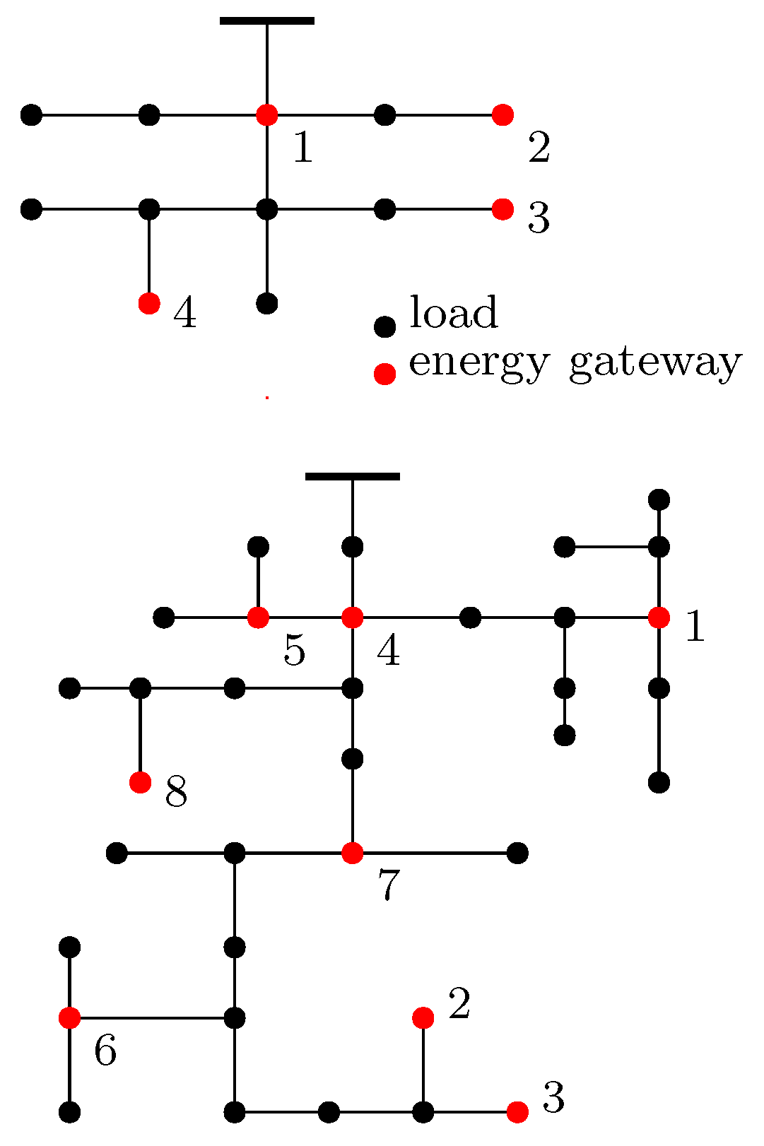
In this section, Algorithm I is applied and validated through numerical simulations considering one of the phases of the IEEE 13-bus and the 37-bus bus test feeders [37], reported for reference in Figure 5, assuming the system to be balanced and with loads equally distributed among the three phases of each node. Two different kinds of buses are deployed on the testbeds: regular load, behaving like passive power users, and energy gateways, who are endowed with generation capabilities and storage devices. Voltages are calculated using a non-linear standard solver throughout our tests [38], and the maximum tolerated voltage magnitude is set to $U_{max}=1.05$. MC control iterations take place once every $15\mathrm{s}$, while each EG measures its own voltage magnitude and in case performs the local voltage control once every $0.1\mathrm{s}$.

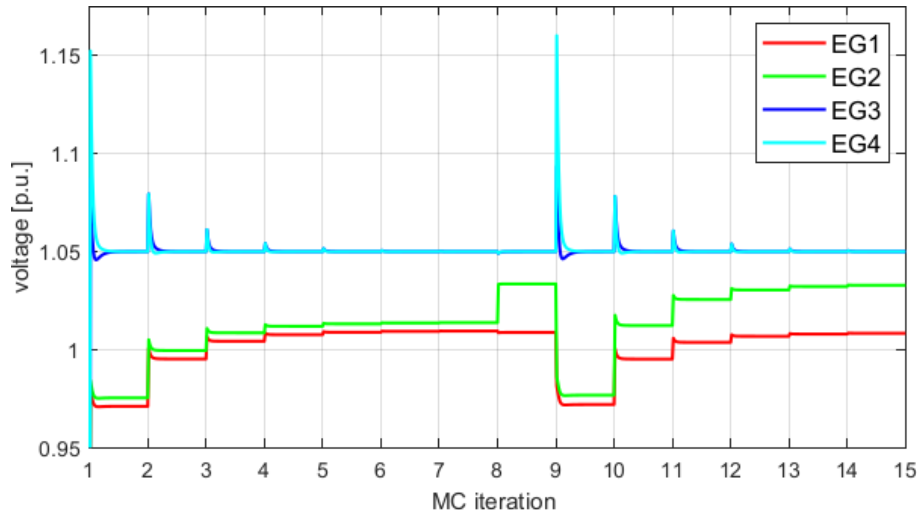
5.1. Static Load Scenario

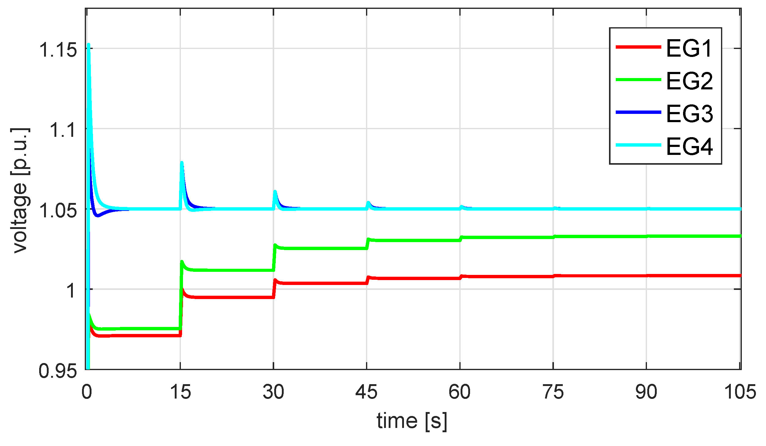
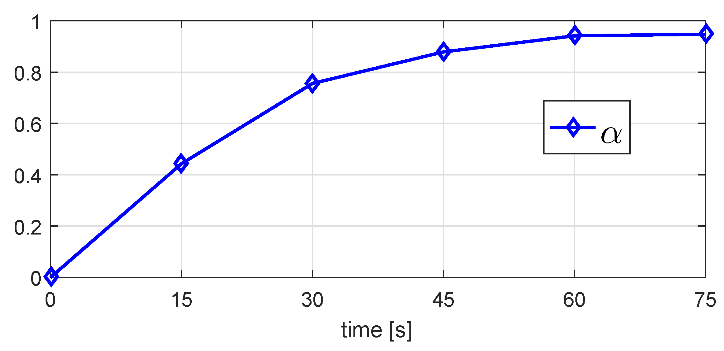
Firstly, Algorithm I is tested in a static load scenario, that is, with constant loads, in the IEEE 13-bus test feeder. Active and reactive power demands were set ranging from 110 to $300\mathrm{k}\mathrm{W}$, and from 60 to $200\mathrm{k}\mathrm{V}\mathrm{A}$. Four EGs are deployed in the distribution network. Every EG is endowed with a power generator, whose rated power output ranges from $0.9$ to $3\mathrm{M}\mathrm{W}$, and with an energy storage with capacity ranging from 100 to $300\mathrm{k}\mathrm{W}$. EG active power outputs are initially set to zero. Figure 6 and Figure 7 report the EG voltage magnitudes and the EG injected active powers, respectively. Noticeably, EG${}_3$ and EG${}_4$ experience several overvoltage situations, as displayed in Figure 6; however, voltage magnitudes are brought to the admissible limit by the local controller, by decreasing the active power EG${}_3$ and EG${}_4$ inject into the grid (i.e., $p_3$ and $p_4$). As a consequence, the centralized algorithm makes EG${}_1$ and EG${}_2$ increase their power injection $p_1$ and $p_3$ to meet the requirement of $p_0^{*}$, as displayed in Figure 7. Figure 8 reports the sequence of the broadcasted signal $\alpha \left(\ell \right)$. As stated in Proposition 1, the sequence converges monotonically to its limit value $\overline{\alpha }$.

5.2. Time-Varying Loads Scenario

Secondly, Algorithm I is tested on the IEEE 37-bus test feeder with time-varying load demand. Eight EGs are deployed in the distribution network, equipped with photovoltaic panels. To model household loads and solar generators power outputs, data retrieved from the Pecan Street project over 1 January 2013 are used [39]. For what concerns reactive power demand, power factors are drawn uniformly within 0.95 to 1 for every time interval, being that the Pecan Street dataset does not provide reactive power information. Finally, load demands are normalized so that their maxima matches the benchmark nominal values, ranging from 20 to $140\mathrm{k}\mathrm{W}$. EGs are also equipped with energy storage systems, whose power capacity ranged from 50 to $100\mathrm{k}\mathrm{W}$.

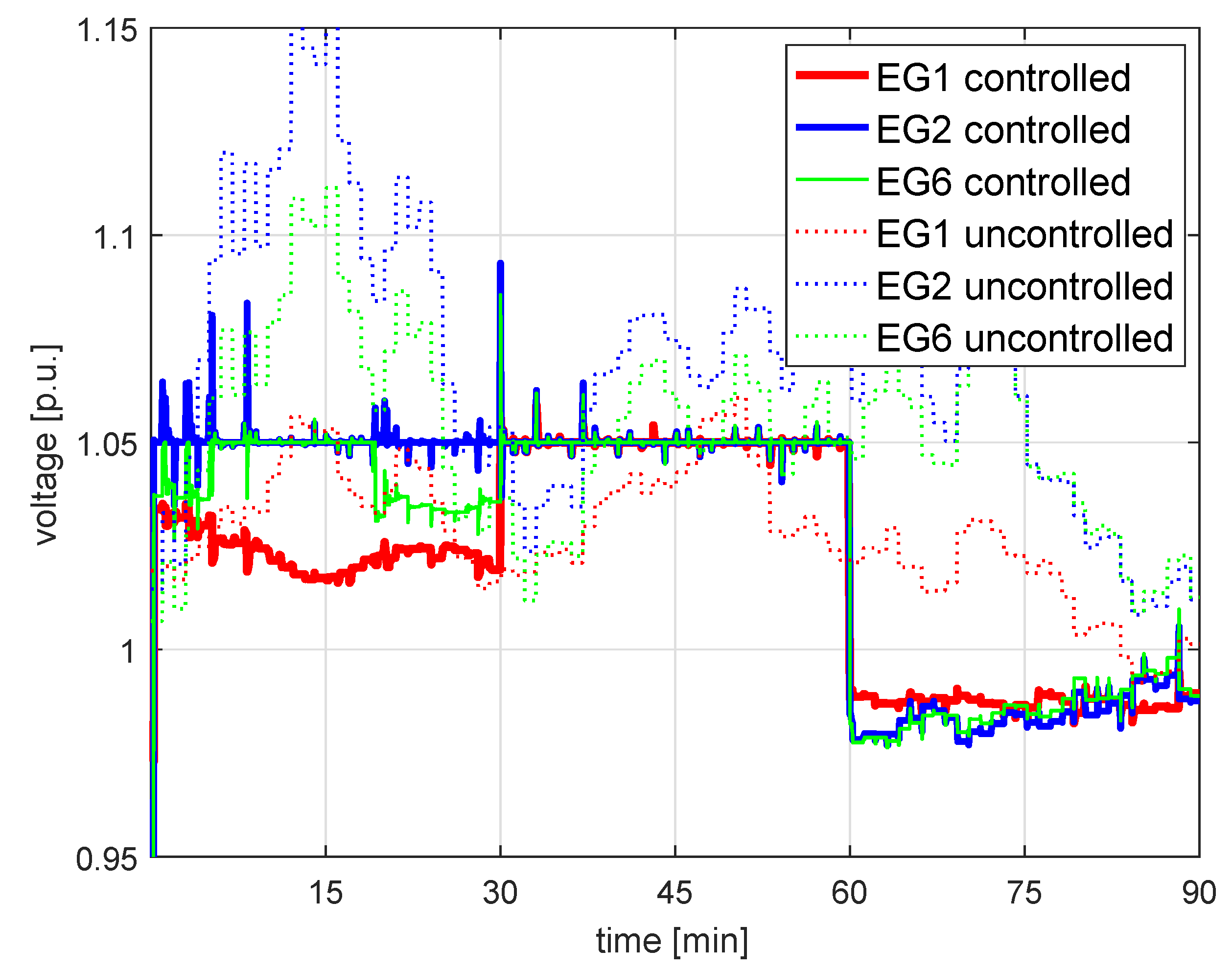
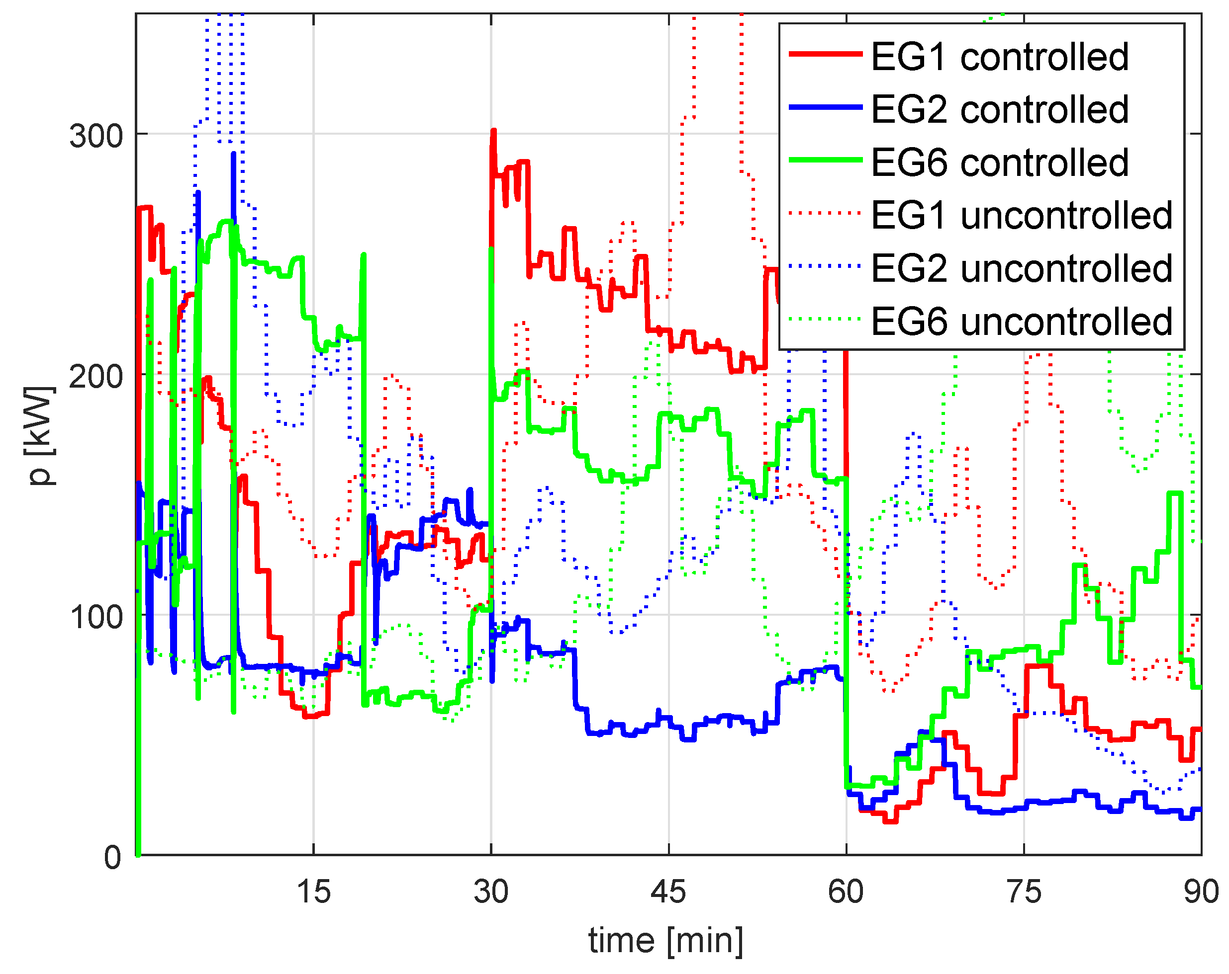
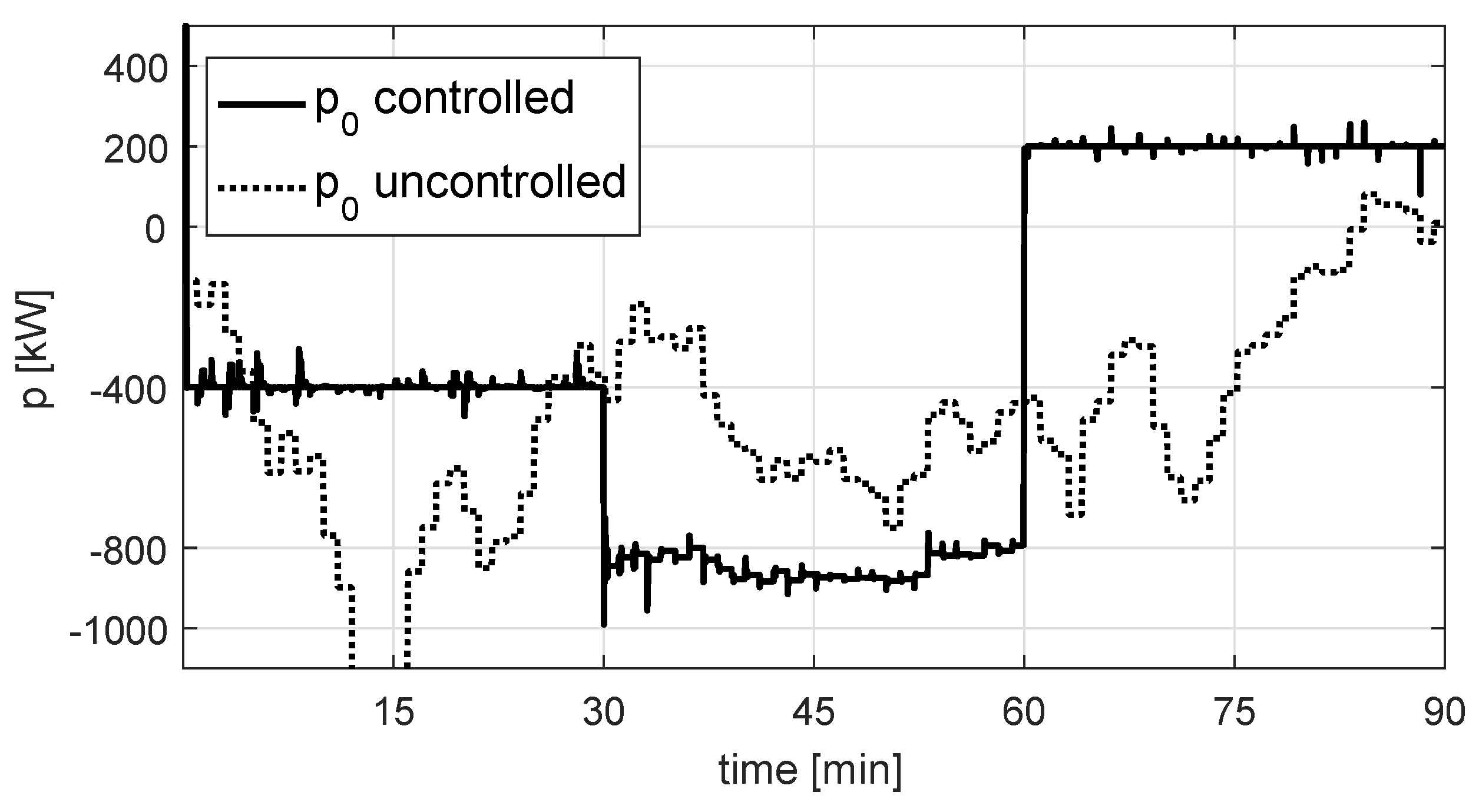
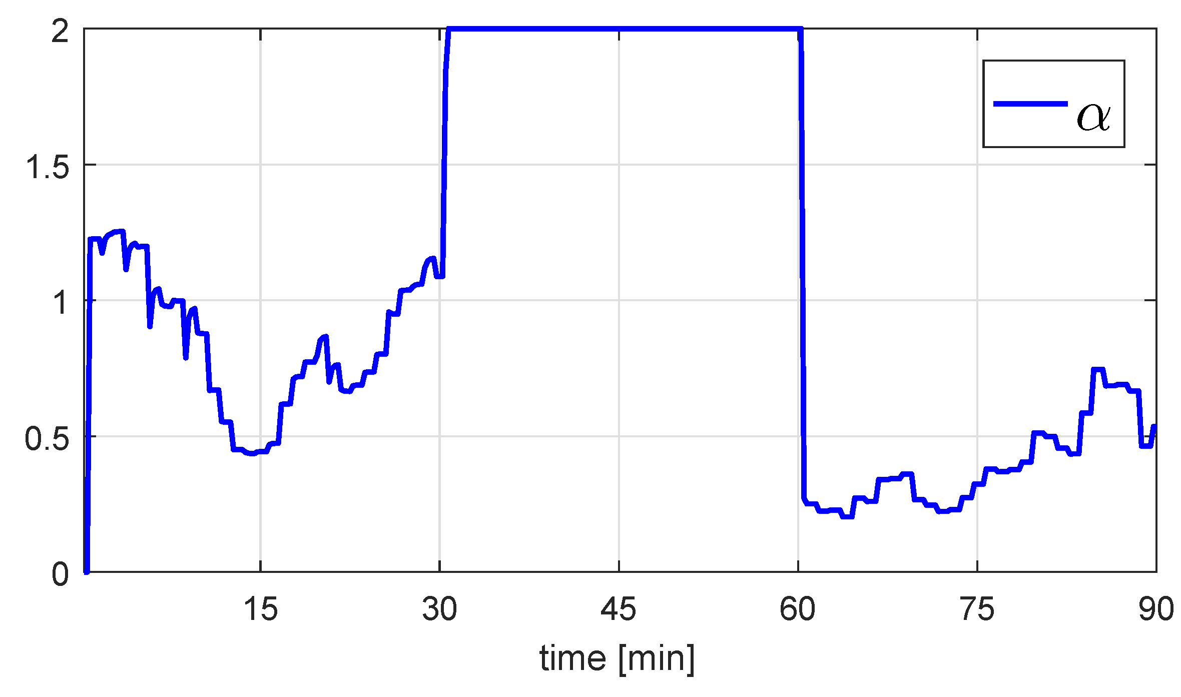
The simulated time window consists of $90\min$, and it is partitioned into three intervals, namely, $I_1$ covering the period 0–$30\min$; $I_2$ covering the period 30–$60\min$; and $I_3$ covering the period 60–$90\min$. Voltage magnitudes and power injections of some of the EGs and the power absorbed from the main grid are reported in Figure 9, Figure 10 and Figure 11, respectively, both in the case in which the network is controlled by Algorithm I and in the case of uncontrolled power injections. The sequence of the coefficients $\alpha$ generated by the control scheme is instead depicted in Figure 12.

During $I_1$, the control algorithm is able to provide to the external network the power required, set to $400\mathrm{k}\mathrm{W}$. Furthermore, the EGs voltage magnitudes are maintained within the desired interval. Note that, during $I_1$, the sequence $\left\{\alpha \right(\ell \left)\right\}$ assumed values both below and over 1. That is, to keep the value of $p_0\left(\ell \right)$ equal to $p_0{\left(\ell \right)}^{*}$, the EGs have to curtail or store the excess of generation and to exploit the local batteries power output.

In $I_2$ the MC is asked to send to the main grid $1000\mathrm{k}\mathrm{W}$, which transcends the availability of the network. This explains why the broadcast $\alpha \left(\ell \right)$ is always set to 2. In fact, note that the EGs voltage magnitudes are all at $U_{max}$, as a consequence of their power output. Hence, delivering more power would result in a further voltage increase and thus in the violation of the voltage constraint. In this situation, the EGs reached the limit of nodal injections ensuring the voltage constraints and cannot increase their power output.

During $I_3$, the network is supposed to absorb $200\mathrm{k}\mathrm{W}$ from the external grid. Again, to keep constant $p_0$, the MC enforced the EGs to not inject all the generated power, but rather either to store on energy storages or to curtail part of the available power.

The former numerical tests show that, apart from brief oscillations due to sudden load changes, Algorithm 1 satisfies the voltage magnitude constraints and meets, when it is possible, the power requirement. On the other hand, without the proposed control, not only is the requirement on $p_0$ not met but also the system experiences several and prolonged overvoltage situations.

5.3. Communication Failure Scenario

Finally, the case of communication failure between the MC and some of the EGs is considered. The proposed control scheme can adapt to this occurrence in the following way:

• EGs that are unreachable (i.e., not receiving new, updated coefficient $\alpha$) keep constant their power injections, unless their voltage exceeds the operational constraints. EGs experiencing overvoltage in this condition apply the local voltage control scheme;
• the MC computes and broadcasts the coefficient $\alpha$ based on the information gathered from the EGs that are reachable.

The former protocol was tested on the same load scenario considered in Section 5.1. In the example now reported, communication with EG${}_2$ and EG${}_3$ is lost from the 2-nd to the 7-th control cycle. During that period of time, EG${}_2$ keeps constant its power injections; on the other hand, EG${}_3$ performs the local control rule, having its voltage magnitude violating the operational constraints, see Figure 13 and Figure 14. Noticeably, during communication failure, EG${}_2$ and EG${}_3$ inject active power that subtract to the total load power, while not taking part to the control; automatically, the MC computes the coefficient $\alpha$ considering only the other EGs. Remarkably, the algorithm keeps capable of regulating the voltages and fulfilling the power requirements at the PCC. When communication is restored, EG${}_2$ and EG${}_3$ can participate again in the power sharing and their output power changes according to the values of $\alpha$. Dispatchability is guaranteed in steady-state along the considered sequence of events.

6. Conclusions

This paper presents and analyzes a simple approach for the control of distributed energy resources in low-voltage microgrids. The approach makes use of non-time-critical power data to be communicated from the active agents (i.e., nodes with energy resources) to a centralized controller by exploiting a communication means of limited bandwidth. The centralized controller broadcasts active power set-points to all the active nodes. The control of the power flow (taking place centrally, at the microgrid PCC) and the local overvoltage control (instead performed distributedly, at each EG) cooperate so that both the power flow at the PCC of the microgrid and the voltage magnitudes at the point of connection of the EGs can be simultaneously regulated; this is shown formally by mathematical analyses and by numerical simulations. The controller is tested by simulations referring to the IEEE test feeders in realistic configurations. The results show that the centralized power-based control succeeds in controlling the active power exchanged at PCC and avoids local overvoltages.

References

- Parhizi, S.; Lotfi, H.; Khodaei, A.; Bahramirad, S. State of the Art in Research on Microgrids: A Review. IEEE Access 2015, 3, 890–925. [Google Scholar] [CrossRef]
- Bullich-Massagué, E.; Díaz-González, F.; Aragüés-Peñalba, M.; Girbau-Llistuella, F.; Olivella-Rosell, P.; Sumper, A. Microgrid clustering architectures. Appl. Energy 2018, 212, 340–361. [Google Scholar] [CrossRef]
- Marnay, C.; Chatzivasileiadis, S.; Abbey, C.; Iravani, R.; Joos, G.; Lombardi, P.; Mancarella, P.; von Appen, J. Microgrid Evolution Roadmap. In Proceedings of the 2015 International Symposium on Smart Electric Distribution Systems and Technologies (EDST), Vienna, Austria, 8–11 September 2015; pp. 139–144. [Google Scholar] [CrossRef]
- Cornélusse, B.; Savelli, I.; Paoletti, S.; Giannitrapani, A.; Vicino, A. A community microgrid architecture with an internal local market. Appl. Energy 2019, 242, 547–560. [Google Scholar] [CrossRef] [Green Version]
- IEEE Standard for the Specification of Microgrid Controllers; IEEE Std 2030.7-2017; IEEE: Piscataway, NJ, USA, 2018; pp. 1–43.
- IEA. Overcoming PV Grid Issues in the Urban Areas; Technical Report IEA-PVPS T10-06-2009; IEA International Energy Agency: Paris, France, 2009. [Google Scholar]
- Katiraei, F.; Agüero, J. Solar PV Integration Challenges. IEEE Power Energy Mag. 2011, 9, 62–71. [Google Scholar] [CrossRef]
- Stadler, M.; Cardoso, G.; Mashayekh, S.; Forget, T.; DeForest, N.; Agarwal, A.; Schönbein, A. Value streams in microgrids: A literature review. Appl. Energy 2016, 162, 980–989. [Google Scholar] [CrossRef] [Green Version]
- Wang, J.; Zhao, C.; Pratt, A.; Baggu, M. Design of an advanced energy management system for microgrid control using a state machine. Appl. Energy 2018, 228, 2407–2421. [Google Scholar] [CrossRef]
- Molzahn, D.K.; Dörfler, F.; Sandberg, H.; Low, S.H.; Chakrabarti, S.; Baldick, R.; Lavaei, J. A Survey of Distributed Optimization and Control Algorithms for Electric Power Systems. IEEE Trans. Smart Grid 2017, 8, 2941–2962. [Google Scholar] [CrossRef]
- Eid, B.M.; Rahim, N.A.; Selvaraj, J.; El Khateb, A.H. Control Methods and Objectives for Electronically Coupled Distributed Energy Resources in Microgrids: A Review. IEEE Syst. J. 2016, 10, 446–458. [Google Scholar] [CrossRef]
- Han, Y.; Zhang, K.; Li, H.; Coelho, E.A.A.; Guerrero, J.M. MAS-Based Distributed Coordinated Control and Optimization in Microgrid and Microgrid Clusters: A Comprehensive Overview. IEEE Trans. Power Electron. 2018, 33, 6488–6508. [Google Scholar] [CrossRef]
- Mahmoud, M.; Hussain, S.A.; Abido, M. Modeling and control of microgrid: An overview. J. Frankl. Inst. 2014, 351, 2822–2859. [Google Scholar] [CrossRef]
- Serban, I. A control strategy for microgrids: Seamless transfer based on a leading inverter with supercapacitor energy storage system. Appl. Energy 2018, 221, 490–507. [Google Scholar] [CrossRef]
- Brandao, D.I.; de Araújo, L.S.; Caldognetto, T.; Pomilio, J.A. Coordinated control of three- and single-phase inverters coexisting in low-voltage microgrids. Appl. Energy 2018, 228, 2050–2060. [Google Scholar] [CrossRef]
- Guerrero, J.M.; Vasquez, J.C.; Matas, J.; de Vicuna, L.G.; Castilla, M. Hierarchical Control of Droop-Controlled AC and DC Microgrids - A General Approach Toward Standardization. IEEE Trans. Ind. Electron. 2011, 58, 158–172. [Google Scholar] [CrossRef]
- Simpson-Porco, J.; Shafiee, Q.; Dorfler, F.; Vasquez, J.; Guerrero, J.; Bullo, F. Secondary Frequency and Voltage Control of Islanded Microgrids via Distributed Averaging. Ind. Electron. IEEE Trans. 2015, 62, 7025–7038. [Google Scholar] [CrossRef]
- Schiffer, J.; Seel, T.; Raisch, J.; Sezi, T. Voltage Stability and Reactive Power Sharing in Inverter-Based Microgrids With Consensus-Based Distributed Voltage Control. IEEE Trans. Control Syst. Technol. 2016, 24, 96–109. [Google Scholar] [CrossRef]
- Riverso, S.; Tucci, M.; Vasquez, J.C.; Guerrero, J.M.; Ferrari-Trecate, G. Stabilizing plug-and-play regulators and secondary coordinated control for AC islanded microgrids with bus-connected topology. Appl. Energy 2018, 210, 914–924. [Google Scholar] [CrossRef]
- Tenti, P.; Costabeber, A.; Mattavelli, P.; Trombetti, D. Distribution Loss Minimization by Token Ring Control of Power Electronic Interfaces in Residential Microgrids. IEEE Trans. Ind. Electron. 2012, 59, 3817–3826. [Google Scholar] [CrossRef]
- Caldognetto, T.; Buso, S.; Tenti, P.; Brandao, D.I. Power-Based Control of Low-Voltage Microgrids. IEEE J. Emerg. Sel. Top. Power Electron. 2015, 3, 1056–1066. [Google Scholar] [CrossRef]
- Bolognani, S.; Zampieri, S. A Distributed Control Strategy for Reactive Power Compensation in Smart Microgrids. IEEE Trans. Autom. Control 2013, 58, 2818–2833. [Google Scholar] [CrossRef] [Green Version]
- Guerrero, J.M.; Matas, J.; de Vicuna, L.G.; Castilla, M.; Miret, J. Decentralized Control for Parallel Operation of Distributed Generation Inverters Using Resistive Output Impedance. IEEE Trans. Ind. Electron. 2007, 54, 994–1004. [Google Scholar] [CrossRef]
- Bolognani, S.; Zampieri, S. On the existence and linear approximation of the power flow solution in power distribution networks. IEEE Trans. Power Syst. 2015, 31, 163–172. [Google Scholar] [CrossRef]
- Viciana, E.; Alcayde, A.; Montoya, F.G.; Baños, R.; Arrabal-Campos, F.M.; Manzano-Agugliaro, F. An Open Hardware Design for Internet of Things Power Quality and Energy Saving Solutions. Sensors 2019, 19, 627. [Google Scholar] [CrossRef]
- Viciana, E.; Alcayde, A.; Montoya, F.G.; Baños, R.; Arrabal-Campos, F.M.; Zapata-Sierra, A.; Manzano-Agugliaro, F. OpenZmeter: An Efficient Low-Cost Energy Smart Meter and Power Quality Analyzer. Sustainability 2018, 10, 4038. [Google Scholar] [CrossRef]
- Angioni, A.; Sadu, A.; Ponci, F.; Monti, A.; Patel, D.; Williams, F.; Della Giustina, D.; Dede, A. Coordinated voltage control in distribution grids with LTE based communication infrastructure. In Proceedings of the IEEE 15th International Conference on Environment and Electrical Engineering (EEEIC), Rome, Italy, 10–13 June 2015; pp. 2090–2095. [Google Scholar] [CrossRef]
- IEEE Standard for Interconnecting Distributed Resources with Electric Power Systems; IEEE Std 1547-2003; IEEE: Piscataway, NJ, USA, 2003; Volume 28. [CrossRef]
- Rocabert, J.; Luna, A.; Blaabjerg, F.; Rodríguez, P. Control of Power Converters in AC Microgrids. IEEE Trans. Power Electron. 2012, 27, 4734–4749. [Google Scholar] [CrossRef]
- Carvalho, P.; Correia, P.F.; Ferreira, L. Distributed Reactive Power Generation Control for Voltage Rise Mitigation in Distribution Networks. IEEE Trans. Power Syst. 2008, 23, 766–772. [Google Scholar] [CrossRef]
- Bolognani, S.; Carli, R.; Cavraro, G.; Zampieri, S. Distributed reactive power feedback control for voltage regulation and loss minimization. Autom. Control. IEEE Trans. 2015, 60, 966–981. [Google Scholar] [CrossRef]
- Cavraro, G.; Carli, R. Algorithms for Voltage Control in Distribution Networks. In Proceedings of the IEEE International Conference on Smart Grid Communications (SmartGridComm 2015), Sydney, Australia, 6–9 November 2016. [Google Scholar]
- Tonkoski, R.; Lopes, L.; El-Fouly, T. Coordinated Active Power Curtailment of Grid Connected PV Inverters for Overvoltage Prevention. IEEE Trans. Sustain. Energy 2011, 2, 139–147. [Google Scholar] [CrossRef]
- Kabir, M.; Mishra, Y.; Ledwich, G.; Dong, Z.; Wong, K. Coordinated Control of Grid-Connected Photovoltaic Reactive Power and Battery Energy Storage Systems to Improve the Voltage Profile of a Residential Distribution Feeder. IEEE Trans. Ind. Inf. 2014, 10, 967–977. [Google Scholar] [CrossRef]
- Anurag, A.; Yang, Y.; Blaabjerg, F. Thermal Performance and Reliability Analysis of Single-Phase PV Inverters with Reactive Power Injection Outside Feed-In Operating Hours. IEEE J. Emerg. Sel. Top. Power Electron. 2015, in press. [Google Scholar] [CrossRef]
- Cavraro, G.; Kekatos, V. Inverter probing for power distribution network topology processing. arXiv 2018, arXiv:1802.06027. [Google Scholar] [CrossRef]
- Kersting, W.H. Radial distribution test feeders. IEEE Power Eng. Soc. Winter Meet. 2001, 2, 908–912. [Google Scholar] [CrossRef]
- Zimmerman, R.D.; Murillo-Sánchez, C.E.; Thomas, R.J. MATPOWER: Steady-state operations, planning and analysis tools for power systems research and education. IEEE Trans. Power Syst. 2011, 26, 12–19. [Google Scholar] [CrossRef]
- Pecan Street Inc. Dataport. Available online: Https://dataport.pecanstreet.org/ (accessed on 10 July 2019).
Figure 1.
Smart microgrid scenario.
Figure 2.
The considered master/slave microgrid architecture with the power-based control algorithm.
Figure 3.
Structure of an Energy Gateway (EG).
Figure 4.
Representation of the definition of the coefficient on the basis of local (4) and total availabilities (14) and the computed power reference (8).
Figure 5.
The IEEE 13-bus (top panel) and 37-bus (bottom panel) test feeder.
Figure 6.
Voltage magnitude of the EGs.
Figure 7.
Power injected by the EGs.
Figure 8.
Sequence of master controller (MC) broadcast .
Figure 9.
Figure 10.
Figure 11.
Figure 12.
Figure 13.
Voltage magnitude of the EGs during a communication failure affecting EG and EG in iterations 2-nd to 7-th.
Figure 14.
Power injected by the EGs during a communication failure affecting EG and EG in iterations 2nd to 7th.
© 2019 by the authors. Licensee MDPI, Basel, Switzerland. This article is an open access article distributed under the terms and conditions of the Creative Commons Attribution (CC BY) license (http://creativecommons.org/licenses/by/4.0/).
Share and Cite
MDPI and ACS Style
Cavraro, G.; Caldognetto, T.; Carli, R.; Tenti, P. A Master/Slave Approach to Power Flow and Overvoltage Control in Low-Voltage Microgrids. Energies 2019, 12, 2760. https://doi.org/10.3390/en12142760
AMA Style
Cavraro G, Caldognetto T, Carli R, Tenti P. A Master/Slave Approach to Power Flow and Overvoltage Control in Low-Voltage Microgrids. Energies. 2019; 12(14):2760. https://doi.org/10.3390/en12142760
Chicago/Turabian StyleCavraro, Guido, Tommaso Caldognetto, Ruggero Carli, and Paolo Tenti. 2019. "A Master/Slave Approach to Power Flow and Overvoltage Control in Low-Voltage Microgrids" Energies 12, no. 14: 2760. https://doi.org/10.3390/en12142760
Note that from the first issue of 2016, this journal uses article numbers instead of page numbers. See further details here.