Fuzzy Neural Network Control of Thermostatically Controlled Loads for Demand-Side Frequency Regulation


School of Electrical Engineering, Yanshan University, Qinhuangdao 066004, China
*
Author to whom correspondence should be addressed.
Energies 2019, 12(13), 2463; https://doi.org/10.3390/en12132463
Submission received: 4 June 2019
/
Revised: 20 June 2019
/
Accepted: 24 June 2019
/
Published: 26 June 2019
(This article belongs to the Special Issue Applied Neural Networks and Fuzzy Logic in Power Electronics, Motor Drives, Renewable Energy Systems and Smart Grids)
Abstract
:In this paper, a fuzzy neural network controller for regulating demand-side thermostatically controlled loads (TCLs) is designed with the aim of stabilizing the frequency of the smart grid. Specifically, the balance between power supply and demand is achieved by tracking the automatic generation control (AGC) signal in an electric power system. The particle swarm optimization (PSO) and error back propagation (BP) algorithms are used to optimize the control parameters and consequently reduce the tracking errors. The fuzzy neural network can be applied to solve load control problems in power systems, since its self-learning and associative storage functions can deal with the highly nonlinear relationship between input and output. Simulation results show the advantage of the fuzzy neural network control scheme in terms of frequency regulation error and consumer comfort.
1. Introduction
Smart grid is a modern grid infrastructure with high efficiency, reliability, and safety, which is based on renewable energy, automatic control, and modern communication technology [1,2]. An ancillary service is indispensable in an electric service, and plays a vital role in providing strong support for power transmission and power system operation. Ancillary service includes services related to frequency stability. The stability of grid frequency is closely related to the operation of power market and the equipment safety of the power generation side and power consumption side. Ancillary service mainly includes: Frequency adjustment, automatic generation control, spinning reserve, and peaking services.
The mismatch between the power supply side and the area power consumption can affect the frequency of the power system. Hence, the load frequency regulation is necessary in power systems, in order to maintain power balance under normal conditions [3]. Grid frequency can be used to evaluate power quality. The main way to adjust the frequency of the power system is to change the generated output power and manage the loads in demand side. Reasonable control of temperature control loads can provide adjustable buffer energy for power systems [4]. A great deal of potential electrically-thermal energy is stored in all sorts of heat buffers equipment, such as heating, air conditioning units, and fridges [5]. The advantages of aggregated thermostatically controlled loads (TCLs) to take part in power grid frequency regulation are as follows: Firstly, the TCLs which can store massive energy are of wide distributions; secondly, the control method of them is simple, fast, and real-time; thirdly, the aggregated TCLs can generate a continuous reaction without considering the discrete characteristics of the individual load control [6]. The management of TCLs is one of frequency adjustment strategies with extremely high feasibility to ensure frequency stability and improve power quality.
Recently, the bilinear partial differential equation (PDE) model was developed to provide effective control of aggregated TCLs [7]. Two control methods, based on the combination of estimator and controller, were utilized to control TCLs and effectively track demand curve [8]. A centralized and distributed algorithm based on the state space model of heating ventilation and air-conditioning (HVAC) was proposed to reduce power fluctuations and improve satisfaction of demand side [9]. A model predictive control was described and applied to demand-side response services in [10]. A distributed model predictive control (DMPC) method based on an optimized aggregation model was applied to provide frequency regulation services [11]. A Fokker–Planck diffusion model and a direct load control algorithm were developed in [12]. A model of aggregate homogeneous TCLs with uniform variation of temperature set-point was developed, and a linear quadratic regulator (LQR) has been designed in [13]. In [14], the authors proposed a novel causal method based on a parametric second-order model to forecast the energy conservation. In [15], a linear optimization model was built to provide frequency regulation services for power systems while also providing short-term demand response management. In [16], the authors proposed several switched control strategies for aggregate HVACs to provide demand-side frequency regulation. Although various aggregation characteristics of TCLs have been extensively studied, modeling precision still needs to be farther improved. As a matter of fact, it is hard to establish accurate mathematical models or physical models for aggregated TCLs because of various assumptions and computational complexity in the modeling process.
In recent years, artificial intelligence has developed rapidly with the characteristics of bionics and intelligence. This paper proposes a fuzzy neural network control method which adjusts TCLs based on the input and output data of TCLs instead of the aggregated TCL model. This method can reduce tracking errors and computational complexity, because it draws the advantages–logic reasoning capability of fuzzy control and self-learning capability of the neural network [17]. This study has the following contributions:
- The fuzzy neural network can model the characteristics of aggregated TCLs in the network weight after training, which can meet the response of the system input and output without modeling the load characteristics.
- The combination of particle swarm optimization (PSO) and back propagation (BP) algorithms, which optimize the initial value of weight and membership degree parameters, can avoid the local minimum and accelerate effectively to convergence speed.
The rest of this paper is organized as follows. Section 1 introduces the thermal dynamics of individual TCLs and the frequency regulation problem. Section 2 describes the system structure, algorithm, and optimization of the fuzzy neural network control in detail. The simulation results are shown in Section 3. Finally, the conclusions are summarized in Section 4.
2. Problem Formulation
2.1. Individual TCL Characteristic
The TCLs can consume electric energy and release thermal energy, which can usually be stored and transferred [18]. For example, the simple TCLs usually have two work states, i.e., “on” or “off”, and each corresponds to one power value, i.e., or 0. When there is excess power in generation side, the TCL is changed to the “on” state, then the electricity consumption increases and the transformed heat energy will also increase. When the power generation fails to meet users’ needs, the TCLs are changed to the “off” state and the power demand will be reduced in order to stabilize the power grid frequency. The characteristics are described as follows [19]:
where T and represent the indoor and outdoor temperature, respectively. P, R, and C denote energy transfer rate, thermal resistance, and thermal capacitance, respectively. represents the switching state of loads.
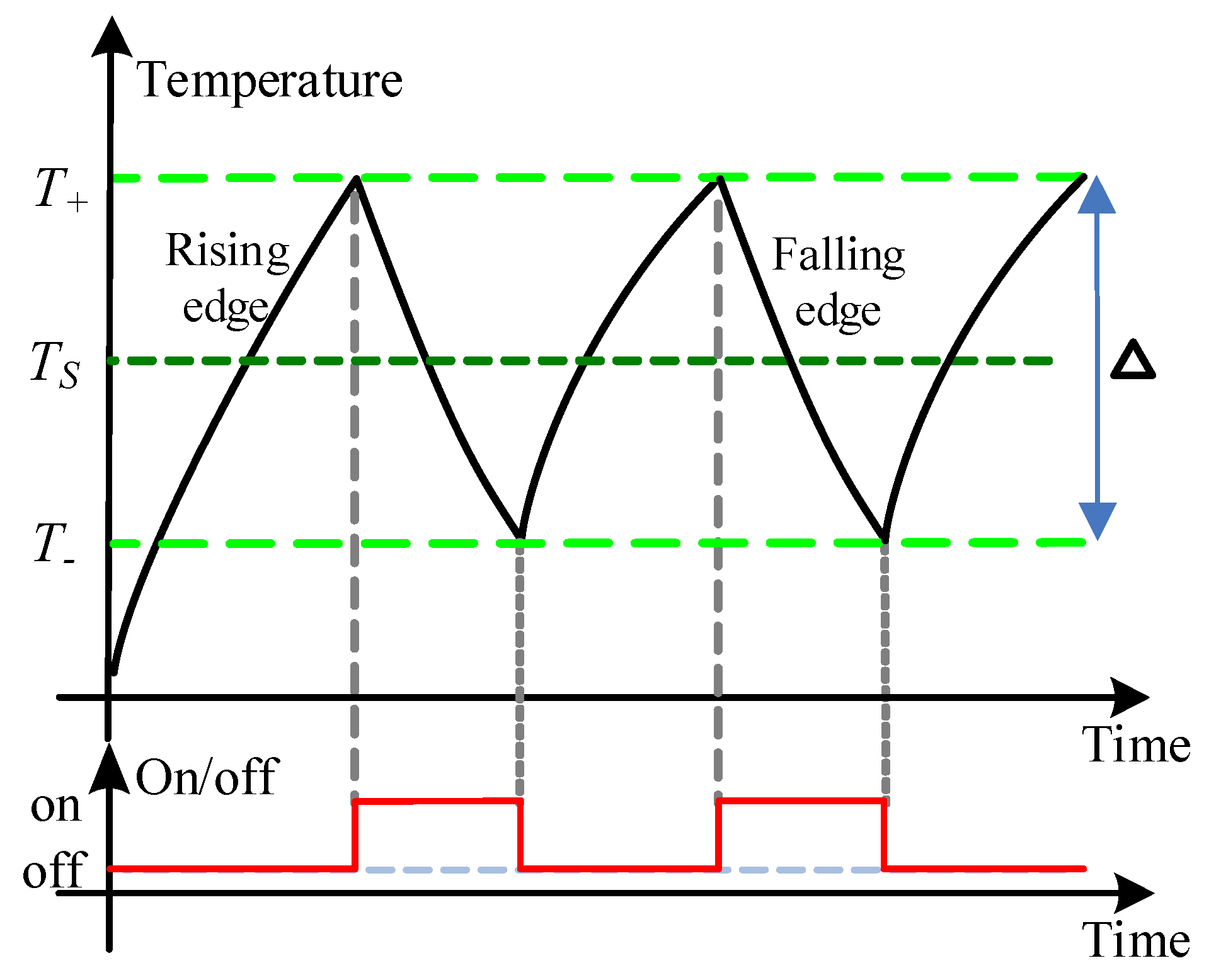
The operation characteristics of an individual TCL are shown in Figure 1 and Figure 2. The set-point regulation method is adopted for regulating TCLs to achieve the purpose of peak shaving and load shifting. In the figure, u is the temperature set-point change. , , and on the left of the figure denote the upper boundary of temperature, the temperature set-point, and the lower boundary of temperature, respectively. is the width of the temperature deadband, which denotes the difference between the upper and lower limits of temperature. According to the physical characteristics of TCLs, , , , and have the following relationship:
The rising edge represents that the room temperature has a rise caused by a natural heat conduction process when the TCL is off. The falling edge denotes the temperature drops caused by the cooling process of the TCL when the TCL is turned on. In order to keep the room temperature near the temperature set-point, the TCL will be changed from an off to an on state when the temperature reaches the upper limit and changed from on to off state when the temperature reaches the lower limit in Figure 1. We can observe that the upper and lower bounds of temperature vary with the temperature set-point, but the deadband keeps constant in Figure 2. Hence, when the temperature set-point changes, the TCL’s switch state can be indirectly changed, and the TCL’s running time will be extended or shortened. Therefore, prolonging or shortening the running time of TCL will change the demand-side power consumption, thus it is effective to maintain the stability of the power grid frequency.
Suppose that N TCLs are used to provide the frequency regulation. When u is changed, the power consumption in demand side will be shifted, which contributes to the peak shaving and valley filling for the grid. The aggregated power consumption could be expressed by
where (>1) is the efficiency coefficient of the ith TCL. is a binary variable. The TCL is on when ; and off when . denotes the rated power of the ith load.
2.2. Frequency Regulation Problem
In the power system, since the power is difficult to store in large quantities, the real-time power balance between the generation side and the demand side must be maintained which can achieve the goal of suppressing the grid frequency fluctuations, keeping the reliable power supply, avoiding accidents and hurting the user power equipment [20,21]. The aggregated TCLs can reliably provide the frequency regulation service by energy storage and flexible scheduling, which are mentioned by demand-side management. In that case, the power consumption of the TCLs tracks the frequency modulation power signal of the power grid by an effective controller and a control algorithm.
The frequency regulation signal , which is a continuous change of positive and negative power signals and reflects the supply and demand deviation, thus, needs to stacked on a baseline load signal —that will generate the actual tracking signal , which can be tracked by the aggregated TCLs. Here, is selected as the rated power at one temperature set-point. It can be described as:
where N represents that the quantity of TCLs.
From Figure 3, we can observe that the inputs of the controller are the difference between the actual tracking signal and the power consumption , which are the tracking error signal and its differential . The controller output is the temperature set-point change u. In the control scheme, since the fuzzy neural network controller looks like a black box with brilliant self-learning and self-adaptive ability, we do not need to model the aggregated TCLs. The fuzzy neural network can be trained to encode the internal characteristics of the controlled object into the initial value of the connection weight. The connection of BP and PSO algorithm is also used to optimize the parameters of the controller and achieve the goal of reducing load tracking errors, improving tracking performance of the power grid frequency signal, and providing better frequency regulation service.
3. Fuzzy Neural Network Control Scheme
3.1. Fuzzy Neural Network Structure
The fuzzy neural network structure established in this paper has four layers, each layer is connected by weighted values. The multi-layer forward fuzzy neural network has the following advantages and characteristics for automatic control:
- The network can realize any complex nonlinear mapping. In this paper, there is a nonlinear relationship between the real-time tracking error and the temperature set-point, which is not easy to be formulated. Therefore, the network essentially implements a mapping function from input to output, which is especially suitable for solving complicated internal mechanism problems;
- The network has strong self-learning ability. First, it can learn the nonlinear relationship between the real-time tracking error and the temperature set-point—that is, the training process—then it can reflect the extracted “reasonable” solving rules to the connection coefficients between the layers. The appropriate connection coefficient has great influence on the control effect for frequency regulation;
- The network has certain promotion and generalization ability.
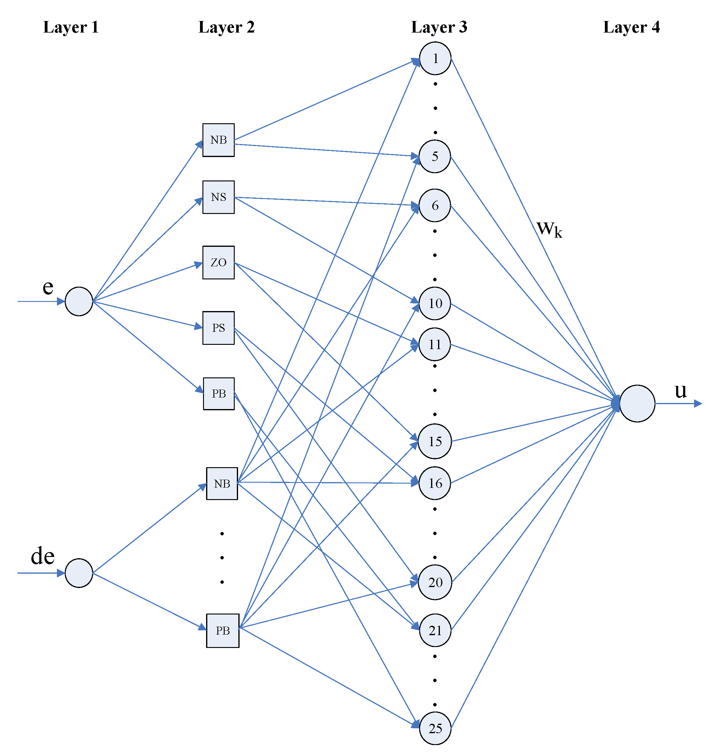
BP algorithm is adopted in the fuzzy neural network, its main feature is the forward transmission of the signal and the backward propagation of the error [22]. Since the transfer functions must satisfy the conditions of being differentiable everywhere, the hidden layer transfer function and the output layer activation function are Gaussian function and linear function, respectively. Fuzzy neural network mainly refers to the use of neural network structure to achieve fuzzy logic reasoning. Compared with a traditional neural network, the second layer can give specific physical meaning to tracking error, and the third layer is the fuzzy logic reasoning layer in the design of fuzzy neural network. The structure of the fuzzy neural network is shown in Figure 4 [23].
We define the error e and the error variation as fuzzy linguistic variables, and these two fuzzy language variables contain five linguistic values, i.e., NB, NS, ZO, PS, and PB. Thus, there are 25 rules in the third layer of the fuzzy neural network structure. In the following, represents the ith input of layer k, and represents the net input of the jth node of layer k, and represents the output of the jth node of layer k. The input and output relationships of each layer node are as follows [24,25]:
The fuzzy neural network has input layer, membership function layer, rule layer, and output layer from left to right in Figure 4. The input–output relationship in the input layer is
The membership function layer is used to evaluate membership degree of each input component which belongs to the fuzzy set of each linguistic variable. The input–output relationship of this layer is
where represents the input of the jth fuzzy set of the ith fuzzy variable. For the same fuzzy concept, the membership functions can be different. Although the form is not exactly the same, the functions follow normal distribution which can reflect the fuzzy information that is processed by fuzzy concept when solving problems. For example, if the membership function of normal distribution is adopted, the result is shown as follows:
where and are parameters of Gauss membership function of x. Hence, the input and output relationships of the second layer nodes are shown as
The third layer denotes fuzzy rule sets, every node denotes a fuzzy rule. This layer has 25 nodes. The input–output relationships of the third layer nodes are shown in Equations (15) and (16):
The fourth layer denotes controller output, i.e., the optimal result obtained by fuzzy neural network:
where denotes the temperature set-point change u.
3.2. Fuzzy Neural Network Learning Algorithm
Compared with other traditional methods, the BP algorithm has better persistence and predictability. In BP neural network, the error signal is transmitted backward from the output layer to the first layer. Therefore, hierarchical calculation can be reserved and the index function can be defined as:
where d is desired signal , and denotes in this paper.
If the output layer is concerned, we can draw the following Equations (20) from (15) and (16):
where represents the local gradient of the BP neural network. Since is unknown, we approximately replace it with the symbolic operator , and the learning rate in the following can compensate the inaccurate calculation form.The fundamentals of the BP neural network is to use the gradient descent method to correct the weights, and Equation (21) is obtained from Equation (20):
where .
For the fuzzy rule layer and the membership function layer, the local gradients are denoted as
where , k () stands for the node in the third layer, which are connected with the jth node in the second layer. i denotes another node in the second layer that is connected to the kth node in the third layer.
Therefore, the parameter correction value of the input membership function is as follows:
Finally, the correction algorithm of adjustable parameters in fuzzy neural networks is expressed by
where are learning rates for each adjustable parameter, and are momentum factors for each adjustable parameter. The well-chosen learning factors and momentum factors can accelerate algorithm convergence, reduce shock, and effectively suppress the local minimum—and their values are limited to interval.
3.3. Optimization of Initial Value of Adjustable Parameters
The learning effect of the fuzzy neural network has a strong dependence on the initial values of the connection weight and membership function. The BP algorithm is suitable for solving the complicated nonlinear problem, but the algorithm usually falls into local minimum, resulting in training failure. In [26], the authors proposed a method for estimating the parameters of dynamic models for induction motor dominating loads. Based on PSO, the method finds the adequate set of parameters that best fit the sampling data from the measurement for a period of time, minimizing the error of the outputs and active and reactive power demands. Hence, a hybrid algorithm uniting the PSO and BP algorithms was proposed to find the optimal initial parameter. The PSO algorithm includes a group of particles, these particles are stochastically distributed in the high-dimensional search space. These particles are group members that are used to find the optimal solution in a high-dimensional search space, and the optimal solution is equal to the possible position for the object. Each particle is a candidate optimal solution in a higher dimensional search space, the optimal direction and speed of individual particles are dependent on the optimal location and optimal speed of the whole particle and its own, and the optimization results are measured by the fitness function. The fitness function is determined by the specific problem. The mathematical description is as follows:
where , and denote the velocity, location, and historical optimal location of the ith particle, respectively. is the best position of all particles at present. and are learning rates, and and are two random numbers between 0 and 1.
Next, the root-mean-square error (RMSE) is defined as an indicator used to assess tracking performance, which can be defined as follows:
where denotes quantity of control cycles, and denote the upper and lower limits of the target signal range, respectively. The flow chart of the optimization algorithm is shown in Figure 5.
4. Simulation Results
In the simulations, the HVAC units track the daily automatic generation control (AGC) signal from the PJM (Pennsylvania–New Jersey Maryland Interconnection) electricity markets. Following the parameters of TCLs in the simulation process [7], it is assumed that the average values of R, C, and P in Equation (1) follow a Gaussian distribution with standard deviation 0.1, and the values of R, C, and P are 2 kW, 2 kWh, and 14 kWh, respectively. Assume the loads’ initial temperatures are distributed uniformly in the deadband of temperature, is 20 C and is 32 C. The deadband of temperature is C, in Equation (4) is , and the sampling time interval is 4 s. The tracking errors are used to characterize the performance of the frequency regulation based on the fuzzy neural network control.
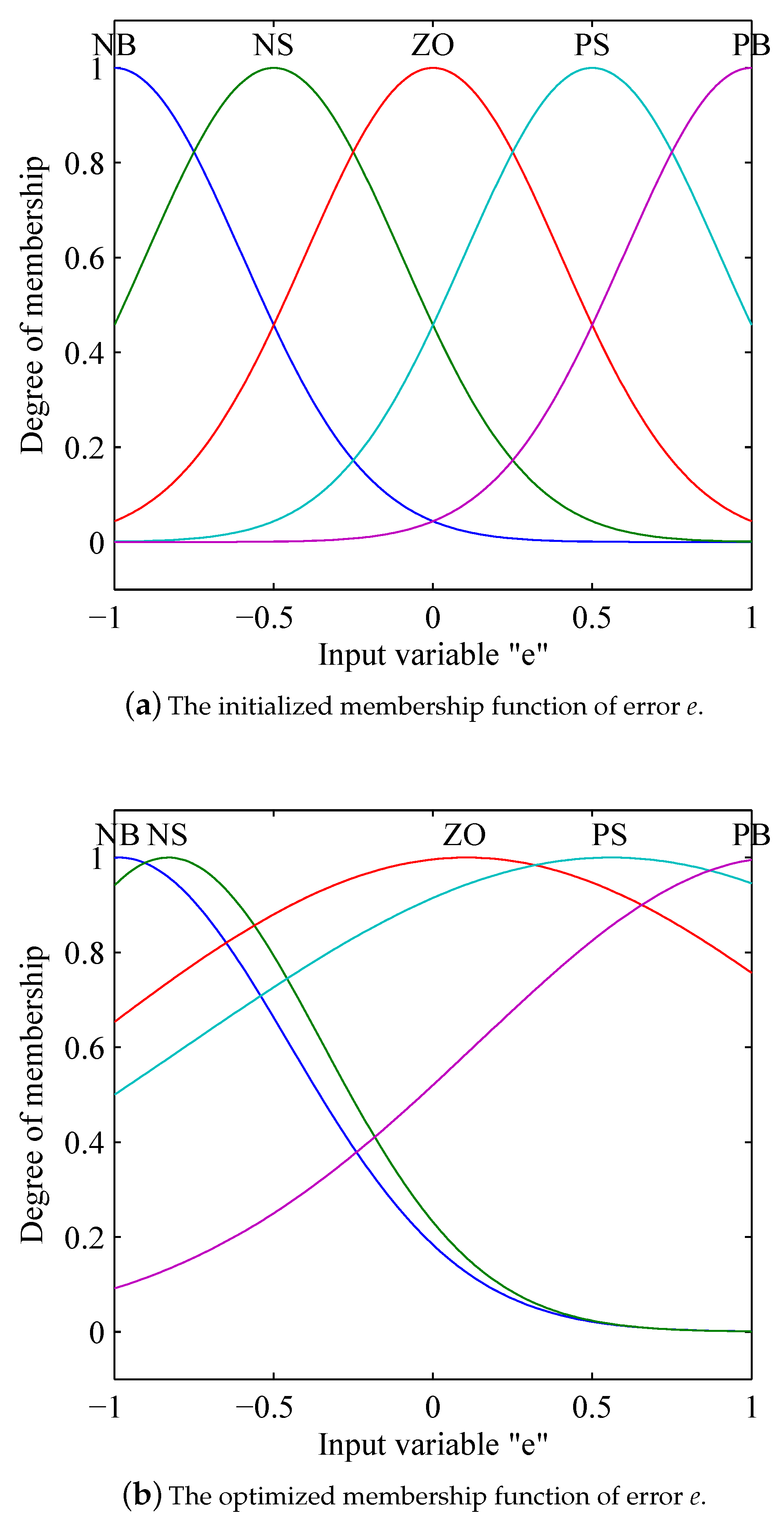
Through the iterative solution of the particle swarm optimization algorithm and BP algorithm, the appropriate connection weight coefficient is obtained after the training of 2500 sample dates. The membership functions of error e and error variation are shown in Figure 6 and Figure 7, respectively. At the beginning of the simulation, we assume that the membership functions of the fuzzy sets of error e and error variation are Gaussian functions, as shown in Figure 6a and Figure 7a—after training, the membership functions of each fuzzy set of the fuzzy neural network are shown in Figure 6b and Figure 7b.
The influence of the PSO algorithm on the performance of the neural fuzzy network is shown in Figure 8. From the results shown in Figure 8, it can be observed that the RMSE with optimized parameter under PSO algorithm is 2.7003, which is obviously smaller than the RMSE with random parameters. Hence, it is necessary to optimize these parameters by the PSO algorithm.
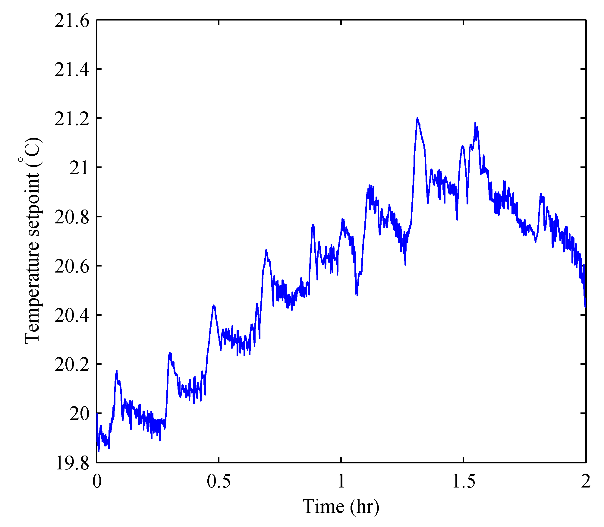
The control performance of the fuzzy neural network is shown in Figure 9, and the changes in temperature set-point are shown in Figure 10. We observe that the aggregated TCLs can track the AGC signal in a power system to provide ancillary service, and the maximum change in temperature set-point is C, which indicates that the control scheme has a minor impact on the thermal comfort of consumers.
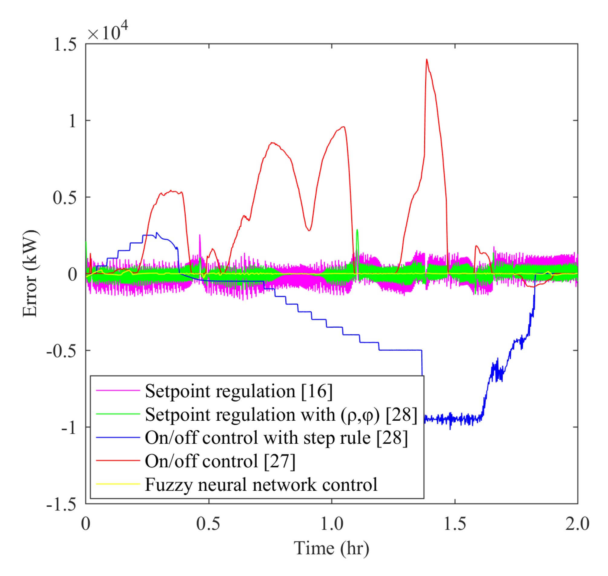
Furthermore, several control strategies are compared for the problems of frequency control. Figure 11 shows the comparison results of tracking errors, it is shown that the fuzzy neural network control strategy can better reduce the tracking errors. Table 1 shows the detailed comparison results, which demonstrate that the fuzzy neural network control strategy can better reduce tracking errors with acceptable temperature set-point change. In addition, it can be observed from Table 1 that there are a small number of switching on/off times using the fuzzy neural network control strategy, which indicates that its regulation has a smaller impact on the life of TCLs compared with other control strategies.
5. Conclusions
In this paper, the frequency regulation method—based on fuzzy neural network control—is proposed to regulate the temperature set-point of TCLs in the ancillary service market. Due to the strong dependence of tracking accuracy on membership functions and connection weight coefficients, the combination of offline hybrid algorithms and online BP algorithms can better optimize the control parameters. Finally, the conclusion obtained from the simulation results is that the fuzzy neural network control has prominent advantages of tracking accuracy without modeling the aggregated TCLs.
Author Contributions
K.M. contributed the idea; Z.Q. wrote the paper; C.X. conceived and designed the experiments; Z.J. provided the software.
Funding
This work was supported by the National Key Research and Development Program of China under Grant 2016YFF0200105 and National Natural Science Foundation of China under Grant 61573303.
Conflicts of Interest
The authors declare no conflict of interest. The founding sponsors had no role in the design of the study; in the collection, analyses, or interpretation of data; in the writing of the manuscript, and in the decision to publish the results.
References
- Ma, K.; Liu, X.; Liu, Z.; Chen, C.; Liang, H.; Guan, X. Cooperative relaying strategies for smart grid communications: bargaining models and solutions. IEEE Internet Thing. J. 2017, 4, 2315–2325. [Google Scholar] [CrossRef]
- Hashemi-Dezaki, H.; Askarian-Abyaneh, H.; Haeri-Khiavi, H. Impacts of direct cyber-power interdependencies on smart grid reliability under various penetration levels of microturbine/wind/solar distributed generations. IET Gener. Trans. Distrib. 2016, 10, 928–937. [Google Scholar] [CrossRef]
- Wen, G.; Hu, G.; Hu, J.; Shi, X.; Chen, G. Frequency regulation of source-grid-load systems: A compound control strategy. IEEE Trans. Ind. Inf. 2016, 12, 69–78. [Google Scholar]
- Wang, D.; Jia, H.; Wang, C.; Lu, N. Performance evaluation of controlling thermostatically controlled appliances as virtual generators using comfort-constrained state-queueing models. IET Gener. Trans. Distrib. 2009, 8, 591–599. [Google Scholar] [CrossRef]
- Lu, N.; Vanouni, M. Passive energy storage using distributed electric loads with thermal storage. J. Mod. Power Syst. Clean Energy 2013, 1, 264–274. [Google Scholar] [CrossRef] [Green Version]
- Ma, K.; Hu, G.Q.; Spanos, C.J. Energy management considering load operations and forecast errors with application to HVAC systems. IEEE Trans. Smart Grid 2018, 9, 605–614. [Google Scholar] [CrossRef]
- Bashash, S.; Fathy, H.K. Modeling and control insights into demand-side energy management through setpoint control of thermostatic loads. In Proceedings of the American Control Conference (ACC), San Francisco, CA, USA, 29 June–1 July 2011; pp. 4546–4553. [Google Scholar]
- Ledva, G.S.; Vrettos, E.; Mastellone, S.; Andersson, G.; Mathieu, J.L. Managing communication delays and model error in demand response for frequency regulation. IEEE Trans. Power Syst. 2018, 33, 1299–1308. [Google Scholar] [CrossRef]
- Zhou, K.; Cai, L. A dynamic water-filling method for real-time HVAC load control based on model predictive control. IEEE Trans. Power Syst. 2013, 30, 1405–1414. [Google Scholar] [CrossRef]
- Mahdavi, N.; Braslavsky, J.H.; Seron, M.M.; West, S.R. Model predictive control of distributed air-conditioning loads to compensate fluctuations in solar power. IEEE Trans. Smart Grid 2017, 8, 3055–3065. [Google Scholar] [CrossRef]
- Liu, M.; Shi, Y.; Liu, X. Distributed MPC of aggregated heterogeneous thermostatically controlled loads in smart grid. IEEE Trans. Ind. Electron. 2016, 63, 1120–1129. [Google Scholar] [CrossRef]
- Callaway, D.S. Tapping the energy storage potential in electric loads to deliver load following and regulation, with application to wind energy. Energy Convers. Manag. 2009, 50, 1389–1400. [Google Scholar] [CrossRef] [Green Version]
- Kundu, S.; Sinitsyn, N.; Backhaus, S.; Hiskens, I. Modeling and control of thermostatically controlled loads. In Proceedings of the Power Systems Computation Conference, Stokholm, Sweden, 22–26 August 2011; Available online: https://arxiv.org/abs/1101.2157 (accessed on 25 June 2019).
- Perfumo, C.; Braslavsky, J.H.; Ward, J.K. Model-Based Estimation of Energy Savings in Load Control Events for Thermostatically Controlled Loads. IEEE Trans. Smart Grid 2014, 5, 1410–1420. [Google Scholar] [CrossRef] [Green Version]
- Trovato, V.; Tindemans, S.H.; Strbac, G. Leaky storage model for optimal multi-service allocation of thermostatic loads. IET Gener. Trans. Distrib. 2015, 10, 585–593. [Google Scholar] [CrossRef]
- Ma, K.; Yuan, C.; Yang, J.; Liu, Z.; Guan, X. Switched Control Strategies of Aggregated Commercial HVAC Systems for Demand Response in Smart Grids. Energies 2017, 10, 953. [Google Scholar] [CrossRef]
- Ni, Z.; Wang, M. Research on the Fuzzy Neural Network PID Control of Load Simulator Based on Friction Torque Compensation. In Proceedings of the Sixth International Conference on Intelligent Human-Machine Systems and Cybernetics, Hangzhou, China, 26–27 August 2014. [Google Scholar]
- Garcia-Valle, R.; Silva, L.C.P.D.; Xu, Z.; Ostergaard, J.J. Smart demand for improving short-term voltage control on distribution networks. IET Gener. Trans. Distrib. 2009, 3, 724–732. [Google Scholar] [CrossRef] [Green Version]
- Wai, C.H.; Beaudin, M.; Zareipour, H.; Schellenberg, A.; Lu, N. Cooling devices in demand response: A comparison of control methods. IEEE Trans. Smart Grid 2014, 6, 249–260. [Google Scholar] [CrossRef]
- Ma, K.; Hu, G.Q.; Spanos, C.J. Distributed Energy Consumption Control via Real-Time Pricing Feedback in Smart Grid. IEEE Trans. Control Syst. Technol. 2014, 22, 1907–1914. [Google Scholar] [CrossRef] [Green Version]
- Ma, K.; Wang, C.; Yang, J.; Hua, C.; Guan, X. Pricing mechanism with noncooperative game and revenue sharing contract in electricity market. IEEE Trans. Cybern. 2017, 49, 97–106. [Google Scholar] [CrossRef]
- Lin, F.J.; Shieh, P.H.; Hung, Y.C. An intelligent control for linear ultrasonic motor using interval type-2 fuzzy neural network. IET Electr. Power Appl. 2018, 2, 32–41. [Google Scholar] [CrossRef]
- Chen, Y.C.; Teng, C.C. A model reference control structure using a fuzzy neural network. Fuzzy Sets Syst. 1995, 73, 291–312. [Google Scholar] [CrossRef]
- Kong, S.G.; Kosko, B. Adaptive fuzzy systems for backing up a truck-and-trailer. IEEE Trans. Neural Netw. 1992, 3, 211–223. [Google Scholar] [CrossRef]
- Berenji, H.R.; Khedkar, P. Learning and tuning fuzzy logic controllers through reinforcements. IEEE Trans. Neural Netw. 1992, 3, 724–740. [Google Scholar] [CrossRef] [PubMed] [Green Version]
- Kim, Y.; Song, H.; Lee, B. Identification of Dynamic Load Model Parameters Using Particle Swarm Optimization. Int. J. Fuzzy Log. Intell. Syst. 2010, 10, 128–133. [Google Scholar] [CrossRef]
- Hao, H.; Sanandaji, B.M.; Poolla, K.; Vincent, T.L. Aggregate flexibility of thermostatically controlled loads. IEEE Trans. Power Syst. 2015, 30, 189–198. [Google Scholar] [CrossRef]
- Ma, K.; Yuan, C.; Liu, Z.; Yang, J.; Guan, X. Hybrid control of aggregated thermostatically controlled loads: Step rule, parameter optimisation, parallel and cascade structures. IET Gener. Trans. Distrib. 2016, 10, 4149–4157. [Google Scholar] [CrossRef]
Figure 1.
Operation characteristic of an individual thermostatically controlled load (TCL) ().

Figure 2.
Operation characteristic of an individual TCL ().
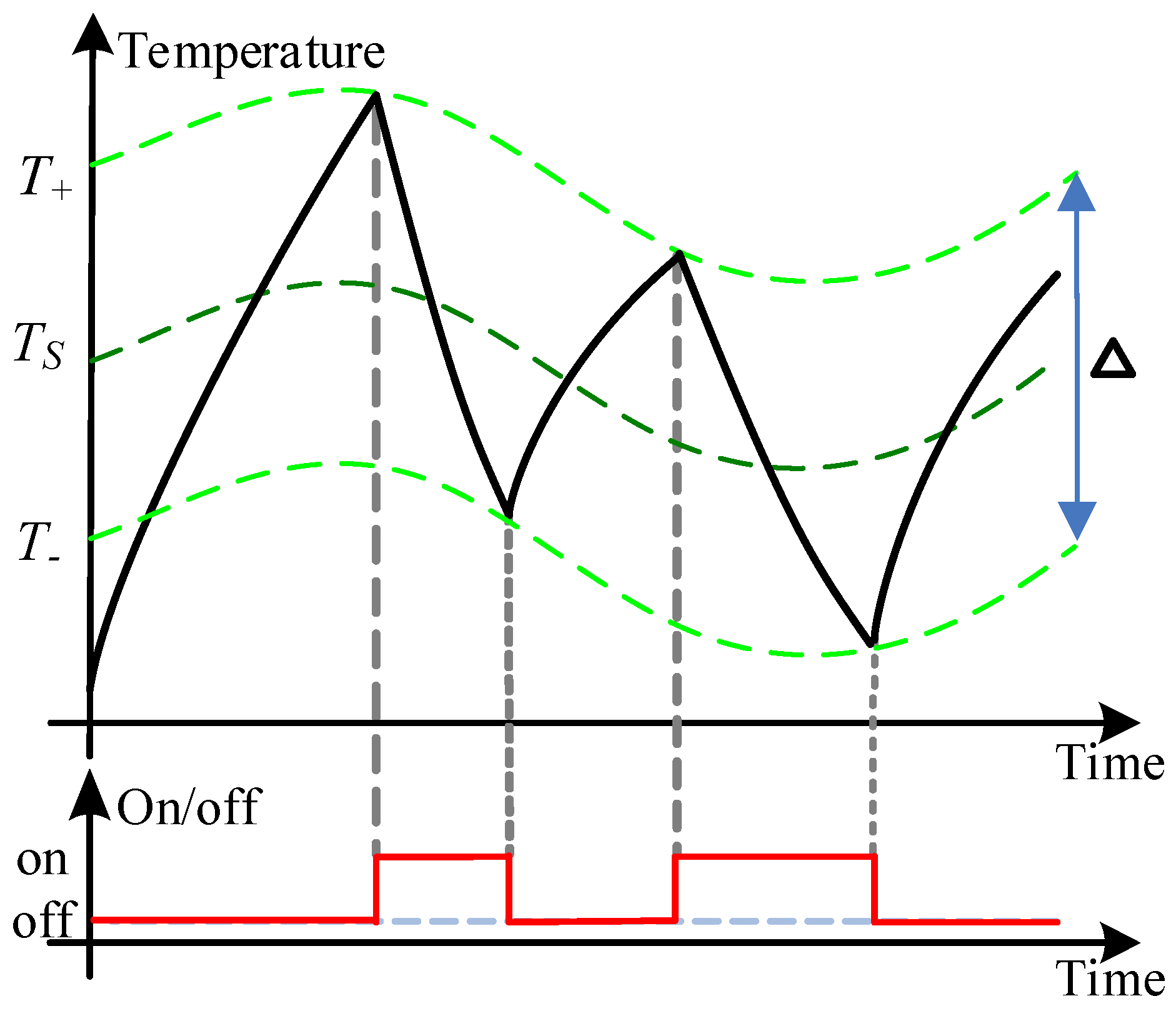
Figure 3.
System structure diagram.

Figure 4.
Fuzzy neural network structure diagram.

Figure 5.
Flow chart of the optimization algorithm.
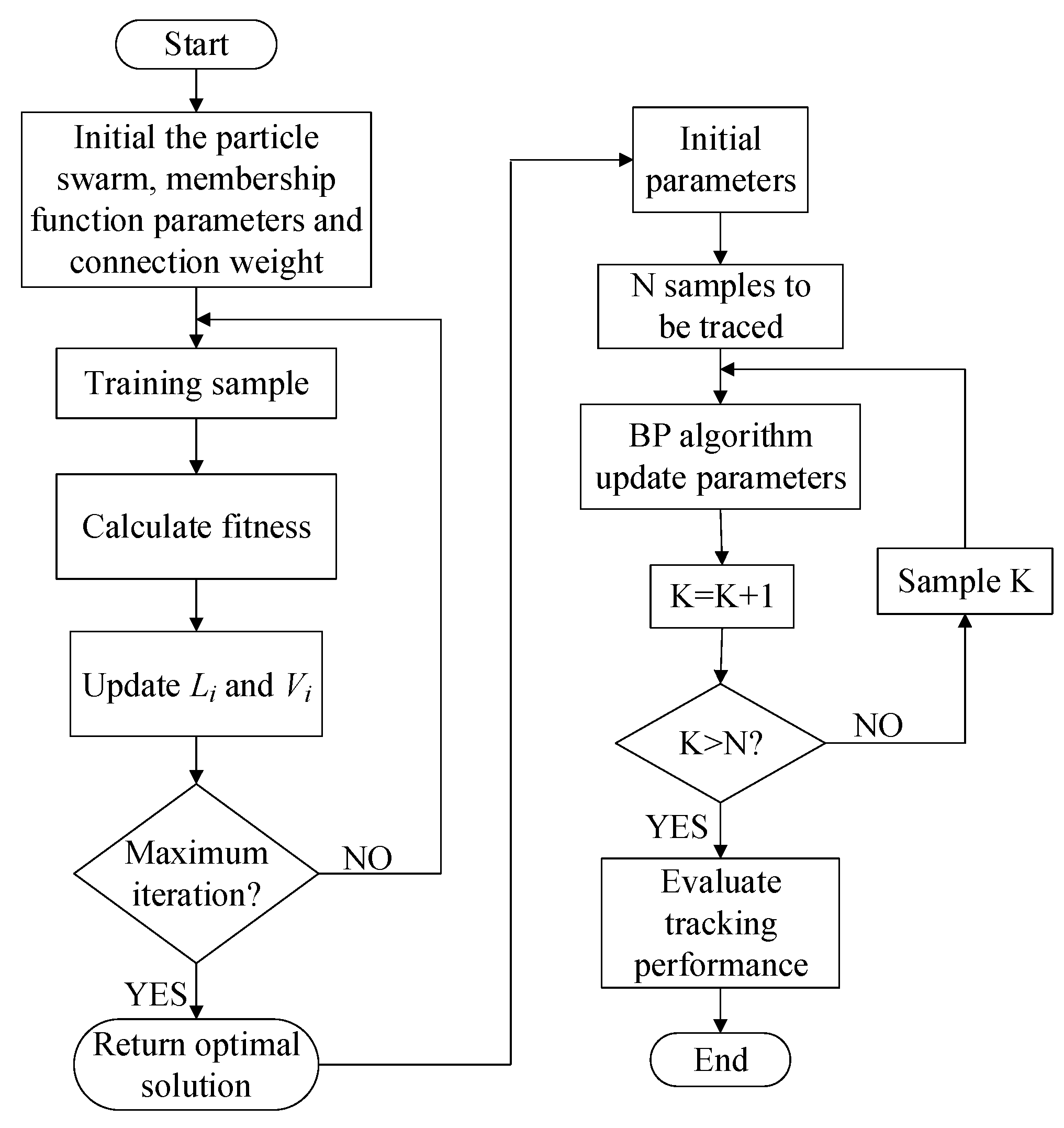
Figure 6.
The membership function of error e.

Figure 7.
The membership function of error variation .
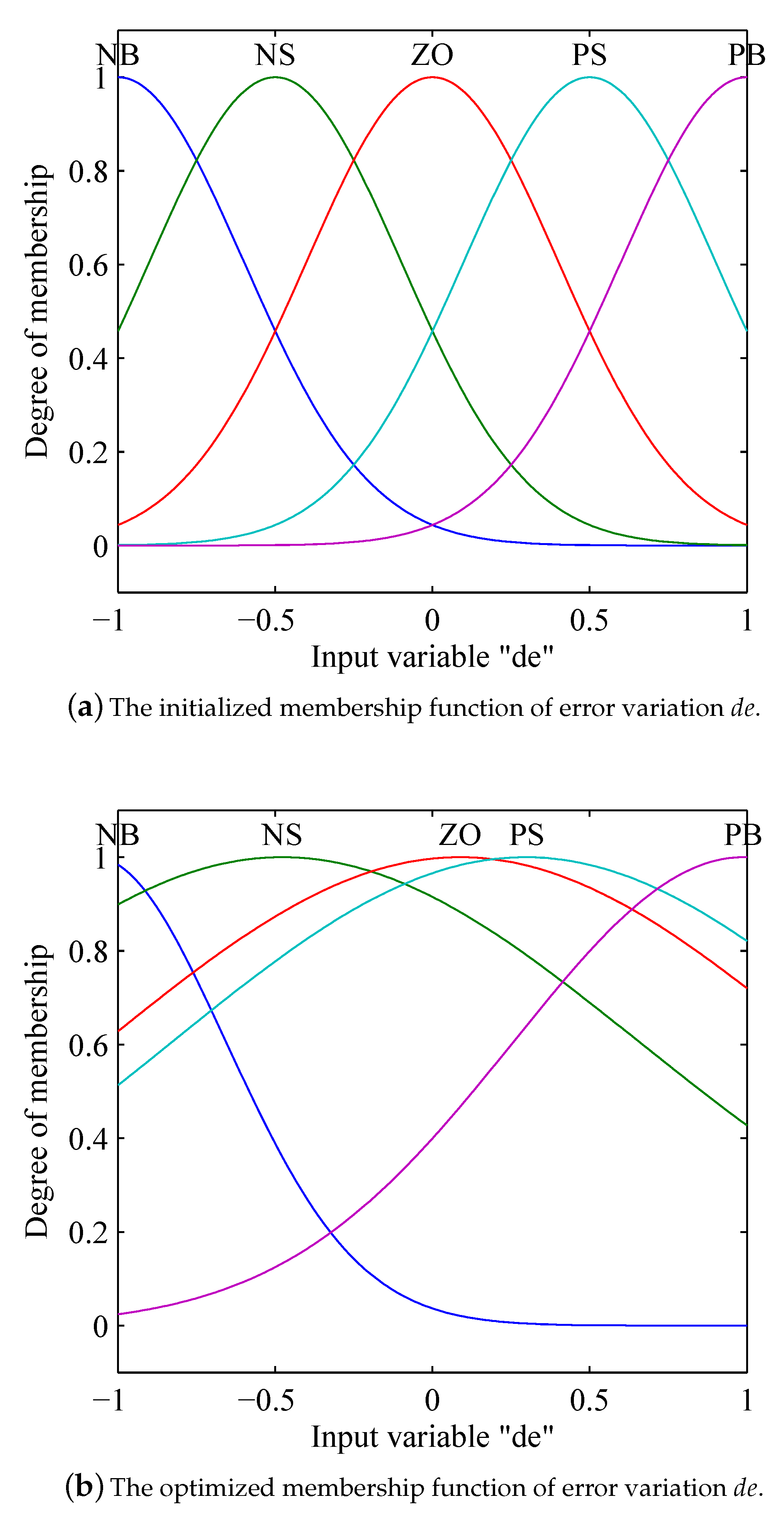
Figure 8.
Error comparisons with non-optimized and optimized parameters.
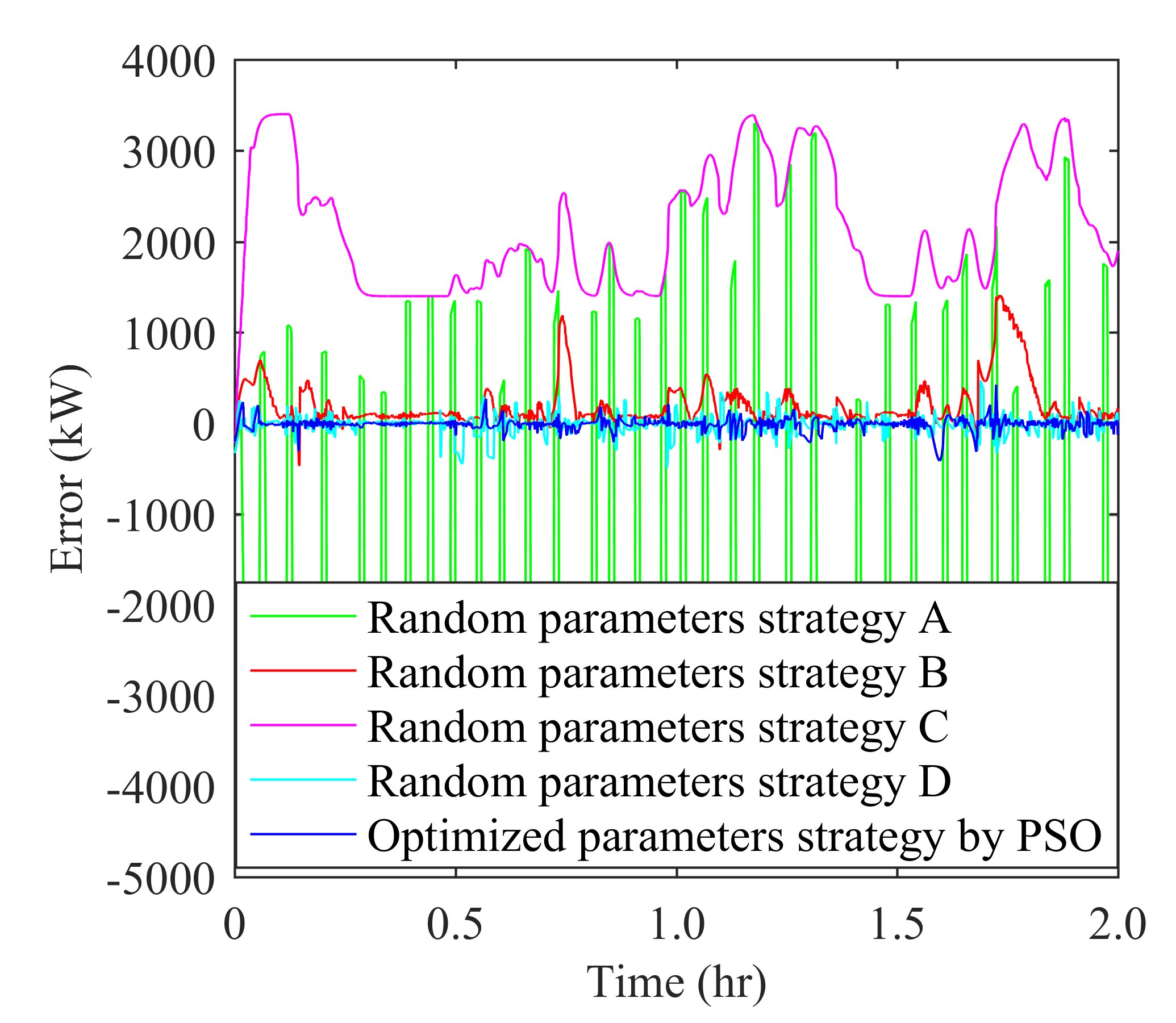
Figure 9.
Automatic generation control (AGC) signal tracking.

Figure 10.
The temperature set-point change.

Figure 11.
Error comparisons under five control strategies.

Table 1.
Comparison results.
| Control Strategies | RMSE/% | Set-Point Range/C | Average On/Off Time |
|---|---|---|---|
| On/off control [27] | 19.75 | 20 | 62 |
| On/off control with the step rule [28] | 14.22 | 20 | 45 |
| Set-point regulation [16] | 4.01 | 19.83 ∼ 21.11 | 26 |
| Set-point regulation with (,) [28] | 2.80 | 19.82 ∼ 21.02 | 15 |
| Fuzzy neural network control | 2.33 | 19.83 ∼ 21.18 | 8 |
© 2019 by the authors. Licensee MDPI, Basel, Switzerland. This article is an open access article distributed under the terms and conditions of the Creative Commons Attribution (CC BY) license (http://creativecommons.org/licenses/by/4.0/).
Share and Cite
MDPI and ACS Style
Qu, Z.; Xu, C.; Ma, K.; Jiao, Z. Fuzzy Neural Network Control of Thermostatically Controlled Loads for Demand-Side Frequency Regulation. Energies 2019, 12, 2463. https://doi.org/10.3390/en12132463
AMA Style
Qu Z, Xu C, Ma K, Jiao Z. Fuzzy Neural Network Control of Thermostatically Controlled Loads for Demand-Side Frequency Regulation. Energies. 2019; 12(13):2463. https://doi.org/10.3390/en12132463
Chicago/Turabian StyleQu, Zhengwei, Chenglin Xu, Kai Ma, and Zongxu Jiao. 2019. "Fuzzy Neural Network Control of Thermostatically Controlled Loads for Demand-Side Frequency Regulation" Energies 12, no. 13: 2463. https://doi.org/10.3390/en12132463
Note that from the first issue of 2016, this journal uses article numbers instead of page numbers. See further details here.