Short-Term Electric Power Demand Forecasting Using NSGA II-ANFIS Model

Abstract

Load forecasting is of crucial importance for smart grids and the electricity market in terms of the meeting the demand for and distribution of electrical energy. This research proposes a hybrid algorithm for improving the forecasting accuracy where a non-dominated sorting genetic algorithm II (NSGA II) is employed for selecting the input vector, where its fitness function is a multi-layer perceptron neural network (MLPNN). Thus, the output of the NSGA II is the output of the best-trained MLPNN which has the best combination of inputs. The result of NSGA II is fed to the Adaptive Neuro-Fuzzy Inference System (ANFIS) as its input and the results demonstrate an improved forecasting accuracy of the MLPNN-ANFIS compared to the MLPNN and ANFIS models. In addition, genetic algorithm (GA), particle swarm optimization (PSO), ant colony optimization (ACO), differential evolution (DE), and imperialistic competitive algorithm (ICA) are used for optimized design of the ANFIS. Electricity demand data for Bonneville, Oregon are used to test the model and among the different tested models, NSGA II-ANFIS-GA provides better accuracy. Obtained values of error indicators for one-hour-ahead demand forecasting are 107.2644, 1.5063, 65.4250, 1.0570, and 0.9940 for RMSE, RMSE%, MAE, MAPE, and R, respectively.

1. Introduction

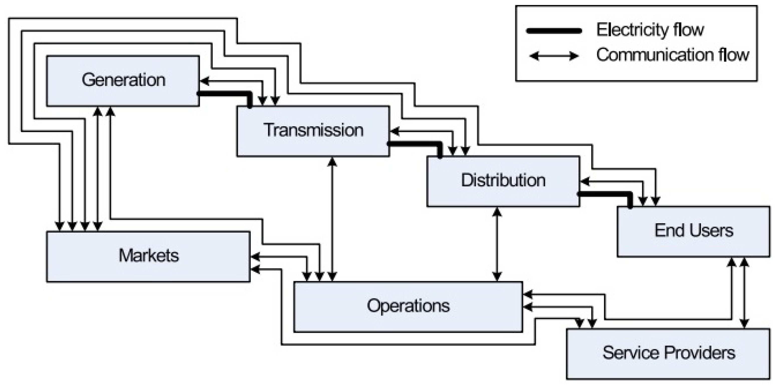
Planning electricity systems in terms of generation, transmission, and distribution relies on generation and load forecasting. In addition to economic load dispatching, unit commitment, and price forecasting which, are interests of the electricity market, electrical load forecasting is important in terms of risk reduction for the power grid. In addition, unbalanced supply/demand caused by inaccurate forecasts in traditional electricity generation systems [1] has led to integration of advanced communication technologies into traditional grids, which are known as smart girds (Figure 1). Smart grids engage the customer in the decision-making process and, in a larger view, decisions are made based on the flow and exchange of information [2]. However, there are challenges to ensure that smart grids are economically beneficial, such as closing the gap between demand and supply, and fuel resource planning. All these factors highlight the importance of accurate electrical energy demand forecasts.

Diverse techniques have been applied in demand forecasting problems such as techniques based on time series and regression analysis [3,4,5]. However, because of the non-linear nature of the problem, techniques based on artificial neural networks and Adaptive Neuro-Fuzzy Inference System (ANFIS) are more popular [6,7,8,9,10,11]. As an example, Barak and Sadegh [12] proposed a hybrid ARIMA-ANFIS model for forecasting of the annual energy consumption of Iran. ARIMA outputs were used to forecast the energy consumption, using different ANFIS structures. According to the results, the ARIMA-ANFIS model gave more accurate forecasts compared to the ARIMA and ANFIS models. As the final step, meta-heuristic algorithms were employed to increase the accuracy of the ANFIS. The research does not develop a strategy for large data sets and input selection.

In another piece of research conducted by Hooshmand et al. [13], a wavelet transform (WT) and an artificial neural network (ANN) were used for primary load forecasting where the inputs are meteorological parameters and previous values of the electric load. The ANFIS was employed to improve the forecasting results. However, the research does not introduce an approach for input selection and the capability of the evolutionary algorithms for optimizing the ANFIS has not been investigated. In another similar model, Panapakinis and Dagoumas [14] proposed a wavelet transform-ANFIS-GA-neural network model for natural gas demand forecasting. The original signal was decomposed by WT and used as ANFIS inputs. After optimizing ANFIS parameters with GA, output of ANFIS was fed into the neural network. The model does not seem to be efficient in case of multiple inputs since feature selection approach has not been developed.

A difference seasonal auto-regressive integrated moving average (diff-SARIMA), neural network, ANFIS, and DE combined method was used by Yang et al. [15] for short-term electricity demand forecasting of New South Wales in Australia. The proposed combined model presented better results than SARIMA, neural network, and ANFIS models. Parameters of the ANFIS were optimized using the DE method. Identical to the articles mentioned earlier, the research does not present a strategy for input selection. Moon et al. [16] proposed a hybrid of random forest and multi-layer perceptron for daily energy demand forecasting of a university campus. A decision tree was employed to classify the data into date, day of the week, holiday, and academic year. Furthermore, an approach was developed for considering the effect of the temperature in energy consumption and classifying the days of the week. However, the algorithm might not easily adapt to availability of the other parameters to be considered.

All the issues mentioned earlier motivated the current study to develop a forecasting strategy which: (i) can perform with any given dataset; (ii) is totally automatized; and (iii) provides a better accuracy.

Contribution

The current study aims to address solutions for data pre-processing and the input selection problem. As mentioned above, previous studies did not develop a robust model that is compatible with different datasets. The best combination of the input variables must be achieved before applying any data pre-processing or feature extraction techniques. The paper proposes a robust model which is capable of forecasting hourly electrical load demand with any given inputs. The inputs may include different combinations of previous demand values and weather parameters.

In addition, despite a combination of ANNs and ANFIS being discussed in previous research, training ANFIS was realized using a hybrid method. The proposed methodology employs meta-heuristic algorithms for ANFIS training and combines MLPNN, ANFIS, and meta-heuristics to increase the forecasting accuracy. Some research related to training ANFIS using meta-heuristics is given in [17,18,19,20].

The proposed methodology is described in Section 2 and the results are presented and discussed in Section 3. Finally, Section 4 is the conclusion of the present study.

2. Methodology

2.1. Data

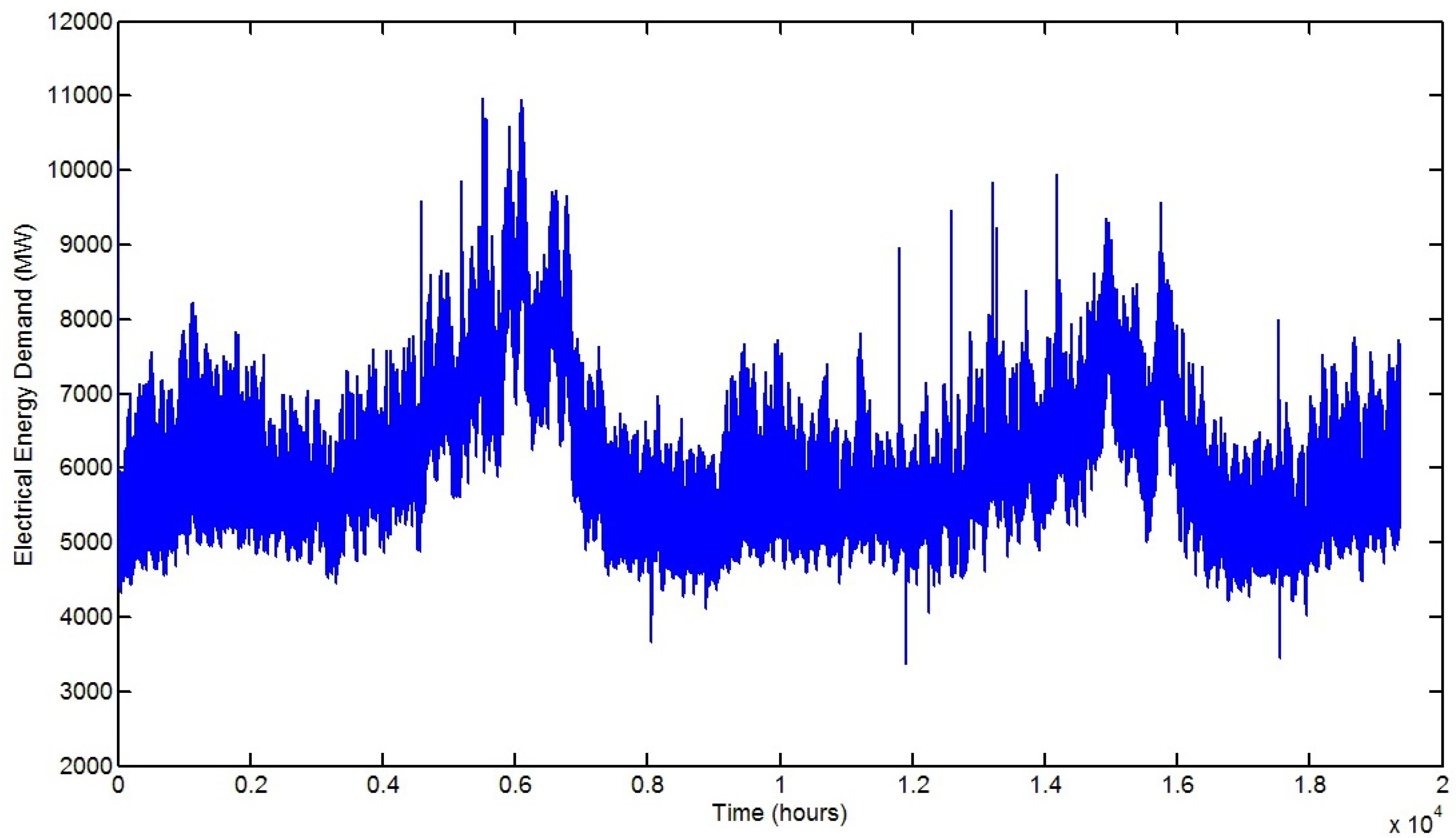
Hourly electrical power demand data for Bonneville, Oregon, USA, from 2 July 2015 to 19 September 2017 provided by the US Energy Information Administration [21] were used to test and validate the model. The original data set was a $1\times n$ matrix where n is the number of samples. After removing the matrix fields without reported values, a figure of the initial dataset was generated and presented in Figure 2.

A new data set ($13\times (n-30)$ matrix) was created where 30 is the biggest considered delay. 13 is related to the applied probable delays of 1, 2, 3, 4, 5, 6, 24, 25, 26, 27, 28, 29, and 30 for creating a dataset with 13 variables. To obtain the best combination of the variables, a new dataset was fed into the NSGAII as described in Section 2.2. Outlier detection techniques can be applied for detection and removal of outliers. An example of these techniques is given in [22].

2.2. Proposed Algorithm

The created input dataset contains ($x-1$), ($x-2$), ($x-3$), ($x-4$), ($x-5$), ($x-6$), ($x-24$), ($x-25$), ($x-26$), ($x-27$), ($x-28$), ($x-29$), ($x-30$) variables where x is the actual electrical power demand. These are the inputs of the NSGA II which can generate results with any given input dataset and find the best combination of the inputs. Thus, other delays of the electrical power demand and weather parameters (if available) can be added to the inputs.

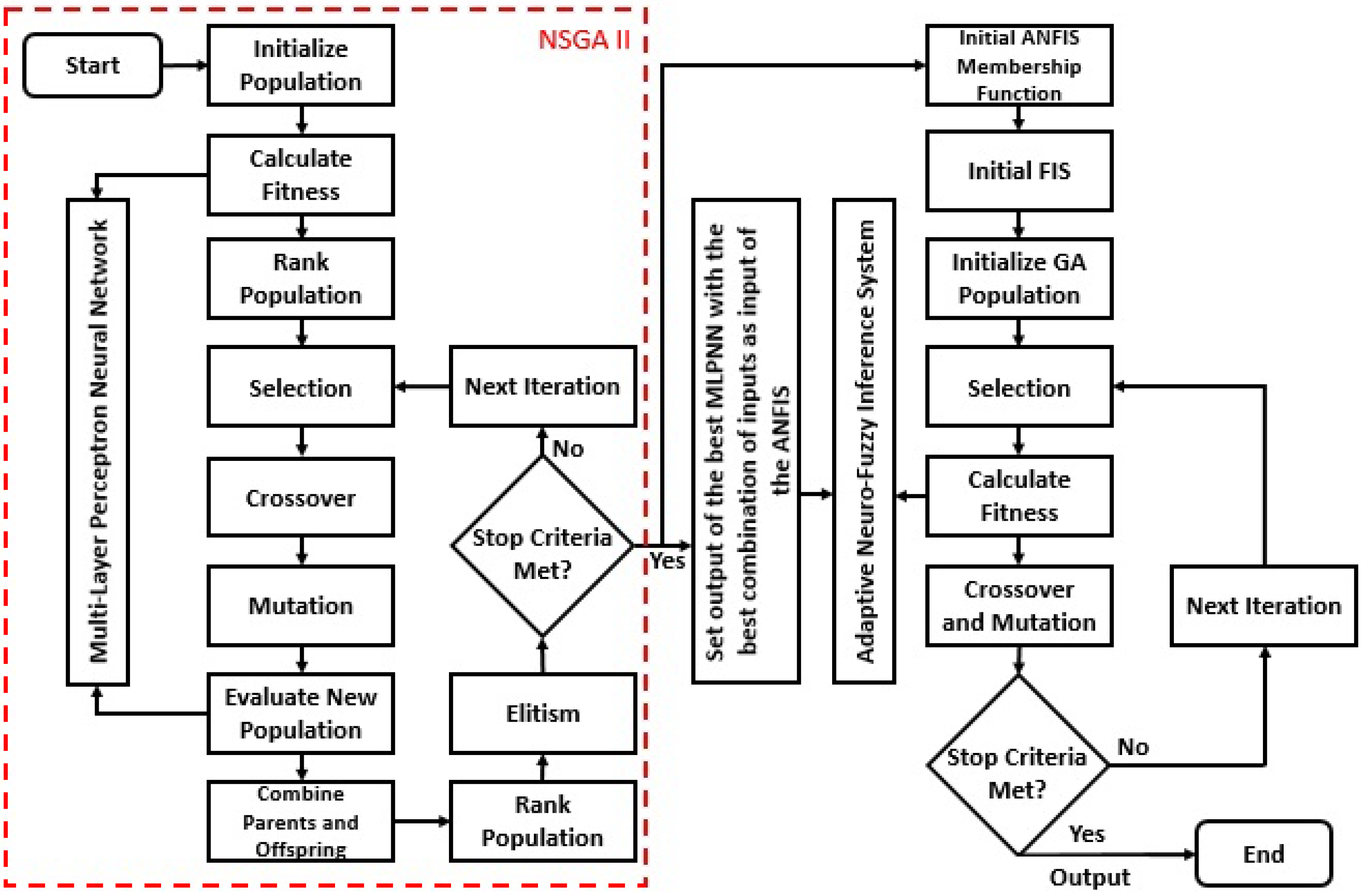
The proposed algorithm is a two-step forecasting process. In the primary forecasting step, a combination of the NSGAII and MLPNN was employed. MLPNN is the fitness function of the NSGA II to determine fitness of the input combinations in each iteration of the NSGAII. The output of the NSGAII was set to be the MLPNN with the best fitness. Therefore, the obtained MLPNN contains the best combination of the input variables among tested combinations in iterations of the NSGAII and is also the best-trained neural network.

As the second step, the obtained forecasted value from the first step was fed to the ANFIS. The result of this step is the final forecasted value of the electrical energy demand. Training of the ANFIS was realized using different algorithms, namely hybrid algorithm (combination of the backpropagation and least-square error), ACO, DE, GA, ICA, and PSO. Among applied algorithms for ANFIS training, GA demonstrated better performance in terms of the lower values of error indicators. The overall proposed approach is presented in Figure 3.

2.2.1. NSGA II

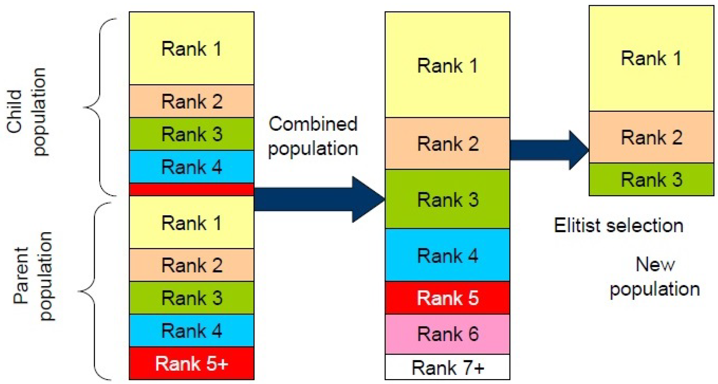
NSGA II [23] is an elitist multi-objective optimization algorithm that initializes by a random population and assigns a fitness value for each member of the population. After generating the offspring using crossover and mutation operators, a binary selection operator, based on fitness and crowding distance, is applied to the parent and offspring population for elitist selection. Crowding distance defines the distance of an individual to its neighbors and large crowding distance results in higher diversity, calculating the crowding distance begins by assigning distance to zero for each individual. Next, individuals are sorted based on objective function. After assigning infinite value to the boundaries ($I\left(d_1\right)=\infty ,I\left(d_n\right)=\infty )$, crowding distance of the mth objective function of the kth individual in front $F_i$ for $k=2$ to $(n-1)$ is calculated by Equation (1).

$$I\left(d_k\right)=I\left(d_k\right)=\frac{I(k+1)·m-I(k-1)·m}{f_m^{max}-f_m^{min}}$$

(1)

The algorithm preserves the best individuals from parent and offspring and continues until the stopping criteria is met. The elitism process is shown in Figure 4.

2.2.2. MLPNN

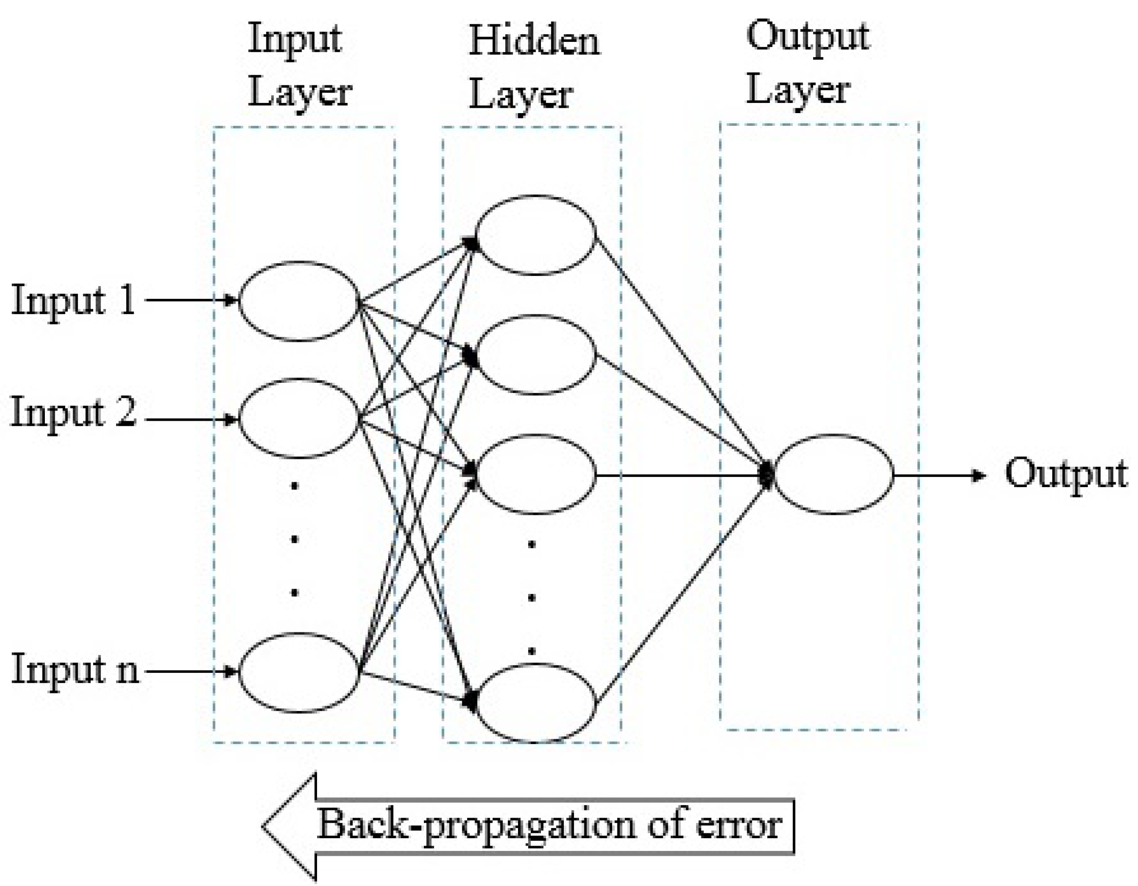
Multi-layer perceptron neural network is a powerful tool for solving non-linear problems. It consists of an input layer, one or more hidden layers, and an output layer. Each layer contains artificial neurons and the neurons between layers are connected with an adaptable weight. The output of each neuron in each layer is multiplied by the adaptable weight and after passing through a transfer function becomes the input to the next-level neurons. In this research, tuning the weights, which is called the learning process, is realized by a backpropagation algorithm, namely the Levenberg-Marquardt algorithm. The structure of an MLPNN is shown in Figure 5.

2.2.3. ANFIS

ANFIS was introduced by Jang [24] and is an artificial intelligence model that benefits from advantages of both fuzzy systems and ANNs. In this model, fuzzy inference systems (FIS) are determined by if-then rules and membership functions (MFs) where tuning the MFs are realized by ANNs. The three main types of FISs are the Takagi-Sugeno-Kang (TSK), Mamdani, and Tsumoto [25]. In this research, TSK FIS model was employed, which is more powerful at handling non-linear input-output relationships [26]. TSK uses the pattern of input and output data to create if-then rules. If-then rules for TSK model in a 2-input system is given in Equation (2).

$$\begin{array}{c}Ifx=A_{1}andy=B_1\Rightarrow f=p_{1}x+q_{1}x+r_1\\ Ifx=A_{2}andy=B_2\Rightarrow f=p_{2}x+q_{2}x+r_2\end{array}$$

(2)

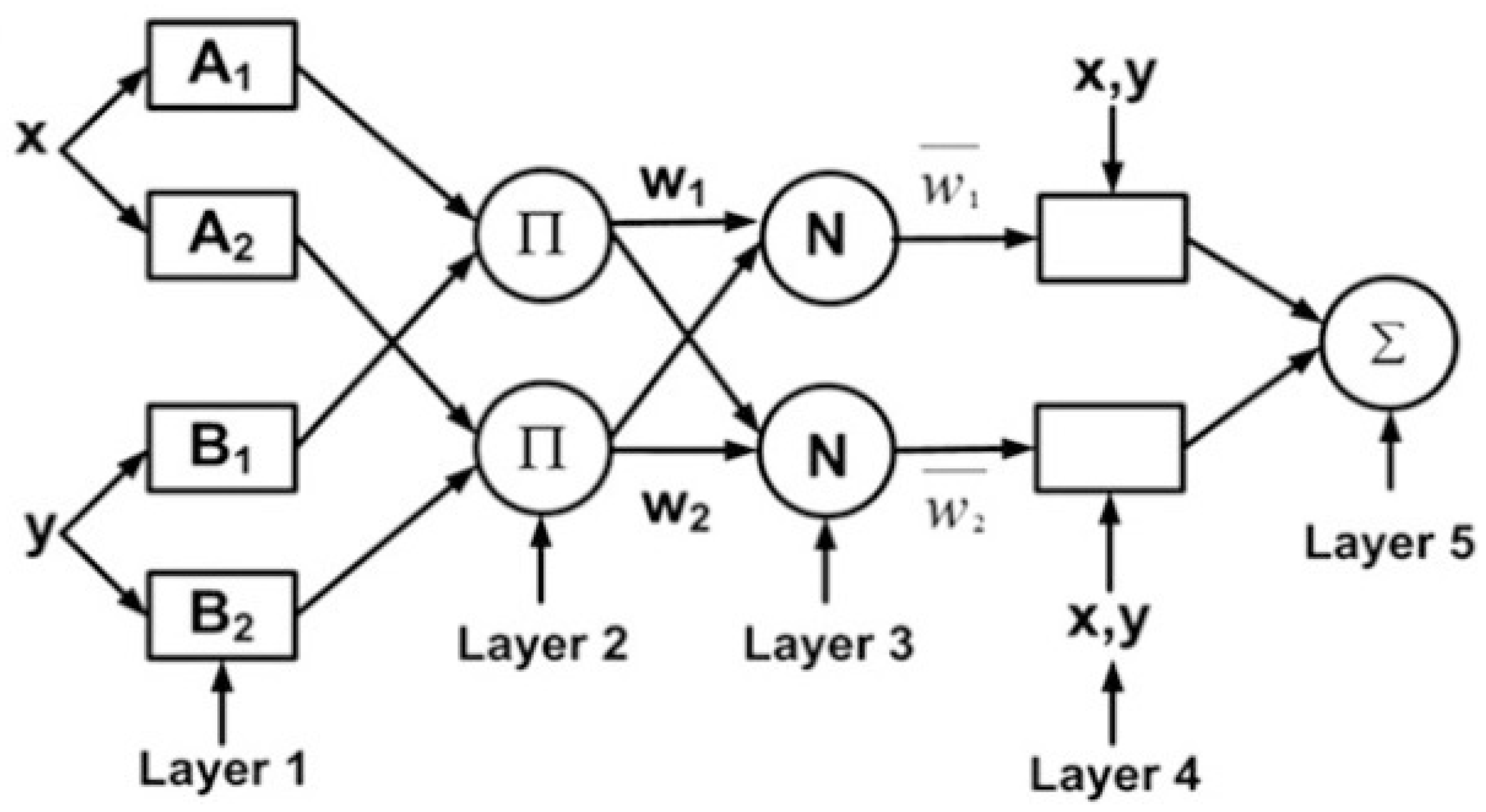
where $A_1$, $B_1$ and $A_2$, $B_2$ are the MFs related to input x and input y respectively and $p_1$, $q_1$, $r_1$, $p_2$, $q_2$, $r_2$ are linear parameters of part-Then in TSK. Figure 6 shows the structure of a typical ANFIS model which contains 5 layers.

The fuzzification process is realized in the first layer. In this layer, nodes are square nodes with function presented in Equation (3).

$$O_i^1=\mu A_i\left(x\right)$$

(3)

where i is the ith node in the layer, $A_i$ is linguistic value of the node. As the membership function, a Gaussian membership function was employed (Equation (4)).

$$\mu A_i\left(x\right)=exp\left[-{(\frac{x-c_i}{2a_i})}^2\right]$$

(4)

where $a_i$ and $c_i$ are the parameters that define shape of the membership function. These parameters are tuned during the learning process. Layer 2 contains circle nodes that multiply the input signals and their output is the product of this multiplication which stands for firing strength of each rule as given in Equation (5).

$${\omega }_i=\mu A_i\left(x\right)\times \mu B_i\left(y\right),i=1,2.$$

(5)

In layer 3, node i calculates the ratio of ith rule firing strength in respect to sum of all rules firing strength which, is a normalization process. Similar to layer 2, nodes are fixed in layer 3. Next, adaptive nodes in layer 4 calculate values of the rule of the consequent part and finally, layer 5 sums all outputs of layer 4 and contains only one node [27]. Mathematical description of layer 3, layer 4 and layer 5 are given in Equations (6)–(8) respectively.

$${\overline{\omega }}_i=\frac{{\omega }_i}{{\omega }_1+{\omega }_2},i=1,2.$$

(6)

$$O_i^4={\overline{\omega }}_i{f}_i={\overline{\omega }}_i(p_{i}x+q_{i}y+r_i).$$

(7)

$$O_i^5=\sum _i{\overline{\omega }}_i{f}_i=\frac{{\sum }_i{\omega }_i{f}_i}{{\sum }_i{\omega }_i}.$$

(8)

ANFIS is trained using input-output data pairs. As seen in the ANFIS architecture and equations describing each layer, parameters in layer 1 and layer 4 can be tuned. This process defines the shape of the MFs (tuning of $a_i$ and $c_i$) and specifies the fuzzy rules (tuning of $p_i$, $q_i$ and $r_i$). Tuning of these parameters is realized according to an error criterion. Backpropagation algorithm can be employed for training ANFIS; however, due to slow convergence rate of the backpropagation algorithm and its tendency to be trapped in local minima, it is used combined with the least-square estimator. This combination is called the hybrid method and because of reduction of the dimensional search space, provides a faster convergence rate [28].

2.2.4. Genetic Algorithm (GA)

A genetic algorithm is a meta-heuristic algorithm based on natural selection. A continuous GA was used for this research, which consists of mutation, crossover, and selection. To distribute the initial population in solution space, the initial population is generated randomly. The solutions in each iteration are evolved until the stopping criteria is met.

3. Results and Discussion

3.1. Primary Forecasting Step

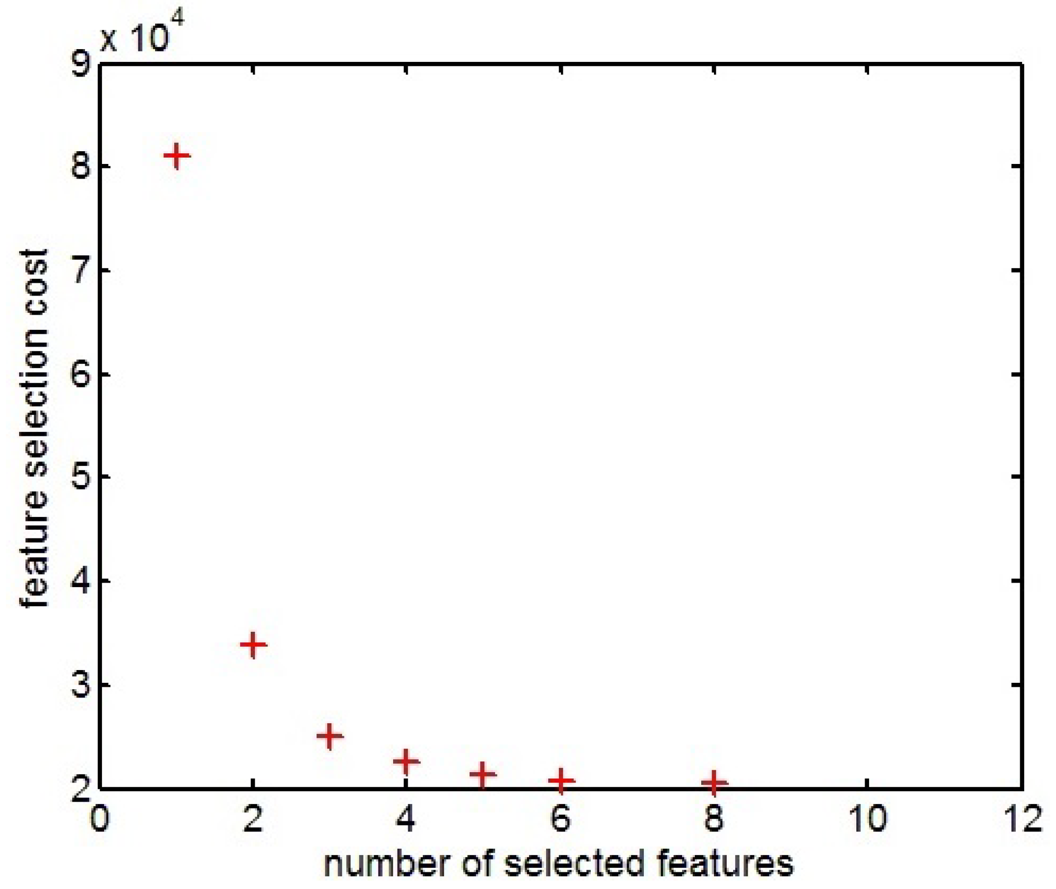
As the primary forecasting step, the created data matrix with 13 variables was fed into the NSGAII algorithm. The employed fitness function is an MLPNN with one hidden layer whose hidden layer size and transfer functions are 7, tansig, and tansig, respectively. Different combinations of the 13 variables (input vectors) were generated, and their fitness values were evaluated by the NSGAII in each iteration. Non-dominated solutions are the outputs of this step. Each output is a MLPNN, which contains the best non-dominated input vector as its input. The Pareto front of the NSGAII related to the generated non-dominant solutions is shown in Figure 7.

To demonstrate the importance of the feature selection, forecasting results of the best input vector generated by NSGAII was compared to the 13 variables 1 variable (x − 1) input vectors, using MLPNN as the forecasting model. The results are presented in

Table 1. Forecasting results for different input sets using MLPNN.

Input Set	$\mathbf{RMSE}\left(\mathbf{MW}\right)$	$\mathbf{RMSE}(\%)$	MAE (MW)	$\mathbf{MAPE}(\%)$	R
1 input	301.7724	3.8788	195.0414	3.1479	0.9523
Selected inputs by NSGA II	136.1048	1.7409	68.3688	1.0950	0.9904
All Inputs	160.5449	2.0636	69.4196	1.1029	0.9866

. Explanation of the employed error indicators can be found in Appendix A.

As seen in Table 1, using selected input vector generated by the NSGA II results in better forecasting accuracy. Furthermore, to compare the forecasting accuracy of the MLPNN and ANFIS models, the selected input vector was used as the input of the ANFIS models with different training algorithms. The results are given in

Table 2. Forecasting results for each model.

Model	$\mathbf{RMSE}\left(\mathbf{MW}\right)$	$\mathbf{RMSE}(\%)$	MAE (MW)	$\mathbf{MAPE}(\%)$	R
ANFIS-ACOR	207.2688	2.8755	98.9818	1.5777	0.9775
ANFIS-Hybrid	194.6117	2.4017	86.8079	1.3838	0.9803
ANFIS-DE	202.3010	2.1925	100.7624	1.6181	0.9795
ANFIS-GA	190.1248	2.1810	97.4025	1.5438	0.9820
ANFIS-ICA	288.7683	3.8939	208.4114	3.3892	0.9577
ANFIS-PSO	195.7518	2.1215	83.5948	1.3360	0.9805

.

Comparing Table 1 to Table 2 it can be observed that using selected input vector, MLPNN model has a better forecasting accuracy compared to the ANFIS model. In addition, among tested ANFIS training algorithms, GA demonstrates better performance. Response surface of output versus input 1 and input 2 related to hybrid learning algorithm and GA learning algorithm (meta-heuristic with the best performance) are given in Figure 8 where input 1 and input 2 are (x − 1) and (x − 2) respectively.

3.2. Final Forecasting Step

In the primary forecasting step, variables were selected by the NSGAII and an output was generated which is an MLPNN with selected input vector. As the final step, output of the MLPNN was fed into the created ANFIS models with different training algorithms, to evaluate the ability of the ANFIS to increase the forecasting results of the MLPNN model. The results are given in

Table 3. Forecasting results for each model.

Model	$\mathbf{RMSE}\left(\mathbf{MW}\right)$	$\mathbf{RMSE}(\%)$	MAE (MW)	$\mathbf{MAPE}(\%)$	R
MLPNN-ANFIS-ACOR	175.1901	1.8987	69.1994	1.1033	0.9842
MLPNN-ANFIS-Hybrid	142.6229	1.8243	66.5694	1.0603	0.9896
MLPNN-ANFIS-DE	158.2172	1.9138	68.2244	1.0967	0.9869
MLPNN-ANFIS-GA	107.2644	1.5063	65.4250	1.0570	0.9940
MLPNN-ANFIS-ICA	121.7895	1.5229	65.5095	1.0639	0.9922
MLPNN-ANFIS-PSO	148.1894	2.0559	66.8190	1.0641	0.9886

.

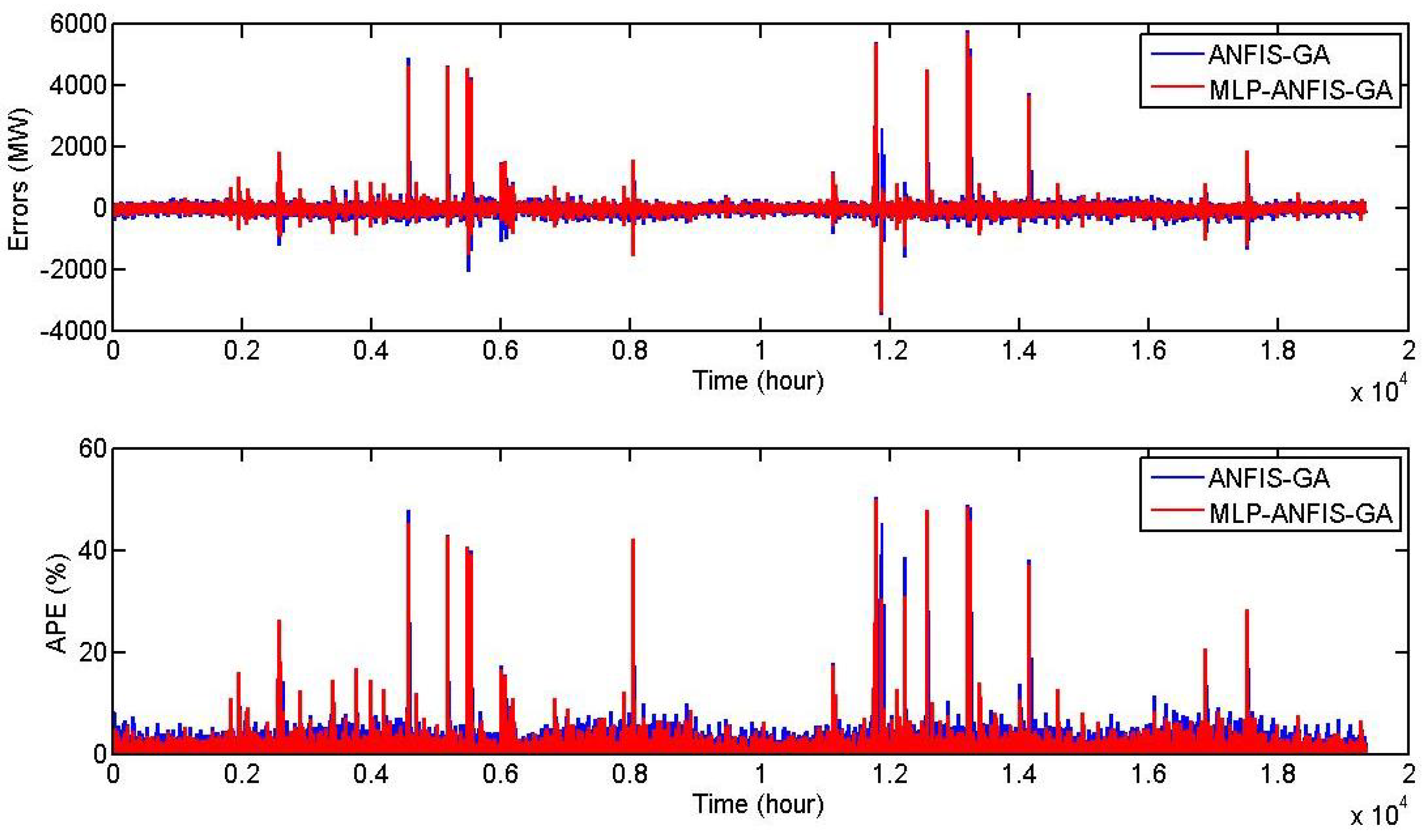
As seen in Table 3, the combination of the MLPNN and ANFIS models improves the forecasting accuracy and MLPNN-ANFIS models and demonstrates lower error rates compared to the MLPNN and ANFIS models. Furthermore, all error indicators of RMSE, MAE, MAPE, and R related to MLPNN-ANFIS-GA model are lower than MLPNN-ANFIS-GA model. Thus, GA has a better performance in ANFIS training compared to the hybrid method. Figure 9 presents the errors and absolute percentage error (APE) for ANFIS-GA and MLPNN-ANFIS-GA models to better demonstrate the increased forecasting accuracy using a combination of MLPNN and ANFIS.

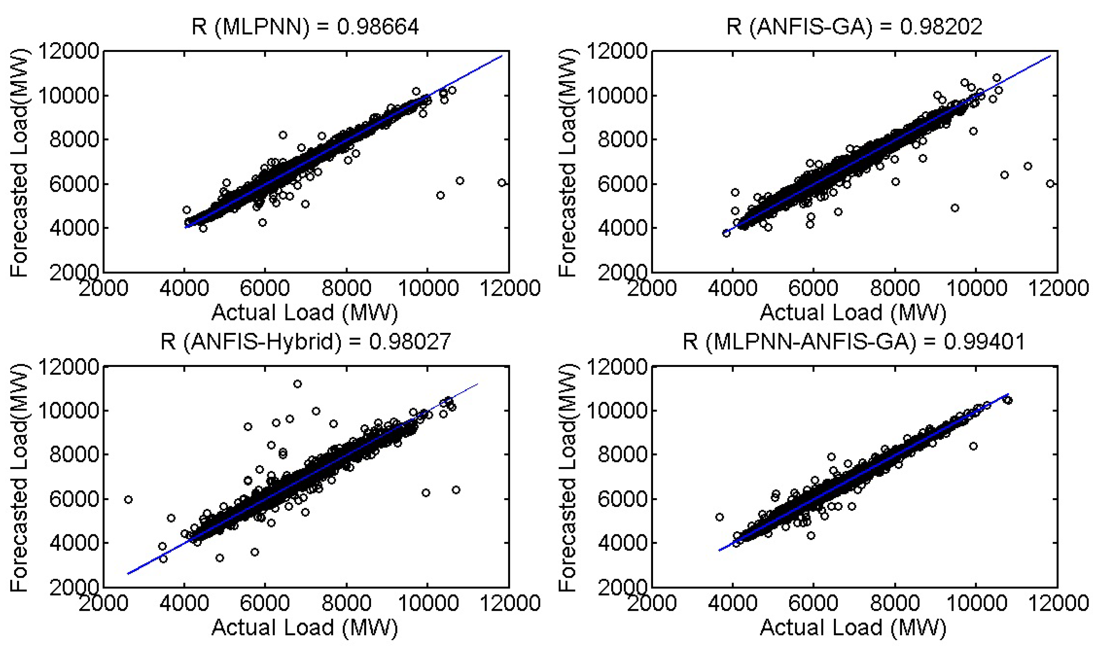
For the purposes of better illustrating the accuracy of the tested models, error indication of the correlation coefficient for MLPNN, ANFIS-Hybrid, ANFIS-GA, and MLPNN-ANFIS-GA models are presented in Figure 10 while error indicators for these models are presented in

Table 4. Error indicators for MLPNN, ANFIS-Hybrid, ANFIS-GA, and MLPNN-ANFIS-GA models using the selected input vector by NSGAII.

Model	$\mathbf{RMSE}\left(\mathbf{MW}\right)$	$\mathbf{RMSE}(\%)$	MAE (MW)	$\mathbf{MAPE}(\%)$	R
MLPNN	136.1048	1.7409	68.3688	1.0950	0.9904
ANFIS-Hybrid	194.6117	2.4017	86.8079	1.3838	0.9803
ANFIS-GA	190.1248	2.1810	97.4025	1.5438	0.9820
MLPNN-ANFIS-GA	107.2644	1.5063	65.4250	1.0570	0.9940

.

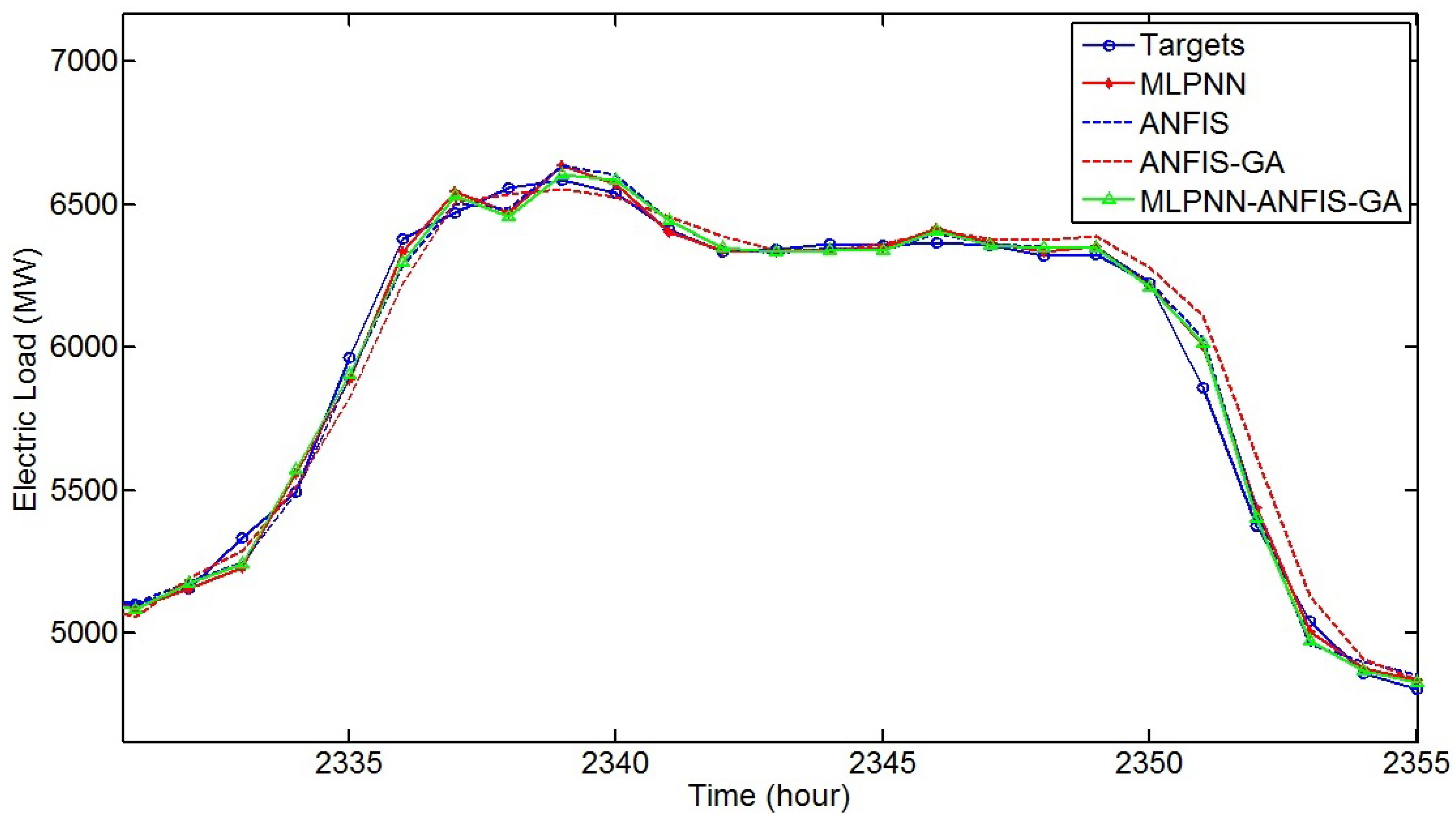
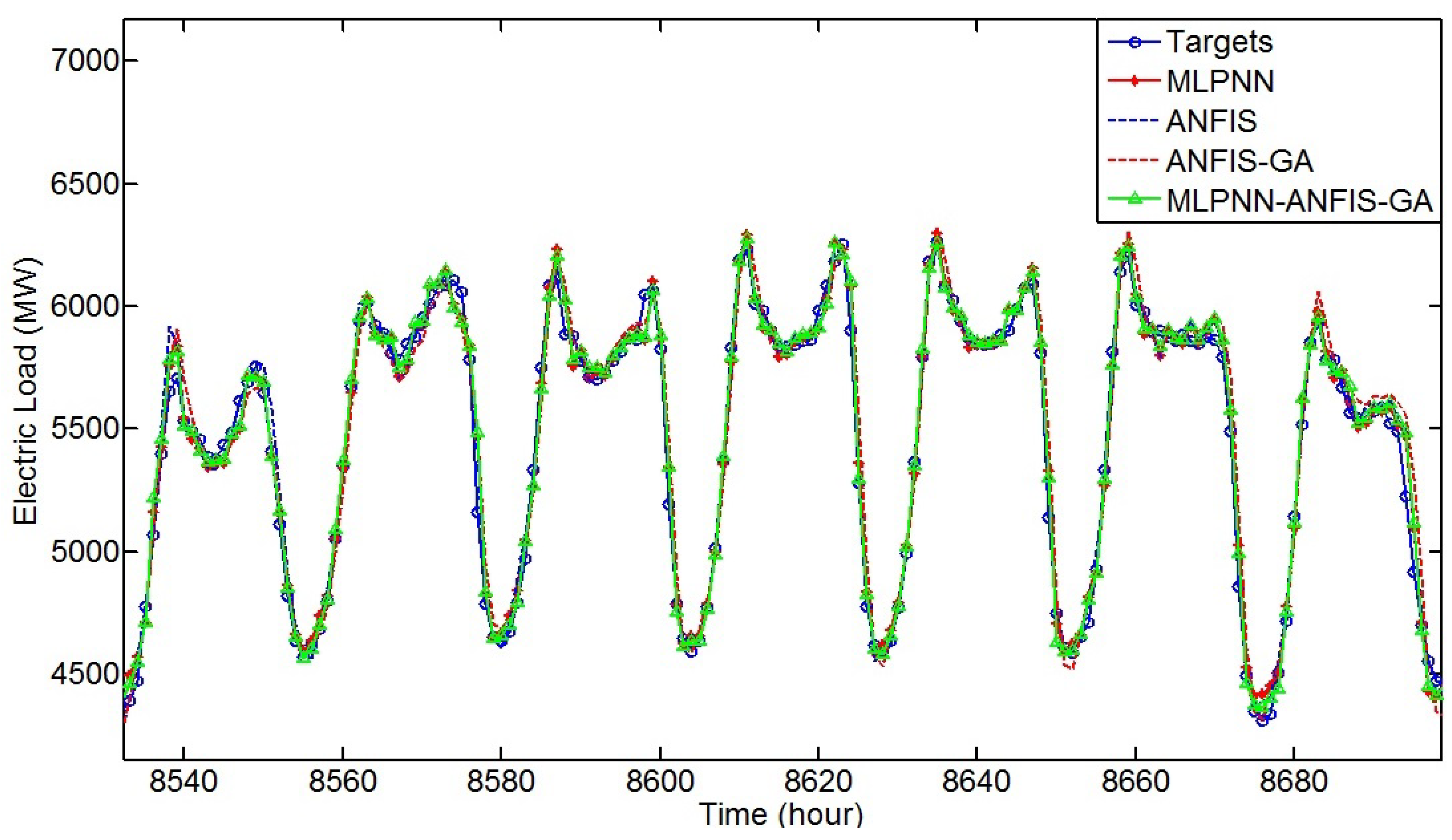
As seen, the MLPNN-ANFIS-GA model provides the best correlation coefficient and lower error rates in terms of the RMSE, MAE, and MAPE among the tested models. The targets (actual load) and the final forecasting results for a one-day region and a one-week region are presented in Figure 11 and Figure 12 respectively.

4. Conclusions

In all forecasting problems, input parameter selection is of great importance. The developed methodology in the current research proposes a solution to the trial-and-error approach employed by previous research in a demand forecasting field. The developed approach is compatible with any given dataset and can perform in cases of addition or removal of input variables. Assigning a multi-layer perceptron neural network as the output of NSGAII makes it possible to realize secondary processes automatically which, in the case of the current research, is using the ANFIS model to improve forecasting capability of the MLPNN.

Regarding processing time and computational complexity, since the most complex process is finding the input vector, once inputs are selected and the output of the NSGAII is generated, the algorithm can be used for online applications. It will be necessary to run the primary forecast part of the algorithm just in case of availability of new parameters, which can increase the forecasting accuracy.

According to the obtained results, while MLPNN has a better forecasting accuracy compared to the ANFIS, the combination of these two models reduces all forecasting error indicators. In addition, meta-heuristic algorithms are found to be suitable for training of the ANFIS. GA demonstrated better performance in terms of ANFIS training compared to the hybrid method. Among all tested models, the MLPNN-ANFIS-GA model presented lower error rates in terms of the RMSE, MAE, MAPE, and R.

References

- Hassan, S.; Khosravi, A.; Jaafar, J.; Khanesar, M.A. A systematic design of interval type-2 fuzzy logic system using extreme learning machine for electricity load demand forecasting. Int. J. Electr. Power Energy Syst. 2016, 82, 1–10. [Google Scholar] [CrossRef]
- Ahmad, A.; Javaid, N.; Mateen, A.; Awais, M.; Khan, Z.A. Short-Term Load Forecasting in Smart Grids: An Intelligent Modular Approach. Energies 2019, 12, 164. [Google Scholar] [CrossRef]
- Javed, F.; Arshad, N.; Wallin, F.; Vassileva, I.; Dahlquist, E. Forecasting for demand response in smart grids: An analysis on use of anthropologic and structural data and short term multiple loads forecasting. Appl. Energy 2012, 96, 150–160. [Google Scholar] [CrossRef]
- Tascikaraoglu, A.; Sanandaji, B.M. Short-term residential electric load forecasting: A compressive spatio-temporal approach. Energy Build. 2016, 111, 380–392. [Google Scholar] [CrossRef]
- Mori, H.; Kosemura, N. Optimal regression tree based rule discovery for short-term load forecasting. In Proceedings of the 2001 IEEE Power Engineering Society Winter Meeting, Conference Proceedings (Cat. No.01CH37194), Columbus, OH, USA, 28 January–1 February 2001; Volume 2, pp. 421–426. [Google Scholar] [CrossRef]
- Hippert, H.S.; Pedreira, C.E.; Souza, R.C. Neural networks for short-term load forecasting: A review and evaluation. IEEE Trans. Power Syst. 2001, 16, 44–55. [Google Scholar] [CrossRef]
- Rodrigues, F.; Cardeira, C.; Calado, J.M.F. The Daily and Hourly Energy Consumption and Load Forecasting Using Artificial Neural Network Method: A Case Study Using a Set of 93 Households in Portugal. Energy Procedia 2014, 62, 220–229. [Google Scholar] [CrossRef]
- Beccali, M.; Cellura, M.; Brano, V.L.; Marvuglia, A. Short-term prediction of household electricity consumption: Assessing weather sensitivity in a Mediterranean area. Renew. Sustain. Energy Rev. 2008, 12, 2040–2065. [Google Scholar] [CrossRef]
- Jadidi, A.; Menezes, R.; de Souza, N.; de Castro Lima, A.C. A hybrid GA–MLPNN Model for one-hour-ahead forecasting of the global horizontal irradiance in Elizabeth City, North Carolina. Energies 2018, 11, 2641. [Google Scholar] [CrossRef]
- Saleh, A.E.; Moustafa, M.S.; Abo-Al-Ez, K.M.; Abdullah, A.A. A hybrid neuro-fuzzy power prediction system for wind energy generation. Int. J. Electr. Power Energy Syst. 2016, 74, 384–395. [Google Scholar] [CrossRef]
- Nikolovski, S.; Baghaee, H.R.; Mlakic, D. ANFIS-Based Peak Power Shaving/Curtailment in Microgrids Including PV Units and BESSs. Energies 2018, 11, 2953. [Google Scholar] [CrossRef]
- Barak, S.; Sadegh, S.S. Forecasting energy consumption using ensemble ARIMA–ANFIS hybrid algorithm. Int. J. Electr. Power Energy Syst. 2016, 82, 92–104. [Google Scholar] [CrossRef]
- Hooshmand, R.A.; Amooshahi, H.; Parastegari, M. A hybrid intelligent algorithm based short-term load forecasting approach. Int. J. Electr. Power Energy Syst. 2013, 45, 313–324. [Google Scholar] [CrossRef]
- Panapakidis, I.P.; Dagoumas, A.S. Day-ahead natural gas demand forecasting based on the combination of wavelet transform and ANFIS/genetic algorithm/neural network model. Energy 2017, 118, 231–245. [Google Scholar] [CrossRef]
- Yang, Y.; Chen, Y.; Wang, Y.; Li, C.; Li, L. Modelling a combined method based on ANFIS and neural network improved by DE algorithm: A case study for short-term electricity demand forecasting. Appl. Soft Comput. 2016, 49, 663–675. [Google Scholar] [CrossRef]
- Moon, J.; Kim, Y.; Son, M.; Hwang, E. Hybrid Short-Term Load Forecasting Scheme Using Random Forest and Multilayer Perceptron. Energies 2018, 11, 3283. [Google Scholar] [CrossRef]
- Bakyani, A.E.; Sahebi, H.; Ghiasi, M.M.; Mirjordavi, N.; Esmaeilzadeh, F.; Lee, M.; Bahadori, A. Prediction of CO2–oil molecular diffusion using adaptive neuro-fuzzy inference system and particle swarm optimization technique. Fuel 2016, 181, 178–187. [Google Scholar] [CrossRef]
- Al-Dunainawi, Y.; Abbod, M.F.; Jizany, A. A new MIMO ANFIS-PSO based NARMA-L2 controller for nonlinear dynamic systems. Eng. Appl. Artif. Intell. 2017, 62, 265–275. [Google Scholar] [CrossRef]
- Sohrabpoor, H. Analysis of laser powder deposition parameters: ANFIS modeling and ICA optimization. Optik 2016, 127, 4031–4038. [Google Scholar] [CrossRef]
- Khosravi, A.; Nunes, R.; Assad, M.; Machado, L. Comparison of artificial intelligence methods in estimation of daily global solar radiation. J. Clean. Prod. 2018, 194, 342–358. [Google Scholar] [CrossRef]
- U.S. Energy Information Adminstration (EIA) Home Page. Available online: https://www.eia.gov/ (accessed on 17 December 2017).
- Ester, M.; Kriegel, H.P.; Sander, J.; Xu, X. A Density-Based Algorithm for Discovering Clusters in Large Spatial Databases with Noise. In Proceedings of the Second International Conference on Knowledge Discovery and Data Mining (KDD-96), Portland, OR, USA, 2–4 August 1996; pp. 226–231. [Google Scholar]
- Deb, K.; Pratap, A.; Agarwal, S.; Meyarivan, T. A fast and elitist multiobjective genetic algorithm: NSGA-II. IEEE Trans. Evol. Comput. 2002, 6, 182–197. [Google Scholar] [CrossRef]
- Jang, J.R. ANFIS: Adaptive-network-based fuzzy inference system. IEEE Trans. Syst. Man Cybern. 1993, 23, 665–685. [Google Scholar] [CrossRef]
- Yaseen, Z.M.; Ebtehaj, I.; Bonakdari, H.; Deo, R.C.; Mehr, A.D.; Mohtar, W.H.M.W.; Diop, L.; El-Shafie, A.; Singh, V.P. Novel approach for streamflow forecasting using a hybrid ANFIS-FFA model. J. Hydrol. 2017, 554, 263–276. [Google Scholar] [CrossRef]
- Karkevandi-Talkhooncheh, A.; Hajirezaie, S.; Hemmati-Sarapardeh, A.; Husein, M.M.; Karan, K.; Sharifi, M. Application of adaptive neuro fuzzy interface system optimized with evolutionary algorithms for modeling CO2-crude oil minimum miscibility pressure. Fuel 2017, 205, 34–45. [Google Scholar] [CrossRef]
- Mlakić, D.; Baghaee, H.R.; Nikolovski, S. A Novel ANFIS-based Islanding Detection for Inverter–Interfaced Microgrids. IEEE Trans. Smart Grid 2018. [Google Scholar] [CrossRef]
- Nayak, P.; Sudheer, K.; Rangan, D.; Ramasastri, K. A neuro-fuzzy computing technique for modeling hydrological time series. J. Hydrol. 2004, 291, 52–66. [Google Scholar] [CrossRef]
Figure 1.
Conceptual diagram of smart grid [2].
Figure 2.
Electrical power demand data for Bonneville, Oregon, USA, from 2 July 2015 to 19 September 2017.