Admittance Reshaping Control Methods to Mitigate the Interactions between Inverters and Grid


1
School of Automation, Guangdong University of Technology, Guangzhou 510006, China
2
College of Electrical and Information Engineering, Hunan University, Changsha 410082, China
3
Guangzhou Power Supply Co., Ltd., Guangzhou 510620, China
*
Author to whom correspondence should be addressed.
Energies 2019, 12(13), 2457; https://doi.org/10.3390/en12132457
Submission received: 20 May 2019
/
Revised: 17 June 2019
/
Accepted: 19 June 2019
/
Published: 26 June 2019
(This article belongs to the Special Issue Power Electronics and Power Quality 2019)
Abstract
:With the increasing impedance coupling between inverters and grid caused by the phase-locked loop (PLL), traditional three-phase inverters suffer from the harmonic distortion or instability problems under weak grid conditions. Therefore, the admittance reshaping control methods are proposed to mitigate the interactions between inverters and grid. Firstly, a dynamics model of traditional inverter output admittance including main circuit and PLL is developed in the direct-quadrature (dq) frame. And the qq channel impedance of the inverter presents as a negative incremental resistance with the PLL effect. Secondly, two admittance reshaping control methods are proposed to improve the system damping. The first reshaping technique uses the feedforward point of common coupling (PCC) voltage to modify the inverter output admittance. The second reshaping technique adopts the active damping controller to reconstruct the PLL equivalent admittance. The proposed control methods not only increase the system phase margin, but also ensure the system dynamic response speed. And the total harmonic distortion of steady-state grid-connected current is reduced to less than 2%. Furthermore, a specific design method of control parameters is depicted. Finally, experimental results are provided to prove the validity of the proposed control methods.
1. Introduction
With the increasing prevalence of renewable energy systems, the systems are connected to the utility grid by multiple transformers and long transmission lines because of the distributed locations of renewable energy generations [1,2]. Therefore, the utility grid shows the feature of the weak grid where the grid impedance cannot be ignored [3]. Grid-connected inverters are the important part, which transfer renewable energy to the weak grid [4,5]. Under the weak grid condition, the impedance coupling between inverters and grid may cause harmonic distortion or instability problems [6,7].
There are two impedance-based analysis methods to analyze the interaction stability between inverters and weak grid [8,9,10,11]. On the one hand, References [8,9] proposed the sequence impedance model by the harmonic linearization modeling method, which is represented by a diagonal matrix, including the positive sequence and negative sequence components. On the other hand, References [10,11] developed the dq impedance model by transforming three-phase variables into a rotating dq reference frame. The phase-locked loop (PLL) effect can be explained through linearizing the transitions between the system and the control dq frame. By the generalized Nyquist criterion, dq impedances can be utilized to analyze system stability considering the PLL effect. The following conclusions can be obtained from the above references: The negative impact of PLL on system stability is caused by the range of negative incremental resistance. It will increase the impedance coupling between inverters and grid, which reduces the system phase margin or leads to system instability.
The impedance reshaping techniques were used to mitigate the interactions between inverters and grid. References [12,13] presented the virtual impedance or active damping methods under the weak grid condition, which changes the structure of inverter output impedance or the output filter parameters. However, only the current control loop of the inverter is considered. Reference [14] proposed a special regulator replacement method with consideration of the PLL, which can effectively improve system stability by adjusting the PLL bandwidth. However, if the PLL bandwidth is small, it may weaken the dynamic performance of the system when the load changes abruptly [15]. Reference [16] used multiple resonance compensators to enhance the amplitude of the inverter output impedance at specific harmonic frequency. However, the process of selecting control parameters is unknown in this control method [17].
Motivated by the above limitations, admittance reshaping control methods are proposed in this paper. The strong points of the proposed methods are given below: On the premise of ensuring the system dynamic response speed, it can increase the system phase margin. Furthermore, a specific design method of control parameters is depicted. This paper is organized as follow: Section 2 presents the admittance model and a stability analysis of the traditional control method; Section 3 proposes two admittance reshaping control methods, designs the control parameters and comparatively analyzes system stability; Section 4 provides experimental results to prove the validity of the proposed control methods; Finally, the conclusions are summarized in Section 5.
2. Admittance Model of Three-Phase Grid-Connected System
2.1. System Description
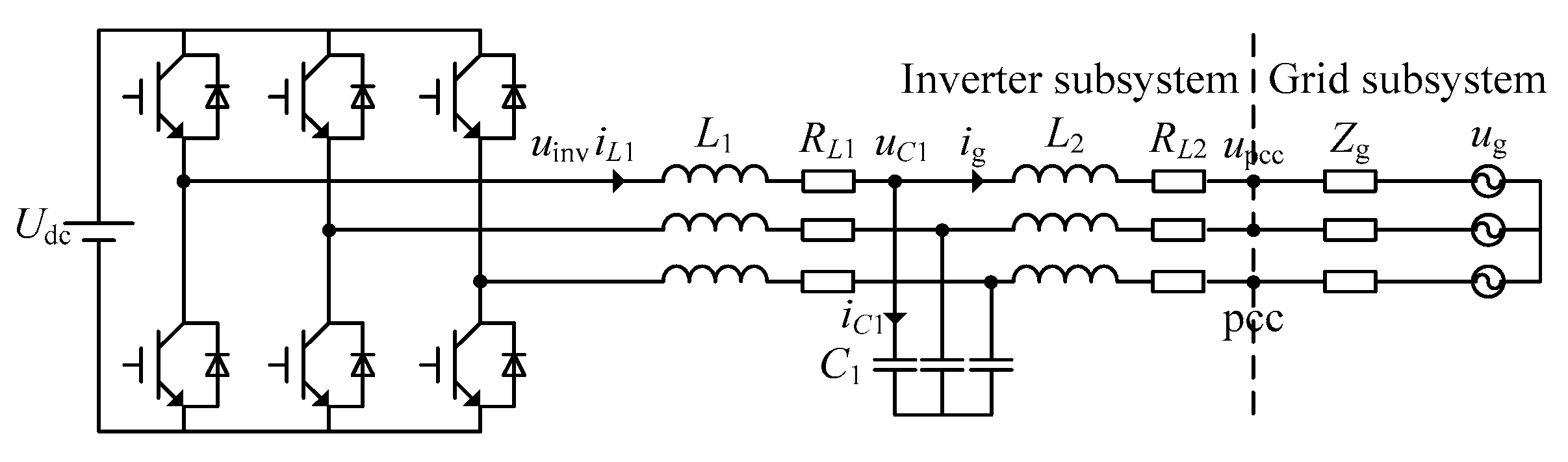
Figure 1 presents the system structure, which includes the inverter subsystem and the grid subsystem. Udc is the DC-side voltage. uinv, uC1 and upcc are the inverter output voltage, filter capacitor voltage and point of common coupling (PCC) voltage. ug is the grid voltage. Zg is the grid impedance. The inductance-capacitance-inductance (LCL) filter is constituted by the inverter-side inductor L1, grid-side inductor L2 and filter capacitor C1. RL1 and RL2 are parasitic resistances of L1 and L2. iL1 is the inverter-side inductor current. ig is the grid-connected current. iC1 is the filter capacitor current.
2.2. Admittance Model of Traditional Control Method
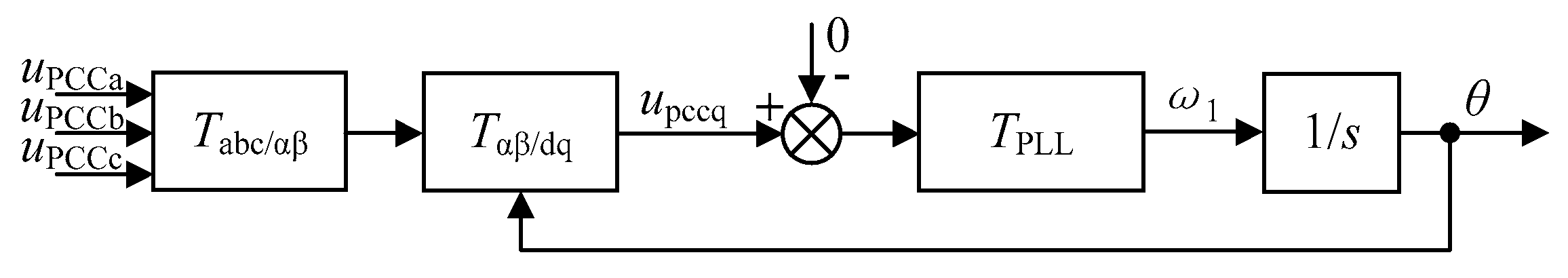
The diagram of the PLL description is shown in Figure 2, where TPLL is the proportional integral (PI) controller of PLL, TPLL = kppll + kipll/s, kppll is the proportional coefficient of PLL PI controller, and kipll is the integral gain of PLL PI controller. Because of the PLL dynamics, there are two dq frames in the system. The first is the system dq frame that is identified by the PCC voltage. The second is the control dq frame that is identified by PLL.
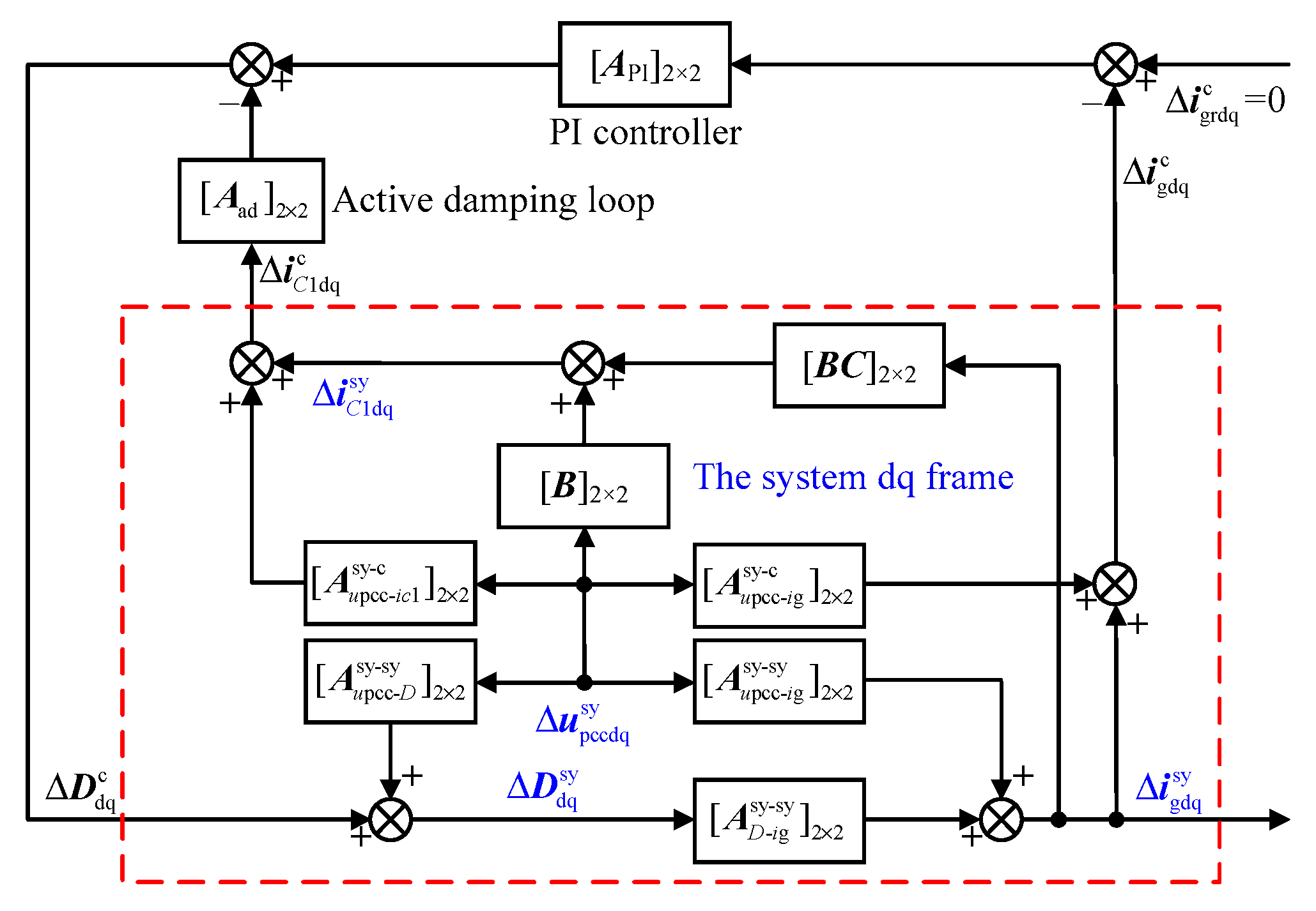
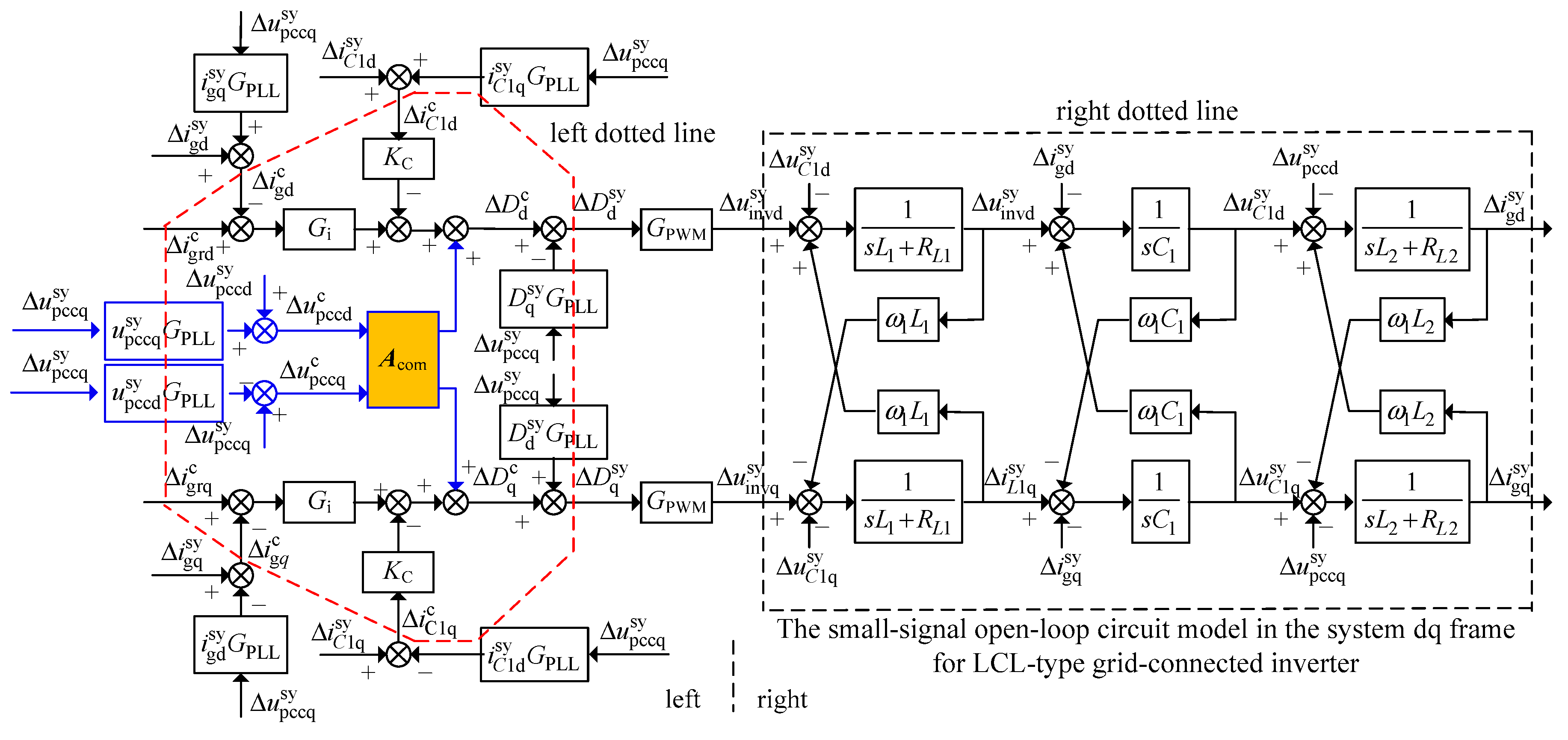
The dq admittance model of the traditional control method, considering the PLL effect, is shown in Figure 3. Outside the dotted line of Figure 3, the control diagram of the traditional control method without considering the PLL effect is pretended. The PI controller [18] is often utilized for the grid-connected current loop due to its simplicity and efficiency. The filter capacitor current feedback [19] is often introduced for the active damping loop to suppress the resonance peak of the LCL filter, which does not require additional passive components or energy loss. However, by adding the small-signal disturbance, PLL affects the grid-connected current vector and filter capacitance current vector in the control dq frame and duty cycle vector in the system dq frame. Therefore, the above vectors are converted between the system dq frame and the control dq frame, and considering the PLL effect, are shown inside the dotted line of Figure 3.
In Figure 3, the superscript variable is “sy,” which represents the variable in the system dq frame, the superscript variable is “c,” which represents the variable in the control dq frame, and the front variable is “∆,” which represents the small-signal variable. The matrices = ∆/∆, = ∆/∆, = ∆/∆, = ∆/∆, = ∆/∆, API is the PI controller matrix of grid-connected current loop and Aad is the active damping coefficient matrix. The derivation of the above matrices are as follows.
The vectors are converted from the system dq frame to the control dq frame via the translation matrix TΔθ, which can be defined as
The small-signal pcc voltage can be obtained as
And (2) can be rewritten as
Combining (3) and (4), the following equation can be obtained as
where .
Substitute (5) into (3), (3) can be obtained as
Similarly, the small-signal duty ratio can be expressed as
And the matrix can be obtained as
Meanwhile, the small-signal grid-connected current can be expressed as
And the matrix can be obtained as
At the same time, the small-signal filter capacitance current can be expressed as
And the matrix can be obtained as
According to the small-signal open-loop circuit model of LCL filter in the system dq frame, the following equation can be expressed as
where
, , .
From (13), (14) can be obtained as
By setting ∆Udc and ∆ to zero, the matrix can be obtained as
where E = [Udc/2, 0; 0, Udc/2].
Similarly, by setting ∆Udc and ∆ to zero, the matrix can be obtained as
where I is the identity matrix.
Meanwhile, the matrix API can be defined as
And the matrix Aad can also be defined as
From Figure 3 and Mason’s gain formula, the inverter output admittance Yinv_PLL with considering the PLL effect using traditional control method can be calculated as
Without considering the PLL effect, = = = 0. The inverter output admittance Yinv using traditional control method can be calculated as
Meanwhile, the PLL equivalent admittance YPLL can be calculated as
2.3. Impedance-Based Stability Criterion
Under the weak grid condition, the grid impedance can be expressed as
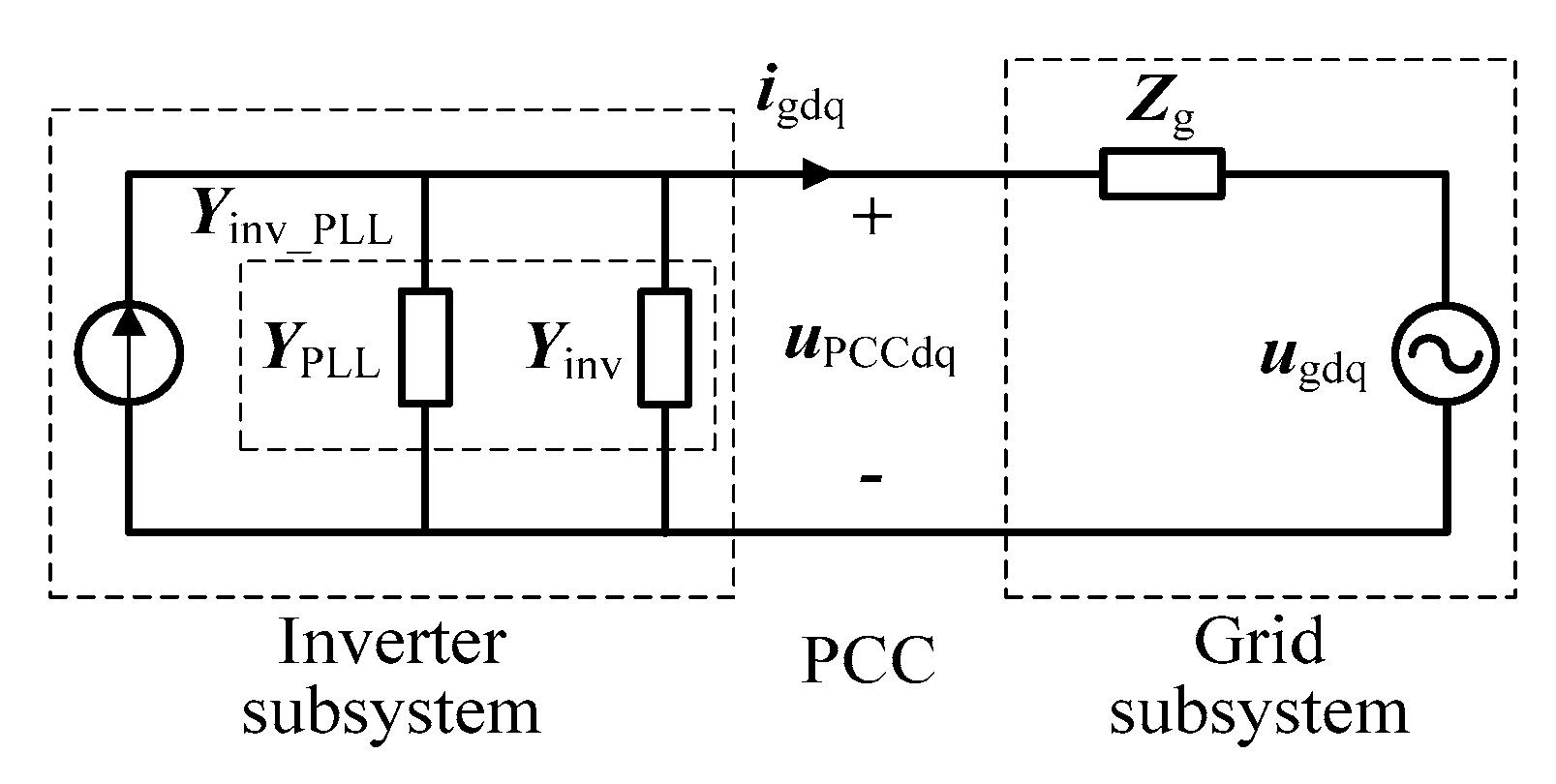
According to the Norton theorem, the equivalent circuit of the system using the traditional control method is shown in Figure 4. The inverter subsystem is equivalent to a parallel connection between the current source and inverter output admittance Yinv_PLL = (Yinv//YPLL). The grid subsystem is equivalent to the grid impedance Zg and an ideal grid in the series connection.
On the basis of the generalized Nyquist criterion [20], if the Nyquist curve for the eigenfunction of the return-ratio matrix L does not encircle (–1, j * 0), the system is in a stable state. L can be depicted as
Therefore, the eigenfunction of the return-ratio matrix L can be calculated as
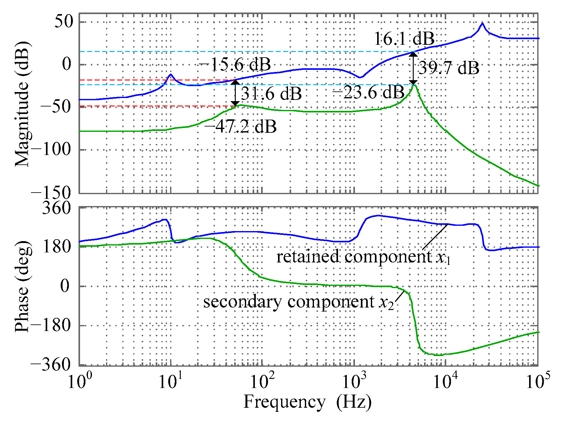
From (24), the retained component x1 and secondary component x2 can be defined as
According to (25), the Bode diagrams of the retained component x1 and secondary component x2 are shown in Figure 5. When the distance between the two is the smallest, the magnitude of x1 is −15.6 dB, the magnitude of x2 is −47.2 dB. The magnitude of x1 is 31.6 dB larger than that of x2, which is equivalent to 38.02 times. Therefore, ignoring the secondary components x2, (24) can be rewritten as
However, a dynamic interconnected system will be formed in the weak grid. The phase margin of the system may be insufficient. That results in increasing the distortion of grid-connected current. To guarantee enough stability and good dynamics, the range of phase margin of the system is usually required to be 30–60° under the weak grid condition.
In the Nyquist curve, the intersection point for the eigenfunction and unit circle is defined as the system cut-off frequency fi, and the location is determined as the phase margin of the system αPM [21]. From (26), αPM can be expressed as
From (27), the system phase margin is increased by decreasing arg(Zgdd(fi)/2) and arg(Ydd(fi) + Yqq(fi)). It is difficult to control the phase of grid impedance arg(Zgdd(fi)/2). Therefore, the target needs to be achieved by decreasing arg(Ydd(fi) + Yqq(fi)).
2.4. Stability Analysis of Traditional Control Method
The Nyquist diagram of the eigenfunction with the traditional control method is shown as in Figure 6. The system cut-off frequency fi is 181 Hz and the system phase margin αPM is 16°, which does not satisfy the requirement of sufficient stability of the system. Therefore, the system phase margin should be improved under the traditional control method.
The Bode diagrams of inverter output admittance Yinv_PLL using the traditional control method are shown in Figure 7. The amplitudes and phases of Ydd, Ydq, Yqd and Yqq can be obtained at the system cut-off frequency, so arg(Ydd(fi) + Yqq(fi)) = 74°. Because the grid impedance is equivalent to the inductance, arg(Zgdd(fi)/2) is generally equal to 90°. According to (27), the system phase margin αPM is 16°, which does not meet sufficient stability of the system. The results are consistent with those in Figure 6. Therefore, the system phase margin should be improved under the traditional control method. Specifically, the PLL shapes the Zqq (1/Yqq) as a negative incremental resistance that may destabilize the system. Meanwhile, |Ydd| and |Yqq| are far larger than |Ydq| and |Yqd|, so |Ydq| and |Yqd| are equal to 0, which verifies the correctness of (23). Within the range of the error, the measurement results are in agreement with the model results, which proves the correctness of the model.
3. Admittance Reshaping Control Methods for Three-Phase Grid-Connected Inverter
3.1. Admittance Reshaping Technique 1 (the Feedforward PCC Voltage)
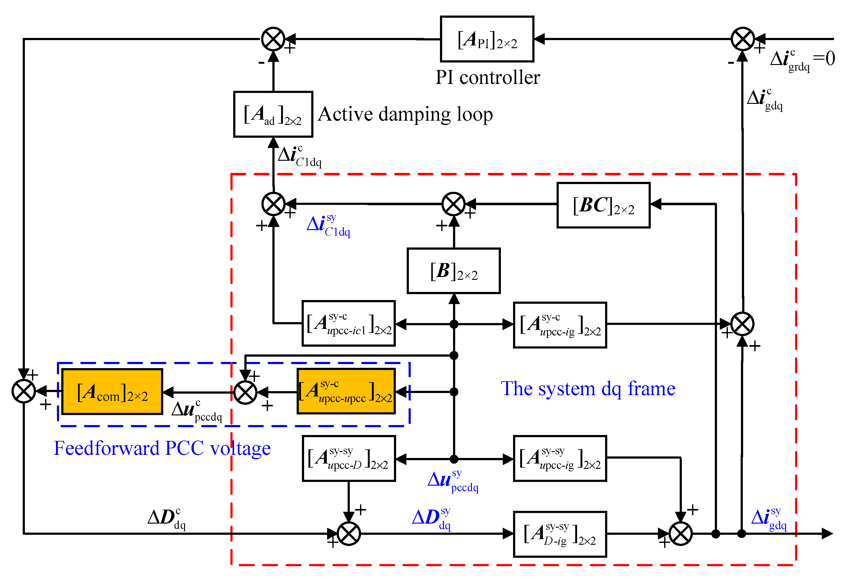
To improve the system’s stability, the proposed admittance reshaping technique 1 uses the feedforward PCC voltage to modify the inverter output admittance Yinv, which is equivalent to adding the virtual admittance to connect in parallel with inverter output admittance. The system diagram of the proposed admittance reshaping technique 1—considering the effect of PLL—is shown in Figure 8. Inside the left dotted line of Figure 8, the control diagram of the proposed admittance reshaping technique 1—without considering the PLL effect—is presented. The vectors are converted between the system dq frame and the control dq frame that considers the PLL effect are shown outside the left dotted line of Figure 8.
From Figure 8, the dq admittance model of the proposed admittance reshaping technique 1 is obtained, as shown in Figure 9, where the matrix can be obtained as
Therefore, the inverter output admittance Yinvc_PLL with the proposed admittance reshaping technique 1 can be expressed as
Without considering the PLL effect, = = = 0. The inverter output admittance Yinvc using the proposed admittance reshaping technique 1 can be calculated as
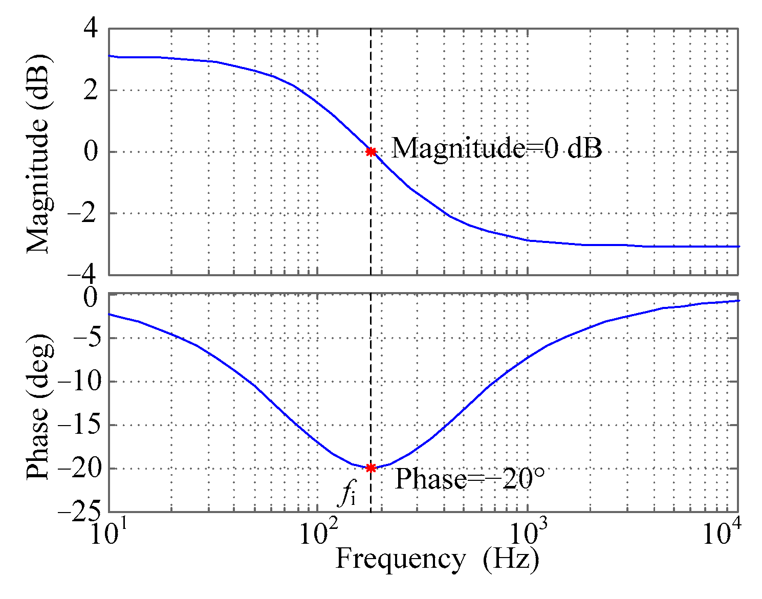
Next, the calculation process of the feedforward matrix Acom is introduced. The optimization function Gp(s) of the inverter output admittance phase, which can be given as
where kp is the proportional coefficient, kω is the phase coefficient, and km is the gain coefficient. kp and kω can reduce the phase at the desired frequency and km can compensate for the amplitude offset at the desired frequency.
The Bode diagram of the optimization function Gp(s) is shown in Figure 10. By selecting the appropriate parameters, the amplitude of Gp(s) is 0 dB at the desired frequency and the phase reaches the minimum at the desired frequency.
Meanwhile, the optimization matrix Ap can be defined as
If the series correction between the optimization matrix Ap and inverter output admittance Yinv_PLL is taken, the aim of compensating for the phase of inverter output admittance at the desired frequency will be realized. Meanwhile, the feedforward matrix Acom can also be obtained. Therefore, the inverter output admittance Yinvc_PLL with using the proposed admittance reshaping technique 1 can be rewritten as
Therefore, Gcomdd in the feedforward matrix can be expressed as
where and .
Meanwhile, Gcomqq in the feedforward matrix can also be expressed as
where .
Using the proposed admittance reshaping technique 1, Yinvc_PLL is equivalent to the parallel connection between YPLL and Yinvc. Therefore, the proposed admittance reshaping technique 1 is equivalent to adding the virtual admittance to connect in parallel with inverter output admittance Yinv.
The Bode diagrams of inverter output admittances Yinvc_PLL with the proposed admittance reshaping technique 1 are shown in Figure 11, where arg(Ycdd(fi) + Ycqq(fi)) = 54°. Because the grid impedance is equivalent to the inductance, arg(Zgdd(fi)/2) is generally equal to 90°. According to (27), the system phase margin αPM is 36°, which meets sufficient stability of the system. Therefore, the proposed admittance reshaping technique 1 increases the system phase margin. At the same time, the measurement results are in good agreement with the modified model, which proves the correctness of the modified model.
3.2. Admittance Reshaping Technique 2 (the Active Damping Controller)
To increase the system phase margin, the proposed admittance reshaping technique 2 adopts the active damping controller to reconstruct the PLL equivalent admittance YPLL. The control block diagram of the improved PLL is shown in Figure 12. The proposed admittance reshaping technique 2 reduces the phase of PLL equivalent admittance at the system cut-off frequency, which improves system stability.
From Figure 12, the closed-loop transfer function of PLL GPLLc using the proposed admittance reshaping technique 2 can be expressed as
Therefore, the matrix in (8) can be rewritten as
Meanwhile, the matrix in (10) can be rewritten as
At the same time, the matrix in (12) can be rewritten as
Therefore, the inverter output admittance Yinv_PLLc using the proposed admittance reshaping technique 2 can be expressed as
Next, the calculation process of the active damping controller GAD is introduced. According to (32), the closed-loop transfer function of PLL GPLLc using the proposed admittance reshaping technique 2 can be rewritten as
Therefore, the active damping controller GAD can be obtained as
Using proposed admittance reshaping technique 2, Yinv_PLLc is equivalent to the parallel connection between YPLLc and Yinv. Therefore, the proposed admittance reshaping technique 2 is equivalent to adding the virtual admittance to connect in parallel with the PLL equivalent admittance YPLL. Using the proposed admittance reshaping technique 2, the reconstructed inverter output admittances Yinv_PLLc can achieve the same purpose as proposed admittance reshaping technique 1.
3.3. Design Method of Control Parameters
By selecting the appropriate parameters kp and kω, the phase of the inverter output admittance is reduced at the system cut-off frequency, which increases the system phase margin. In addition, the amplitude of the inverter output admittance at the system cut-off frequency will be changed. Therefore, it is essential to select the appropriate parameter km to compensate for the amplitude offset.
The phase-frequency function of Gp(s) is expressed as
If dϕp(ω)/dω = 0, the maximum compensation angular frequency ωm can be obtained as
Combining (44) and (45), the maximum compensation phase ϕm can be derived as
To maintain the amplitude of the inverter output admittance at the system cut-off frequency, the amplitude of Gp(s) should be 0 dB at the system cut-off frequency, that is, |Gp(j2πfi)| = 1. The gain coefficient of phase compensation km can be expressed as
Using the traditional control method, the system cut-off frequency fi is 181 Hz, and the system phase margin αPM is 16°, which does not meet sufficient stability of the system. The parameter design process of the proposed control methods can be illustrated as follows. Firstly, the maximum compensation phase frequency ωm should be equivalent to the system cut-off angular frequency ωi = 2πfi ≈ 1137rad/s. Secondly, the range of maximum compensation phase ϕm is −14~−44° on the basis of the required system phase margin. Then, the range of kp is 1.6383~5.55 by (46). Next, the range of kω is 3.7325 × 10⁻⁴−6.8698 × 10−4 by (45). Finally, the range of km is 1.28–2.3558 by (47).
3.4. Contrast Analysis of System Stability
The Nyquist diagrams of the eigenfunction are shown in Figure 13. Using the traditional control method, the system phase margin αPM is separately 16°. Using the proposed control methods, the system phase margins αPM are separately 30° and 60°, which are increased by 14° and 44°, respectively. The result is the same as the designed maximum compensation phase, which meets sufficient stability and good dynamics of the system.
4. Experiments Verification
To prove the validity of the theoretical analysis, the experimental platform for a three-phase grid-connected system was built, as shown in Figure 14a, which included a three-phase grid-connected inverter, a detection and data acquisition circuit (voltage and current sensors), and an industrial personal computer. The three-phase grid-connected inverter in Figure 14b includes the main circuit, control board and LCL filter circuit. The system parameters are shown in Table 1.
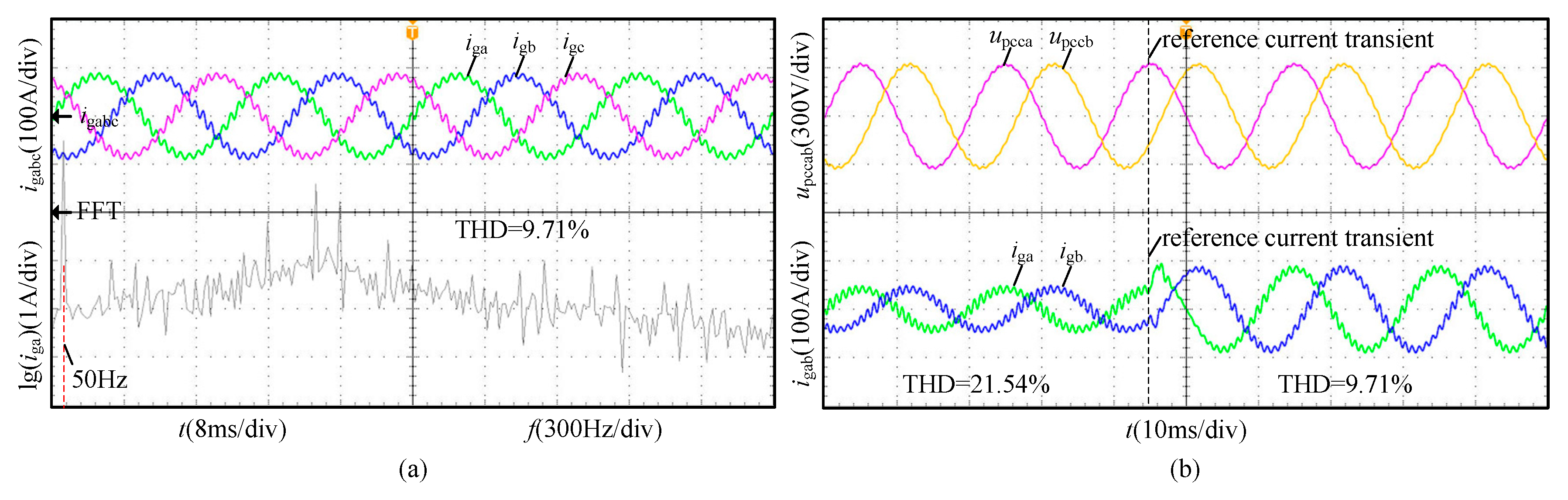
To improve the stable operation range, the stability enhancement method was proposed [14] by largely reducing the PLL bandwidth, abbreviated as the traditional control method. The traditional control method, the proposed admittance reshaping techniques 1 and 2, the experimental waveforms of PCC voltage upcc and the grid-connected current ig are shown in Figure 15, Figure 16 and Figure 17. The experimental results of the grid-connected current in the three cases are shown in Table 2.
In the case of the traditional control method from Figure 15a, the total harmonic distortion (THD) of the steady-state grid-connected current is 9.71%. The harmonic contents of the grid-connected current are large. The reason is that the phase margin of the system may be insufficient using the traditional control method. Therefore, it is essential to propose the control method to increase the system phase margin.
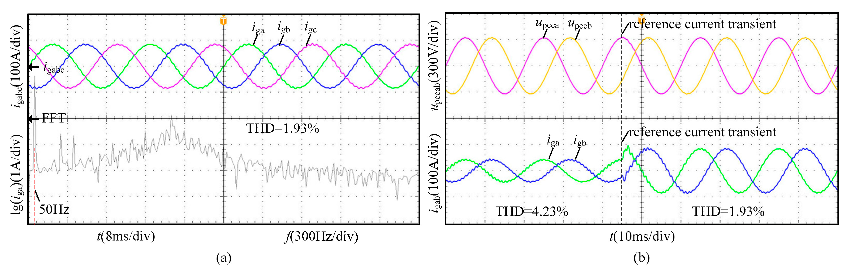
To increase the system phase margin, admittance reshaping techniques 1 and 2 are proposed, which use a set of parameters within the design range shown in Table 3. In the case of the proposed admittance reshaping techniques 1 and 2 from Figure 16a and Figure 17a, the THD of the steady-state grid-connected currents are 1.72% and 1.93%. In both cases, the harmonic contents of the grid-connected current are greatly attenuated. The reason is that the proposed admittance reshaping techniques 1 and 2 increase the system damping and improve system stability. Therefore, the validity of the theoretical analysis is verified.
As can be seen in Figure 15b, Figure 16b and Figure 17b, the reference grid-connected current increases from 36.5A to 73A in the case of the traditional control method and the proposed admittance reshaping techniques 1 and 2. The transient experimental results in the three cases are similar. Therefore, compared with the traditional control method, the proposed admittance reshaping techniques 1 and 2 can ensure system dynamics.
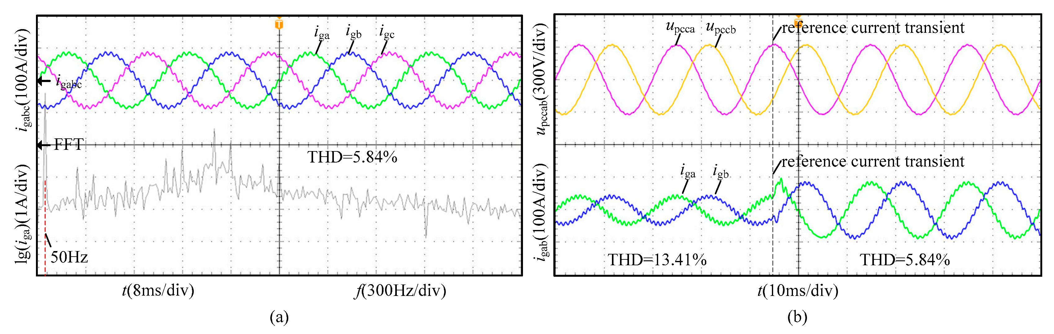
To verify the reasonableness of the parameter design for the proposed admittance reshaping techniques 1 and 2, another set of parameters without the design range is shown in Table 3. The experimental waveforms of PCC voltage upcc and grid-connected current ig in both cases are shown as Figure 18 and Figure 19. The experimental results of the grid-connected current in both cases are shown in Table 2.
From Figure 18a and Figure 19a, the THD of the steady-state grid-connected current is 5.62% and 5.84% in the case of the proposed control methods without the design range. The THD of the grid-connected current in both cases is less than that in Figure 15a with the traditional control method, but greater than that in Figure 16a and Figure 17a within the design range. The reason is that the phase margin of the system has been improved but it has not yet met sufficient stability of the system. Therefore, the reasonableness of the parameter design is verified for the proposed control methods.
As can be seen in Figure 15b, Figure 18b and Figure 19b, the reference grid-connected current increases from 36.5 A to 73 A and the transient experimental results in the three cases are similar. Therefore, compared with the traditional control method, the proposed control methods without the design range can also ensure the system dynamics.
5. Conclusions
The negative impact of PLL on system stability is caused by the range of negative incremental resistance. It will increase impedance coupling between inverters and grid, which reduces the system phase margin or leads to system instability. Therefore, two admittance reshaping control methods that consider the PLL effect are proposed to improve system damping. The first reshaping technique uses the feedforward PCC voltage to modify the inverter output admittance. The second reshaping technique adopts the active damping controller to reconstruct the PLL equivalent admittance. The proposed control methods not only increase the system phase margin but also ensure the system dynamic response speed. The total harmonic distortion of the steady-state grid-connected current is reduced to less than 2%. Furthermore, a specific design method of control parameters is depicted. Finally, experimental results are provided to prove the validity of the proposed control methods. Still, the paper does not study the effect of time delay on the proposed control methods, which is an important topic to be explored in the future.
Author Contributions
L.Y. and Y.C. provided the original idea for this paper. L.Y., A.L. and K.H. organized the manuscript and attended the discussions when analysis and verification were carried out. All the authors gave comments and suggestions for the writing of and descriptions in the manuscript.
Funding
This research was supported by the National Key R&D Program of China under Grant No. 2017YFB0902000, and the Science and Technology Project of State Grid under Grant No. SGXJ0000KXJS1700841.
Conflicts of Interest
The authors declare no conflict of interest.
References
- Guo, X.; Yang, Y.; Zhang, X. Advanced control of grid-connected current source converter under unbalanced grid voltage conditions. IEEE Trans. Ind. Electron. 2018, 65, 9225–9233. [Google Scholar] [CrossRef]
- Zhang, D.; Li, J.; Hui, D. Coordinated control for voltage regulation of distribution network voltage regulation by distributed energy storage systems. Prot. Control Mod. Power Syst. 2018, 3, 35–42. [Google Scholar] [CrossRef]
- Guo, X.; Yang, Y.; Zhu, T. ESI: A novel three-phase inverter with leakage current attenuation for transformerless PV systems. IEEE Trans. Ind. Electron. 2018, 65, 2967–2974. [Google Scholar] [CrossRef]
- Fan, L.; Miao, Z. An explanation of oscillations due to wind power plants weak grid interconnection. IEEE Trans. Sustain. Energy 2018, 9, 488–490. [Google Scholar] [CrossRef]
- Yang, L.; Chen, Y.; Wang, H.; Luo, A.; Huai, K. Oscillation suppression method by two notch filters for parallel inverters under weak grid conditions. Energies 2018, 11, 3441. [Google Scholar] [CrossRef]
- Han, Y.; Chen, H.; Li, Z.; Yang, P.; Xu, L.; Guerrero, J.M. Stability analysis for the grid-connected single-phase asymmetrical cascaded multilevel inverter with SRF-PI current control under weak grid conditions. IEEE Trans. Power Electron. 2019, 34, 2052–2069. [Google Scholar] [CrossRef]
- Zhou, X.; Zhou, L.; Chen, Y.; Shuai, Z.; Guerrero, J.M.; Luo, A.; Wu, W.; Yang, L. Robust grid-current-feedback resonance suppression method for LCL-type grid-connected inverter connected to weak grid. IEEE J. Emerg. Sel. Top. Power Electron. 2018, 6, 2126–2137. [Google Scholar] [CrossRef]
- Cao, W.; Ma, Y.; Wang, F. Sequence-impedance-based harmonic stability analysis and controller parameter design of three-phase inverter-based multibus AC power systems. IEEE Trans. Power Electron. 2017, 32, 7674–7693. [Google Scholar] [CrossRef]
- Wu, W.; Zhou, L.; Chen, Y.; Luo, A.; Dong, Y.; Zhou, X.; Xu, Q.; Yang, L.; Guerrero, J.M. Sequence-impedance-based stability comparison between VSGs and traditional grid-connected inverters. IEEE Trans. Power Electron. 2019, 34, 46–52. [Google Scholar] [CrossRef]
- Liu, H.; Xie, X.; Liu, W. An oscillatory stability criterion based on the unifieddq-frame impedance network model for power systems with high-penetration renewables. IEEE Trans. Power Syst. 2018, 33, 3472–3485. [Google Scholar] [CrossRef]
- Shuai, Z.; Li, Y.; Wu, W.; Tu, C.; Luo, A.; Shen, Z.J. Divided DQ small-signal model: A new perspective for the stability analysis of three-phase grid-tied inverters. IEEE Trans. Ind. Electron. 2019, 66, 6493–6504. [Google Scholar] [CrossRef]
- He, J.; Li, Y.W. Analysis, design, and implementation of virtual impedance for power electronics interfaced distributed generation. IEEE Trans. Ind. Appl. 2011, 47, 2525–2538. [Google Scholar] [CrossRef]
- Dannehl, J.; Liserre, M.; Fuchs, F.W. Filter-based active damping of voltage source converters with LCL filter. IEEE Trans. Ind. Electron. 2011, 58, 3623–3633. [Google Scholar] [CrossRef]
- Zhou, J.Z.; Ding, H.; Fan, S.; Zhang, Y.; Gole, A.M. Impact of short-circuit ratio and phase-locked-loop parameters on the small-signal behavior of a VSC-HVDC converter. IEEE Trans. Power Deliv. 2014, 29, 2287–2296. [Google Scholar] [CrossRef]
- Golestan, S.; Guerrero, J.M.; Abusorrah, A.M.; Al-Turki, Y. Hybrid synchronous/stationary reference-frame-filtering-based PLL. IEEE Trans. Ind. Electron. 2015, 62, 5018–5022. [Google Scholar] [CrossRef]
- Wang, F.; Duarte, J.L.; Hendrix, M.A.M.; Ribeiro, P.F. Modeling and analysis of grid harmonic distortion impact of aggregated DG inverters. IEEE Trans. Power Electron. 2011, 26, 786–797. [Google Scholar] [CrossRef]
- Chen, M.; Peng, L.; Wang, B.; Kan, J. PLL based on extended trigonometric function delayed signal cancellation under various adverse grid conditions. IET Power Electron. 2018, 11, 1689–1697. [Google Scholar] [CrossRef]
- Selvaraj, J.; Rahim, N.A. Multilevel inverter for grid-connected PV system employing digital PI controller. IEEE Trans. Ind. Electron. 2009, 56, 149–158. [Google Scholar] [CrossRef]
- Zhang, N.; Tang, H.; Yao, C. A systematic method for designing a PR controller and active damping of the LCL filter for single-phase grid-connected PV inverters. Energies 2014, 7, 3934–3954. [Google Scholar] [CrossRef]
- Belkhayat, M. Stability Criteria for AC Power Systems with Regulated Loads. Ph.D. Thesis, Purdue University, West Lafayette, IN, USA, 1997. [Google Scholar]
- Kuo, B.C.; Golnaraghi, F. Automatic Control Systems; Prentice-Hall: Englewood Cliffs, NJ, USA, 1995; pp. 365–373. [Google Scholar]
Figure 1.
Three-phase grid-connected system.

Figure 2.
The diagram of PLL description.

Figure 3.
The dq admittance model of traditional control method.

Figure 4.
Equivalent circuit of the system with the traditional control method.

Figure 5.
The Bode diagrams of the retained component x1 and secondary component x2.

Figure 6.
The Nyquist diagram of the eigenfunction with the traditional control method.
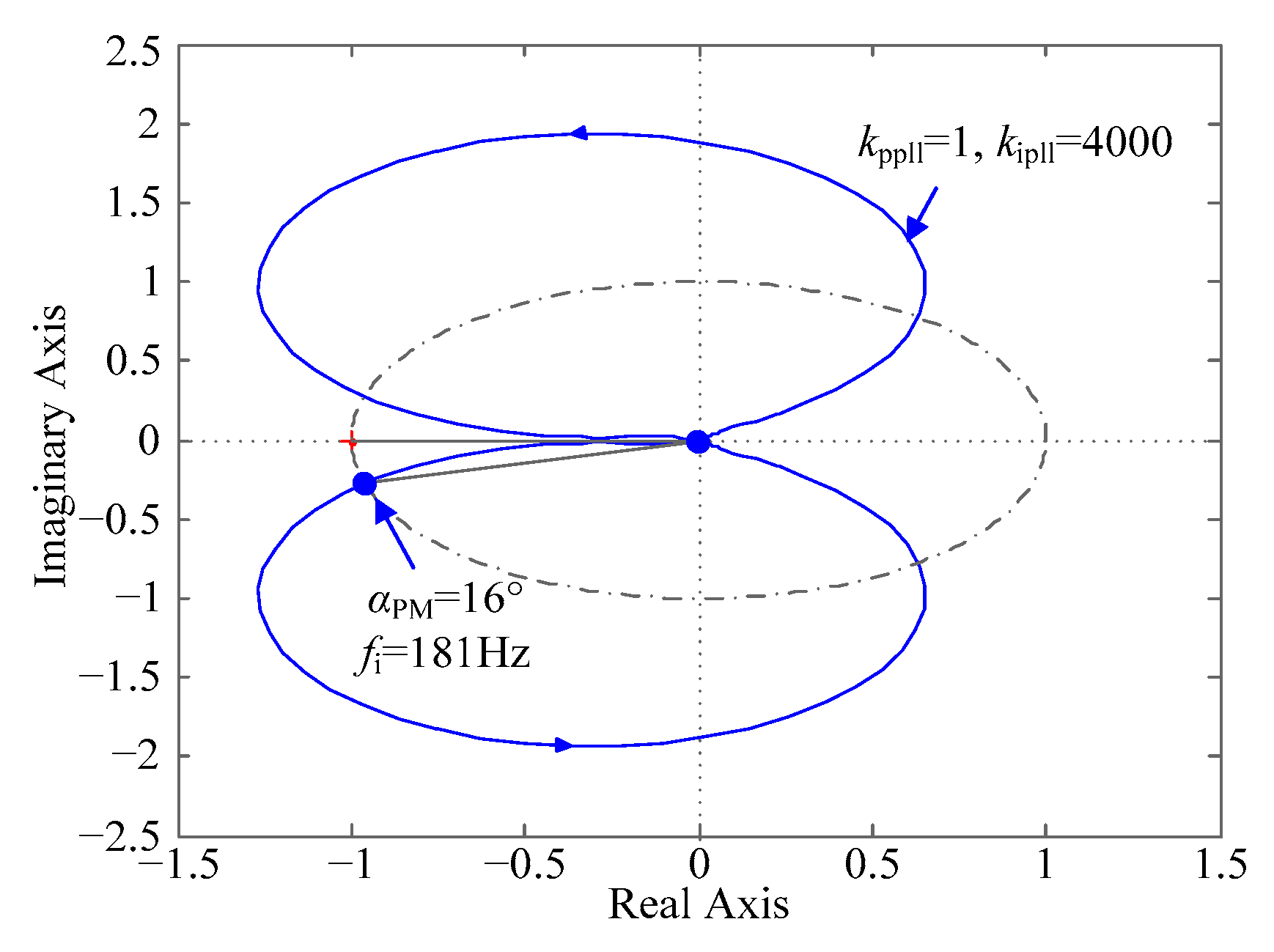
Figure 7.
The Bode diagrams of inverter output admittance Yinv_PLL of traditional control method. (a) Ydd; (b) Yqd; (c) Ydq; (d) Yqq.
Figure 7.
The Bode diagrams of inverter output admittance Yinv_PLL of traditional control method. (a) Ydd; (b) Yqd; (c) Ydq; (d) Yqq.
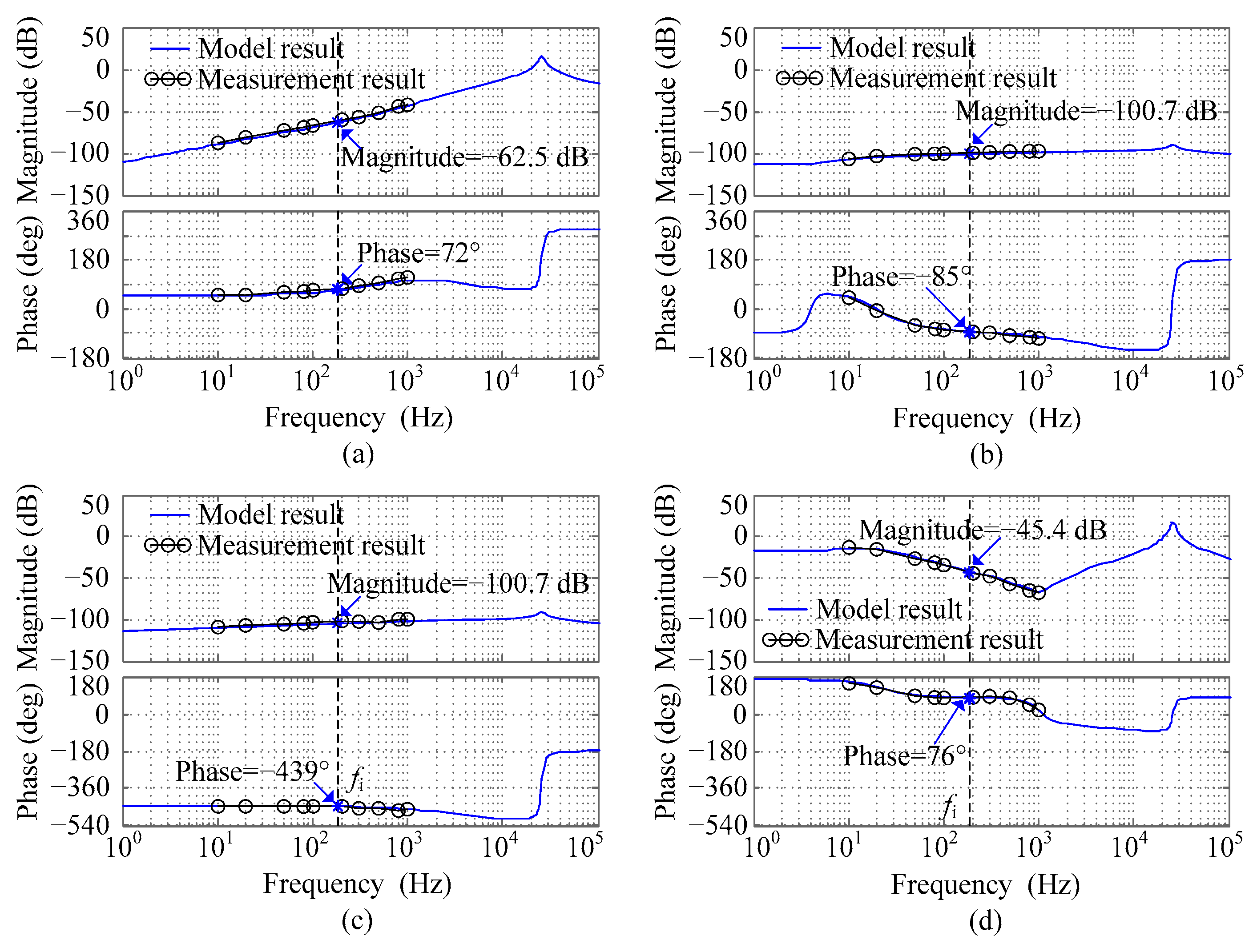
Figure 8.
The system diagram of proposed admittance reshaping technique 1 considering the phase-locked loop (PLL) effect.
Figure 8.
The system diagram of proposed admittance reshaping technique 1 considering the phase-locked loop (PLL) effect.

Figure 9.
The dq admittance model of proposed admittance reshaping technique 1.

Figure 10.
The Bode diagram of the optimization function Gp(s).

Figure 11.
The Bode diagrams of inverter output admittances Yinvc_PLL with proposed admittance reshaping technique 1. (a) Ycdd; (b) Ycqd; (c) Ycdq; (d) Ycqq.
Figure 11.
The Bode diagrams of inverter output admittances Yinvc_PLL with proposed admittance reshaping technique 1. (a) Ycdd; (b) Ycqd; (c) Ycdq; (d) Ycqq.
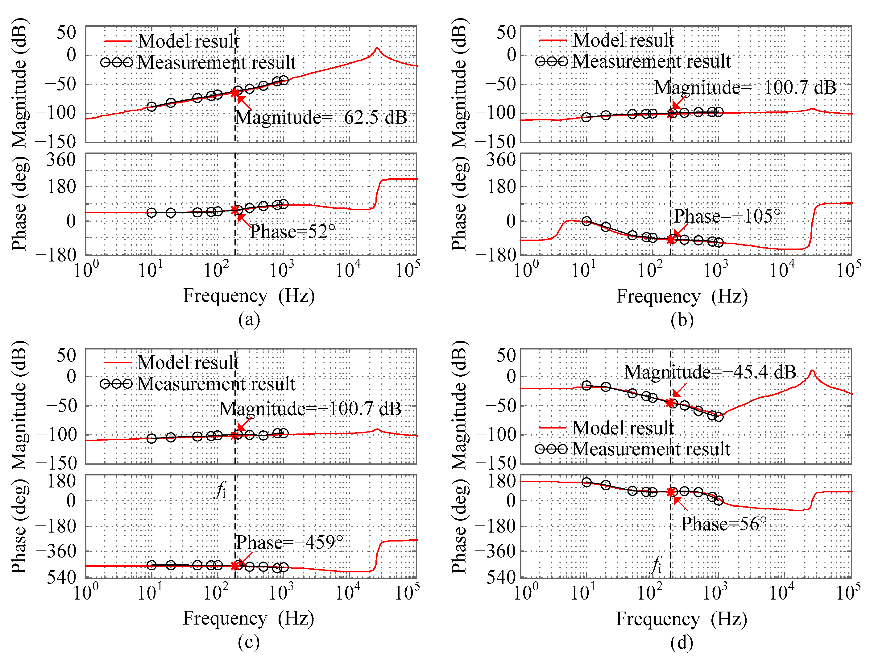
Figure 12.
The control block diagram of the improved PLL.
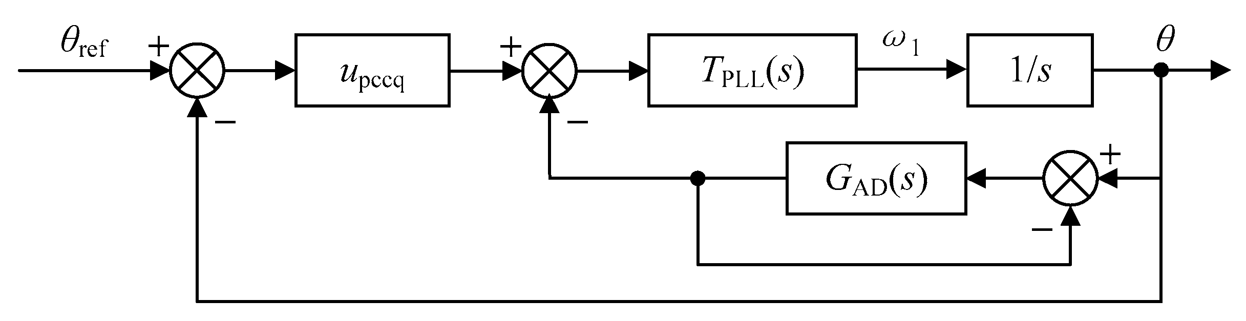
Figure 13.
The Nyquist diagrams of the eigenfunction.
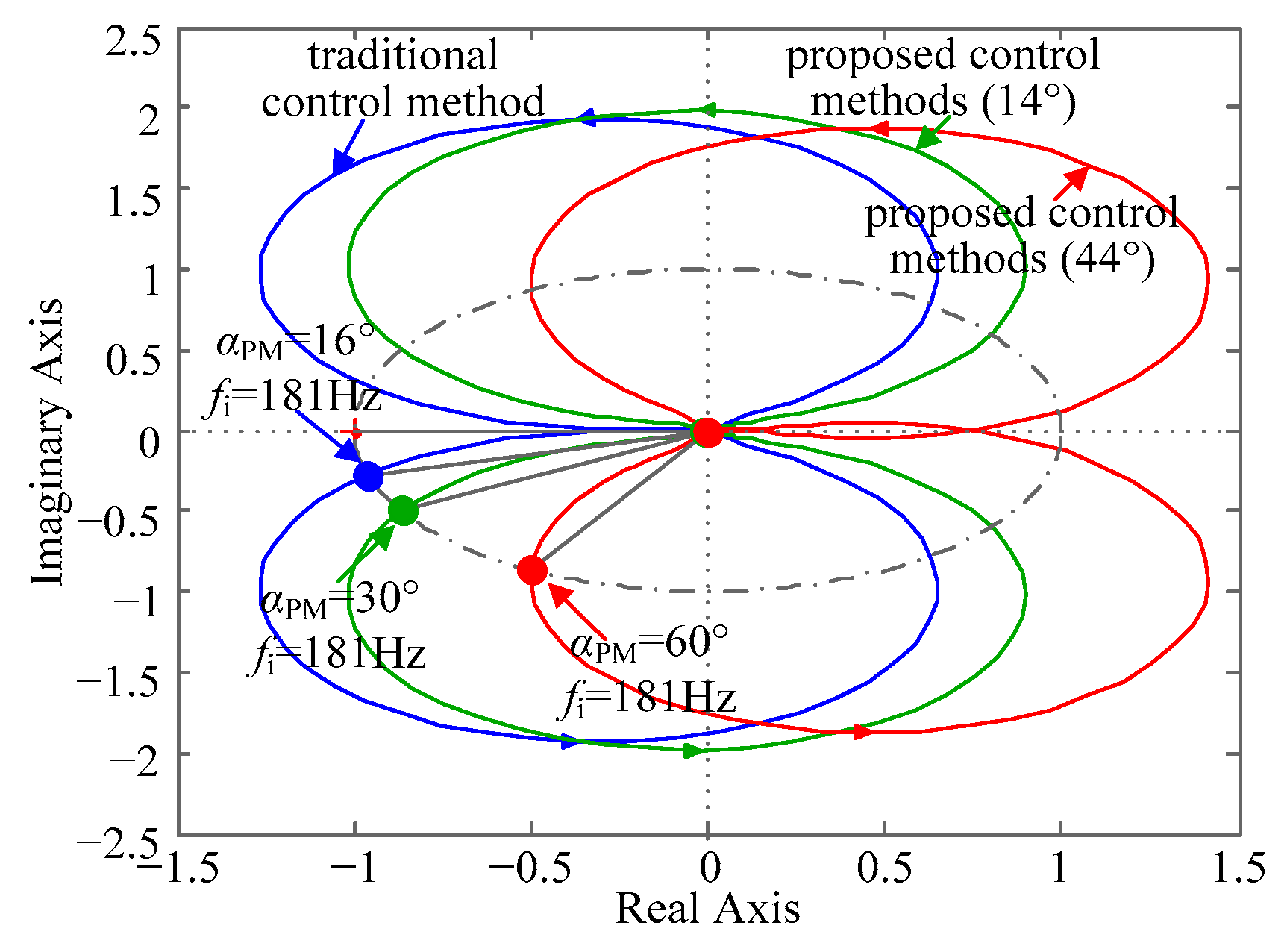
Figure 14.
Experimental platform for a three-phase grid-connected system. (a) Whole; (b) Details.
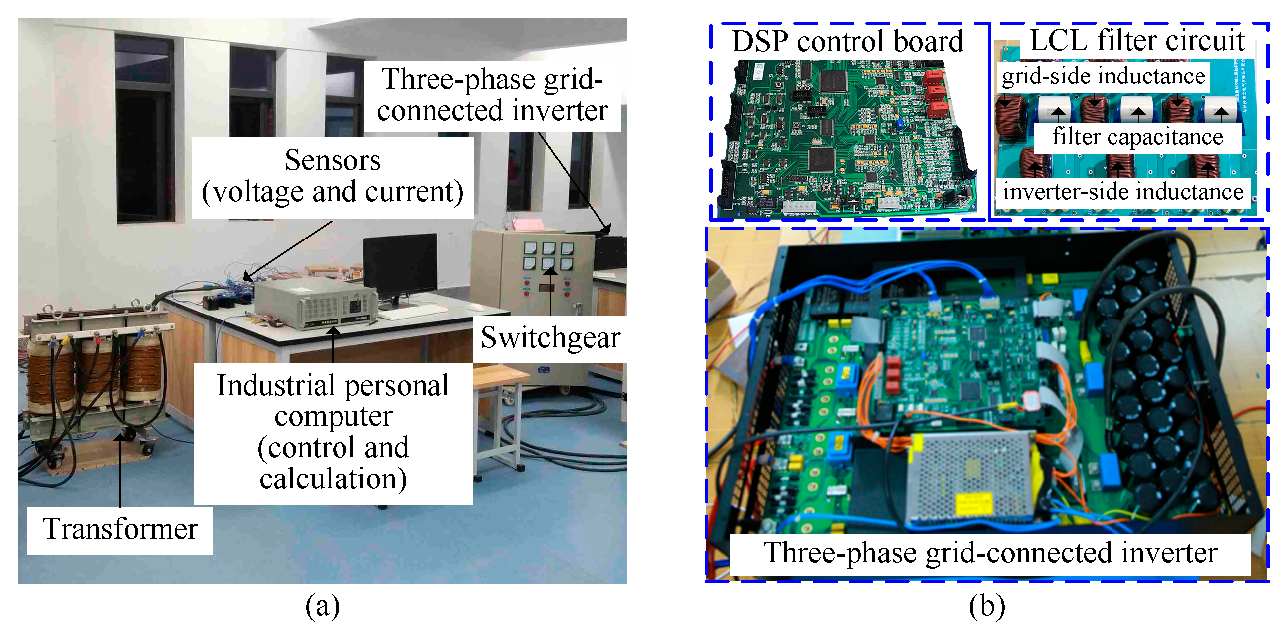
Figure 15.
Experimental waveforms of point of common coupling (PCC) voltage upcc and grid-connected current ig with traditional control method. (a) Steady state; (b) Transient.
Figure 15.
Experimental waveforms of point of common coupling (PCC) voltage upcc and grid-connected current ig with traditional control method. (a) Steady state; (b) Transient.

Figure 16.
Experimental waveforms of upcc and ig with proposed admittance reshaping technique 1 within the parameter design range. (a) Steady state; (b) Transient.
Figure 16.
Experimental waveforms of upcc and ig with proposed admittance reshaping technique 1 within the parameter design range. (a) Steady state; (b) Transient.
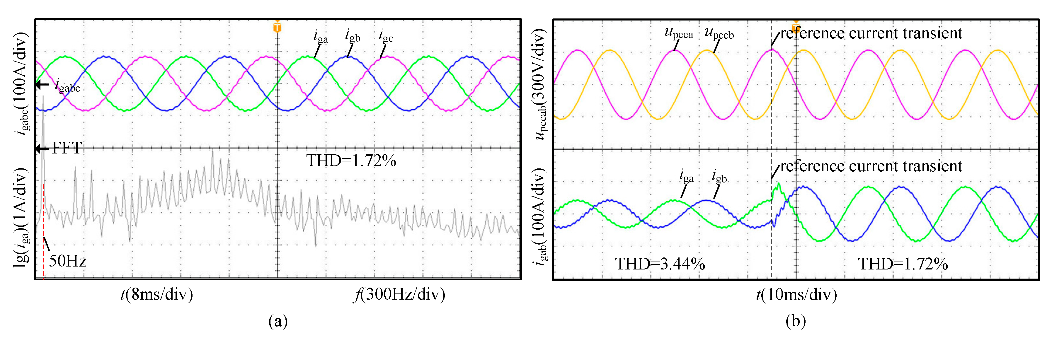
Figure 17.
Experimental waveforms of upcc and ig with proposed admittance reshaping technique 2 within the parameter design range. (a) Steady state; (b) Transient.
Figure 17.
Experimental waveforms of upcc and ig with proposed admittance reshaping technique 2 within the parameter design range. (a) Steady state; (b) Transient.

Figure 18.
Experimental waveforms of upcc and ig with proposed admittance reshaping technique 1 without the parameter design range. (a) Steady state; (b) Transient.
Figure 18.
Experimental waveforms of upcc and ig with proposed admittance reshaping technique 1 without the parameter design range. (a) Steady state; (b) Transient.
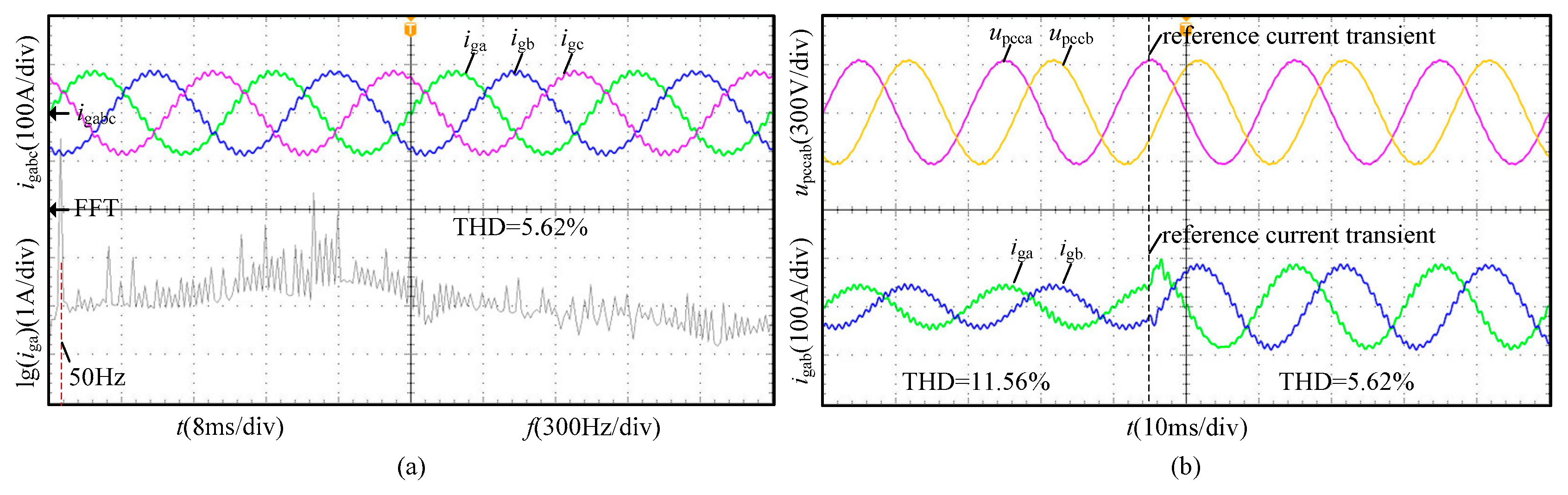
Figure 19.
Experimental waveforms of upcc and ig with proposed admittance reshaping technique 2 without the parameter design range. (a) Steady state; (b) Transient.
Figure 19.
Experimental waveforms of upcc and ig with proposed admittance reshaping technique 2 without the parameter design range. (a) Steady state; (b) Transient.


Table 1.
System parameters.
| Parameter/Unit | Value |
|---|---|
| DC voltage Udc/V | 720 |
| Inverter-side inductor L1/mH, RL1/Ω | 0.6, 0.01 |
| Filter capacitor C1/μF | 10 |
| Grid-side inductor L2/mH, RL2/Ω | 0.15, 0.001 |
| Grid inductor Lg/mH | 0.05 |
| Grid-connected current reference igrd, igrq/A | −73, 0 |
| Grid-connected current , /A | −73, 0 |
| PCC voltage , /V | 311, 0 |
| Filter capacitor current , /A | 0.03, 0.90 |
| Duty radio , | 0.55, 0.01 |
| PLL PI controller kppll, kipll | 1, 4000 |
| Grid current loop PI controller kpi, kii | 0.45, 1000 |
| Active damping coefficient KC | 1.15 |
| Fundamental frequency f1/Hz | 50 |
| Switching frequency fs/kHz | 10 |
Table 2.
The experimental results of the grid-connected current.
| Case | THD of the Steady-State Grid-Connected Current |
|---|---|
| Traditional control method | 9.71% |
| Admittance reshaping technique 1 (within the parameter design range) | 1.72% |
| Admittance reshaping technique 2 (within the parameter design range) | 1.93% |
| Admittance reshaping technique 1 (without the parameter design range) | 5.62% |
| Admittance reshaping technique 2 (without the parameter design range) | 5.84% |
Table 3.
Different sets of parameters.
| Case | ϕm | kp | kω | km |
|---|---|---|---|---|
| within the design range | −20° | 2.04 | 6.16 × 10⁻⁴ | 1.43 |
| without the design range | −10° | 1.42 | 7.38 × 10⁻⁴ | 1.19 |
© 2019 by the authors. Licensee MDPI, Basel, Switzerland. This article is an open access article distributed under the terms and conditions of the Creative Commons Attribution (CC BY) license (http://creativecommons.org/licenses/by/4.0/).
Share and Cite
MDPI and ACS Style
Yang, L.; Chen, Y.; Luo, A.; Huai, K. Admittance Reshaping Control Methods to Mitigate the Interactions between Inverters and Grid. Energies 2019, 12, 2457. https://doi.org/10.3390/en12132457
AMA Style
Yang L, Chen Y, Luo A, Huai K. Admittance Reshaping Control Methods to Mitigate the Interactions between Inverters and Grid. Energies. 2019; 12(13):2457. https://doi.org/10.3390/en12132457
Chicago/Turabian StyleYang, Ling, Yandong Chen, An Luo, and Kunshan Huai. 2019. "Admittance Reshaping Control Methods to Mitigate the Interactions between Inverters and Grid" Energies 12, no. 13: 2457. https://doi.org/10.3390/en12132457
Note that from the first issue of 2016, this journal uses article numbers instead of page numbers. See further details here.