Optimal Residential Load Scheduling Under Utility and Rooftop Photovoltaic Units

Abstract

With the rapid advancement in technology, electrical energy consumption is increasing rapidly. Especially, in the residential sector, more than 80% of electrical energy is being consumed because of consumer negligence. This brings the challenging task of maintaining the balance between the demand and supply of electric power. In this paper, we focus on the problem of load balancing via load scheduling under utility and rooftop photovoltaic (PV) units to reduce electricity cost and peak to average ratio (PAR) in demand-side management. For this purpose, we adopted genetic algorithm (GA), binary particle swarm optimization (BPSO), wind-driven optimization (WDO), and our proposed genetic WDO (GWDO) algorithm, which is a hybrid of GA and WDO, to schedule the household load. For energy cost estimation, combined real-time pricing (RTP) and inclined block rate (IBR) were used. The proposed algorithm shifts load from peak consumption hours to off-peak hours based on combined pricing scheme and generation from rooftop PV units. Simulation results validate our proposed GWDO algorithm in terms of electricity cost and PAR reduction while considering all three scenarios which we have considered in this work: (1) load scheduling without renewable energy sources (RESs) and energy storage system (ESS), (2) load scheduling with RESs, and (3) load scheduling with RESs and ESS. Furthermore, our proposed scheme reduced electricity cost and PAR by 22.5% and 29.1% in scenario 1, 47.7% and 30% in scenario 2, and 49.2% and 35.4% in scenario 3, respectively, as compared to unscheduled electricity consumption.

1. Introduction

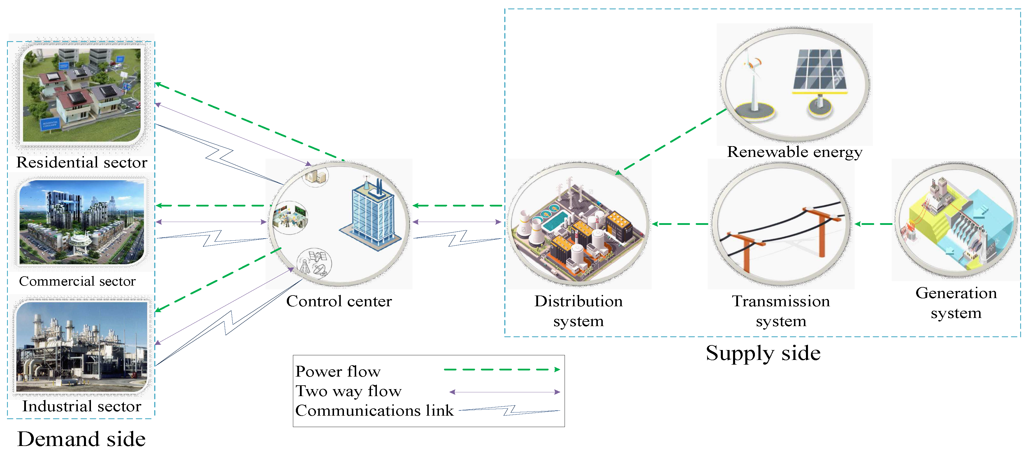
The global energy demand drastically increases on a daily basis, and fossil fuels are limited and being exhausted. The smart grid (SG) emerged as a smart solution that accommodates information communication technology (ICT), fossil fuels generation, renewable energy (RE) generation, and hybrid generation, as shown in Figure 1. Therefore, it is important to increase the utilization of RE sources (RESs) because of environmental issues and the need to reduce carbon emission. Federal energy regulatory commission (FERC) passed renewable portfolio standards to increase production from RESs. Under renewable portfolio standards, the utility companies and energy providers in the U.S. and the U.K. serve some of the consumers’ load with RESs [1]. Among the various types of RESs, solar is the most abundant, free of cost, and available everywhere to everyone. As recently as 2014 the use of RESs had increased; it was recorded that Denmark generated 60%, Spain generated 29%, and Portugal generated 30% of electricity from RESs. A system with a high penetration of RESs is cost effective [2,3]. Demand-side management is a utility program used to balance the users’ stochastic demand with utility generation in order to avoid capital investment on more energy generation. In demand-side management, various pricing mechanisms and demand response (DR) programs are employed by utility companies to optimize consumption behaviour and reshape user demand. The time of use (ToU) pricing tariff has three pricing tariffs in a day to motivate consumers to shift their load from on-peak demand hours to off-peak hours. Critical peak pricing (CPP) designate s high prices to critical peak hours. Real-time pricing (RTP) makes use of an hourly-varying pricing scheme [4]. In order to cope with the gap between demand and supply, the consumer load must be scheduled by giving incentives to consumers.

Residential load scheduling has attracted significant attention, but an important challenge for residential load scheduling is that users are unable to respond to the price incentives. To handle this problem, an energy management control unit (EMCU) based on heuristic algorithms can be implemented in order to make users respond efficiently to utility price incentives. The EMCU receives price incentive signals from the utility company and schedules the operation of interruptible appliances (IA) and non-interruptible appliances (Non-IA). The work presented in [5,6,7] schedule residential load using different optimization techniques in order to reduce the electricity cost. In addition, the consumers also integrate photovoltaic (PV) units to generate electricity and install energy storage systems (ESS) to efficiently balance between electricity demand and supply. However, peaks in demand may emerge while reducing electricity cost. Moreover, different demand-side management strategies have been proposed to facilitate load scheduling which is beneficial for both consumers and utilities [8,9,10,11,12,13]. The consumers installed PV units and ESSs with controllable load in the home to reduce electricity bills. These strategies help consumers to achieve the best consumption benefits within the consumption limits. However, electricity cost and peak to average ratio (PAR) have not been addressed by any literature work simultaneously. Home energy management significantly contributes to the stability of the electricity grid, and the deployment of demand-side management due to more energy-efficient utilization by users will provide energy savings [14]. The load scheduling under utility and PV units can be explored for more intelligent energy use in households.

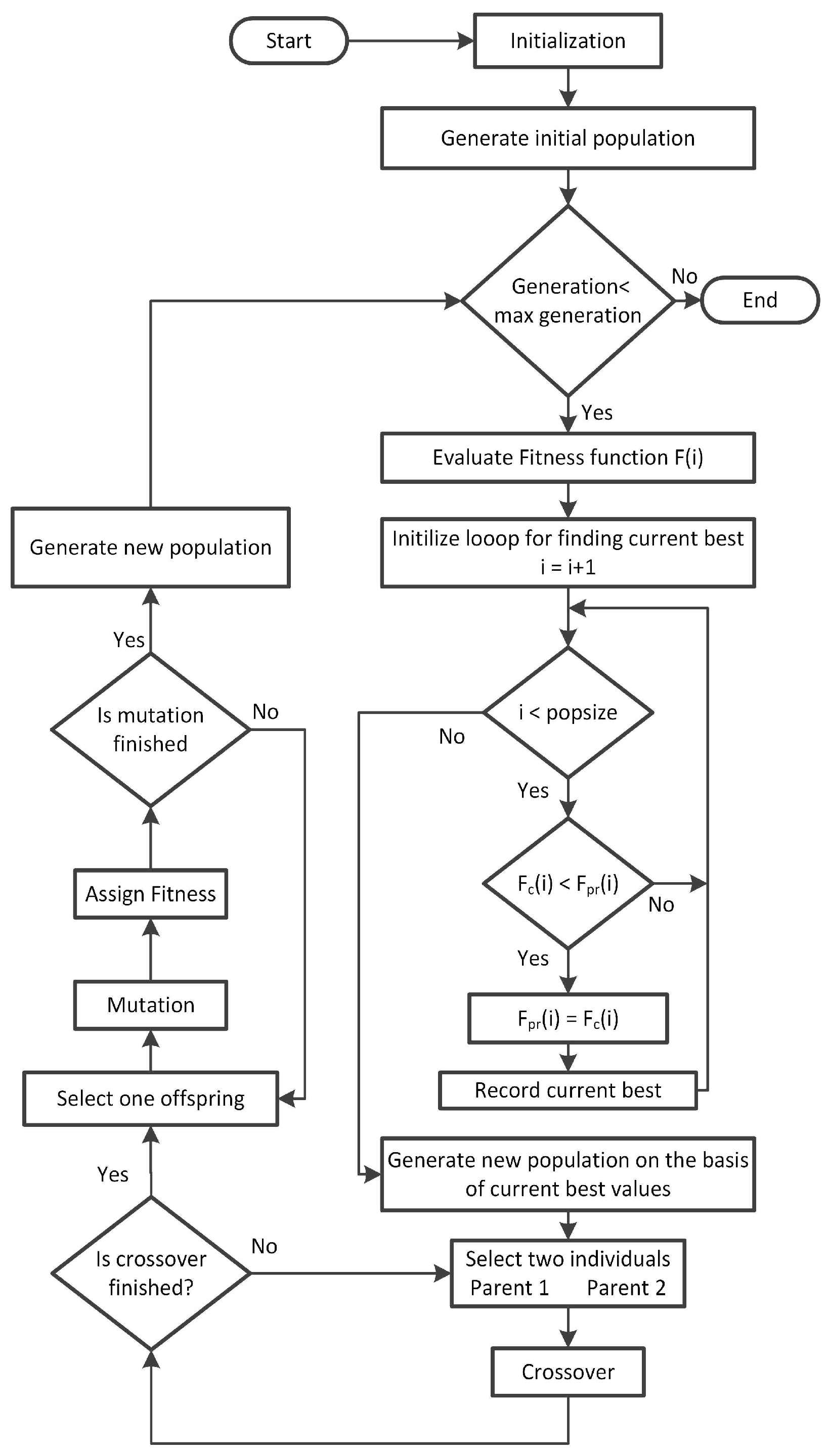
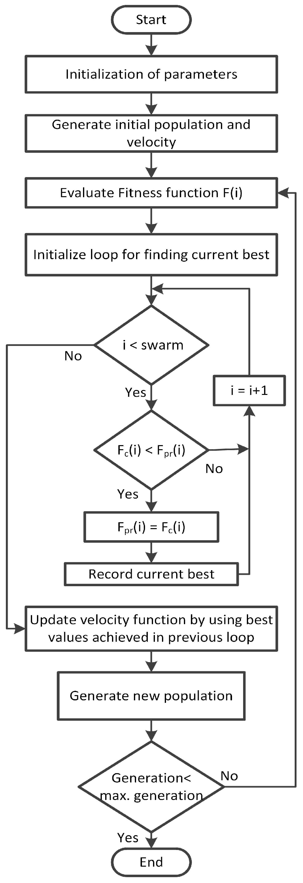
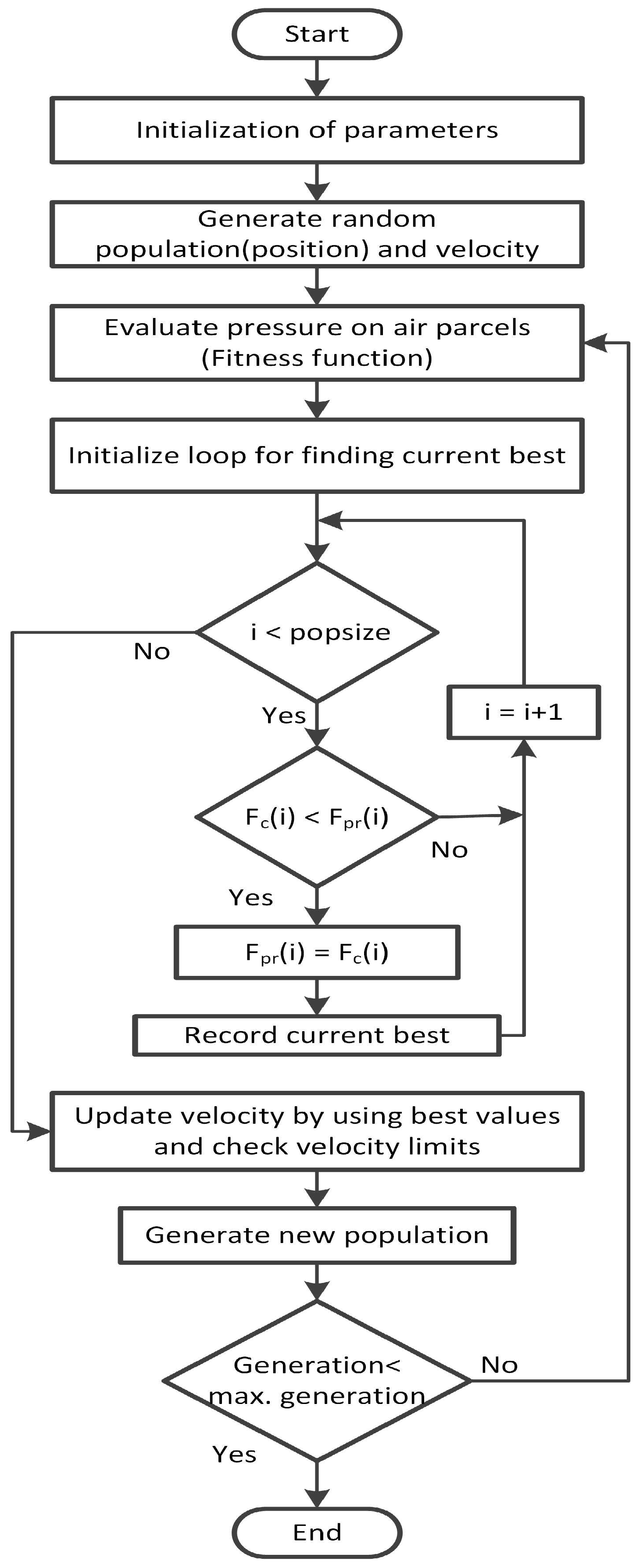
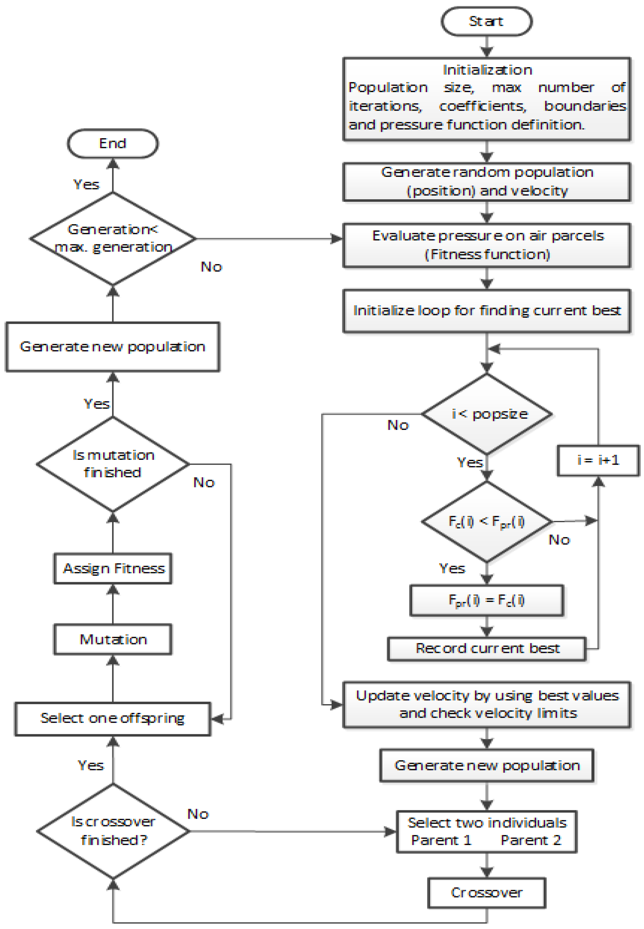
In this paper, we present the demand-side management of a residential household by scheduling that is based on heuristic techniques, which are implemented on an EMCU. The house is equipped with PV units, an ESS, and a set of electrical appliances that consume electrical energy from PV units and utility on the basis of electricity generation from PV units and prices. The household energy consumption behavior is optimized using heuristic techniques in order to reduce the electricity cost and PAR. Moreover, we develop the genetic wind-driven optimization (GWDO) algorithm, which is a hybrid of genetic algorithm (GA) and wind-driven optimization (WDO) algorithm, for load scheduling under a combined RTP and inclined block rate (IBR) environment to reduce electricity cost and PAR. To validate the performance of our proposed GWDO algorithm, simulations are carried out and results are compared with GA, binary particle swarm optimization (BPSO), WDO, and unscheduled electricity consumption in terms of electricity cost and PAR. It has been observed on the basis of comparison that our proposed scheme outperforms its counter parts.

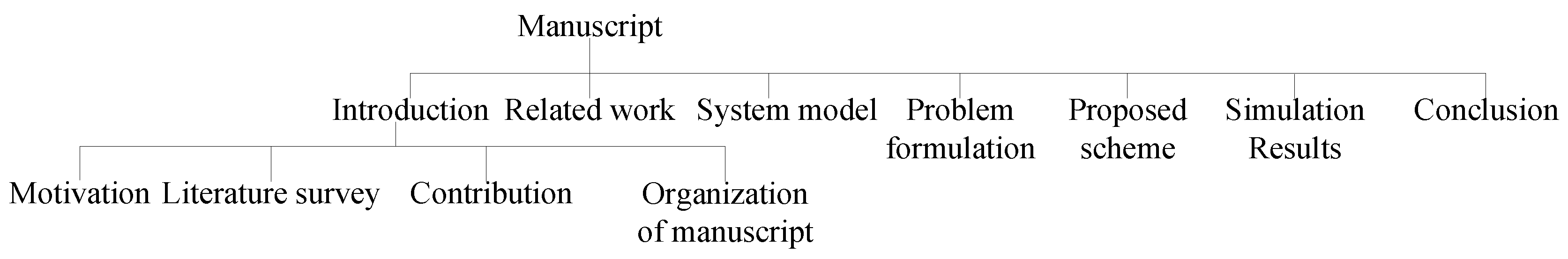
The rest of the paper is organized as shown in Figure 2. Related work is presented in Section 2. In Section 3, the system model is introduced. The problem formulation is discussed in Section 4. The proposed scheme is presented in Section 5. Section 6 includes simulation and discussion, and Section 7 concludes the paper. Finally, nomenclature used in the manuscript is given in Nomenclature.

2. Related Work

In order to optimally cope with the gap between demand and supply, numerous techniques and RESs integration are addressed in the literature. Authors in [15] presented demand-side energy consumption scheduling in the presence of PAR constraint and users preference in order to reduce the cost. Moreover, they introduce multi-objective optimization techniques which minimize the cost and inconvenience posed to users. They use a distributed algorithm to solve initial and multi-objective optimization problems. However, RESs integration is not addressed by the authors.

The authors implemented electricity storage and appliance scheduling schemes in [5] for the residential sector in order to reduce electricity costs. The storage system allows consumers to purchase electricity at off-peak times and satisfy their demand through storage during on-peak times. A day-ahead pricing scheme is used for electricity pricing. However, the uncoordinated charging and discharging of batteries results in discomfort for users. The authors in [6] proposed a smart home energy management system for the joint scheduling of electrical and thermal appliances. The controller receives price information and environment data in order to optimally schedule appliances to reduce cost. However, the authors achieved an economical solution at the cost of users’ comfort. The authors used intelligent decision support systems under a generic and flexible cost model for load scheduling in [7] to reduce the peaks and enhance the power system efficiency. The use of a generic and flexible cost model for hourly pricing reduced electricity cost. However, the authors reduced the peaks and cost while user comfort was comprised. The authors in [8] proposed joint access and load scheduling under DR schemes in order to reduce cost. Authors formulated an optimization problem for the EMC, enabling it to compute the target power level for the home while incorporating the effects of price variations and local wind power uncertainty. However, PAR was increased while reducing the cost. Authors in [9] proposed a residential load control algorithm for demand-side management under a combined RTP and IBR pricing scheme in order to reduce the electricity bill and PAR. However, the authors reduced peaks in demand while user comfort was minimized. The authors presented prosumers demand-side management in order to encourage consumers not only to take part in generation but also in efficient load scheduling [10]. The smart scheduler schedules household appliances under utility and distributed generation to reduce electricity cost. However, peaks in consumption emerged while reducing electricity cost, which may damage the entire power system.

The authors proposed an optimal scheduling method in [16] for distributed generations, battery ESSs, tap transformer, and controllable loads for SG application. They used a BPSO technique to solve the optimization problem and proved by simulation that total system losses were minimized and battery ESS sizes were considerably reduced. However, the system objectives were achieved at cost system complexity. The authors in [11] proposed two market models in order to cope with the gap between demand and supply. In [12], authors proposed a novel appliances commitment algorithm to optimally schedule appliances under operational constraints and economical considerations in order to maximize comfort and reduce cost. However, peaks may emerge while reducing cost because most users start operation during off-peak timeslots. Demand curve smoothing by controlling the charging strategies of electric vehicles was described in [13]. The authors proposed demand-side management strategies in SG in order to reduce PAR and cost. Moreover, they also proposed two smart pricing game theoretic approaches in order to provide customer privacy and communication overhead [14]. In [17], the authors investigated an optimal power scheduling method for DR in home energy management system.They proposed a solution that optimally schedules a set of appliances to reduce electricity bill and alleviate PAR. They introduced EMS in a home area network (HAN) based on SG and combined RTP with IBR model for electricity pricing.They used GA for solving nonlinear optimization problems. The results show that the scheme efficiently reduced both electricity bill and PAR. However, the proposed scheme achieved its objectives at the cost of user comfort.

An efficient heuristic-based EMC is utilized with RESs for load scheduling in the SG [18]. For electricity pricing, a combination of ToU tariff and IBR are used. The problem of load scheduling is formulated using multiple knapsack. The heuristic-based EMC performs optimal load scheduling in order to reduce electricity cost, PAR, and maximize user comfort. However, the objectives are achieved at the cost of system complexity.

The authors in [19] proposed an optimized home energy management system in the SG for demand-side management. The load scheduling problem was formulated as a multiple knapsack problem. They proposed hybrid genetic particle swarm optimization for load scheduling in the presence of RESs and ESS in order to reduce electricity cost and PAR. The simulation results evidenced that the proposed algorithm with RESs and ESS efficiently reduced the electricity cost and PAR. However, while reducing electricity cost and PAR, the comfort of the users was compromised and solar irradiance and temperature were assumed day-ahead.

Home load management in the SG is presented in [20]. The authors proposed a decentralized framework using a DR program to modify residential consumers’ load in order to minimize payments, and preserve their comfort and privacy. The simulation results indicated that the proposed approach was beneficial for both energy service provider and consumer. However, peaks may emerge while reducing cost and preserving comfort and privacy.

The authors in [21] proposed load scheduling of the residential sector in the SG. Day-ahead pricing is used for electricity cost calculation. They used integer linear programming for the scheduling of time-flexible and power-flexible appliances in order to reduce the cost and maximize user comfort. However, the authors achieved these objectives at the cost of PAR. Heuristic-based home EMC for residential load scheduling is proposed in [22]. Authors formulate load scheduling using multiple knapsack, and use RTP as a reference signal for cost calculation. In addition, they proposed genetic BPSO for the optimal scheduling of residential load in order to reduce electricity bill and PAR. However, the electricity bill and PAR were reduced while user comfort was compromised. The authors proposed community architecture for the effective management of electricity sources, and proposed a scheduling algorithm for the optimal scheduling of electrical appliances [23]. They reduced the electricity cost and PAR by adopting combined true RTP and IBR between community controller and end users. However, they achieved these objectives at the cost of user comfort. The authors in [24] proposed smart homes energy management using customer preferences and dynamic pricing. They performed optimal load scheduling of thermostatically controlled, user-aware, elastic, inelastic, and regular appliances in order to reduce cost while persevering comfort. However, objectives were achieved at the cost of system complexity. The authors proposed the long-term load scheduling problem and load demand as a Markov decision process based on a learning algorithm in order to reduce the cost and PAR of aggregated load [25]. For collaborative distribution system operator and transmission system operator, optimal power flow implementation decentralized decision-making was used. Moreover, they proposed an algorithm based on analytical target cascading for multilevel hierarical optimization in complex engineering problems. For coordination, diagonal quadratic approximation and truncated quadratic approximation are presented in order to solve optimal power flow in parallel. For validation of the proposed system, a 6-bus and the IEEE 118-bus test systems were used [26]. Authors in [27] proposed a self-decision-making method for load management using a multi-agent system while considering distributed generation and demand response resources in order to reduce the peak load of a distribution network feeder. Authors in [28] focus on a decentralized DR framework for both utility and consumers to respond varying prices to adjust its demand or supply in order to reduce utility generation cost and consumers’ discomfort cost. A modified IEEE 14-bus was used for performance evaluation of the proposed framework.

In [29,30], a day-ahead forecasting method is proposed for PV power output estimation 24 h before. A day-ahead forecasting of PV generation is performed using two deterministic models and a hybrid method based on an artificial neural network. The hybrid artificial neural network achieves fast and accurate forecasting results as compared to the deterministic models [29]. The authors of [30] used a physical hybrid artificial neural network to perform day-ahead forecasting of PV power using different training and testing data. The related work is summarised in

Table 1. Summary of related work.

References	Techniques	Objectives	Limitations
Demand-side energy consumption scheduling in presence of peak to average ratio (PAR) constraint and users’ preference [15]	Distributed algorithm	Minimization of cost	renewable energy sources (RESs) integration are not addressed
Electricity storage and appliances scheduling schemes for residential sector [5]	energy management control (EMC) and day-ahead pricing	Electricity cost reduction	Uncoordinated charging and discharging of batteries results in discomfort
Smart home energy management system for joint scheduling of electrical and thermal appliances [6]	Heuristic-based EMC	Optimal scheduling of appliances and cost reduction	Achieved economical solution at cost of users’ comfort
Intelligent decision support systems under generic and flexible cost model for load scheduling [7]	Generic and flexible cost model	Peaks reduction and enhancement of the power system efficiency	Reduced the peaks and cost while user comfort was comprised
Joint access and load scheduling under DR schemes [8]	Markov chain and derive the steady-state distribution	Cost reduction	PAR is increased while reducing the cost
Residential load control algorithm for demand-side management [9]	Energy consumption scheduling algorithm	Reduction of electricity bill and PAR	Reduced peaks in demand while user comfort is minimized
Prosumers demand-side management [10]	Smart scheduler	Reduction of electricity cost	Peaks in consumption emerged while reducing electricity cost, which may damage the entire power system
Optimal scheduling method for distributed generations, battery ESS, tap transformer, and controllable loads [16]	Binary particle swarm optimization (BPSO)	Minimization of total system losses	Objectives are achieved at the cost of system complexity
Two market models in order to cope with the gap between demand and supply [11]	Distributed demand response (DR) algorithms	Minimization of cost	Higher communication overhead and computing complexity
Optimal scheduling of appliances under operational constraints and economical consideration [12]	Novel appliances commitment algorithm	Comfort maximization and cost reduction	Peaks may emerge while reducing cost
Demand curve smoothing by controlling the charging strategies of electric vehicles [13]	Decentralized algorithm	Minimization of the peak demand loads	User comfort is compromised while reducing peaks in demand
Optimal power scheduling method for DR in home energy management system [17]	Genetic algorithm (GA)	Electricity cost and PAR reduction	The complexity of the system increased due to the division of scheduling time horizon
An efficient heuristic-based EMC is utilized with RESs for load scheduling in the SG [18]	GA, BPSO, and ACO algorithms	Minimization of electricity cost, PAR, and maximization of user comfort	Complexity of the system is increased while achieving the desired objectives
An optimized home energy management system in the smart grid (SG) for demand-side management [19]	GA, wind-driven optimization (WDO), BPSO, and hybrid of GA and BPSO algorithms	Cost and PAR minimization	User comfort is compromised
Home load management in the SG [20]	Decentralized framework and proposed scheduling algorithm	Cost reduction, comfort, and privacy reservation	PAR is compromised while reducing desired objectives

.

3. System Model

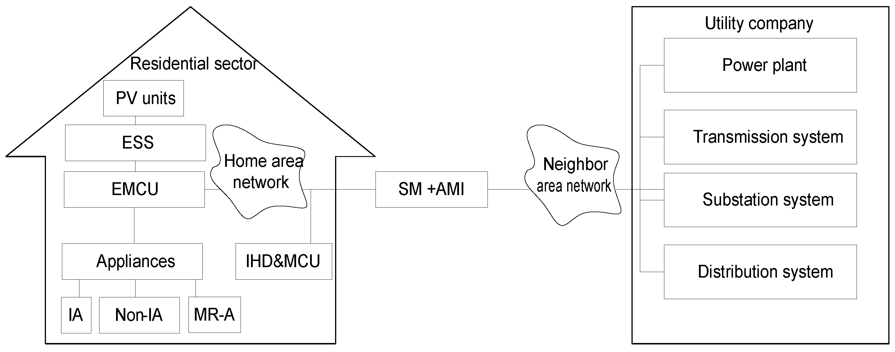
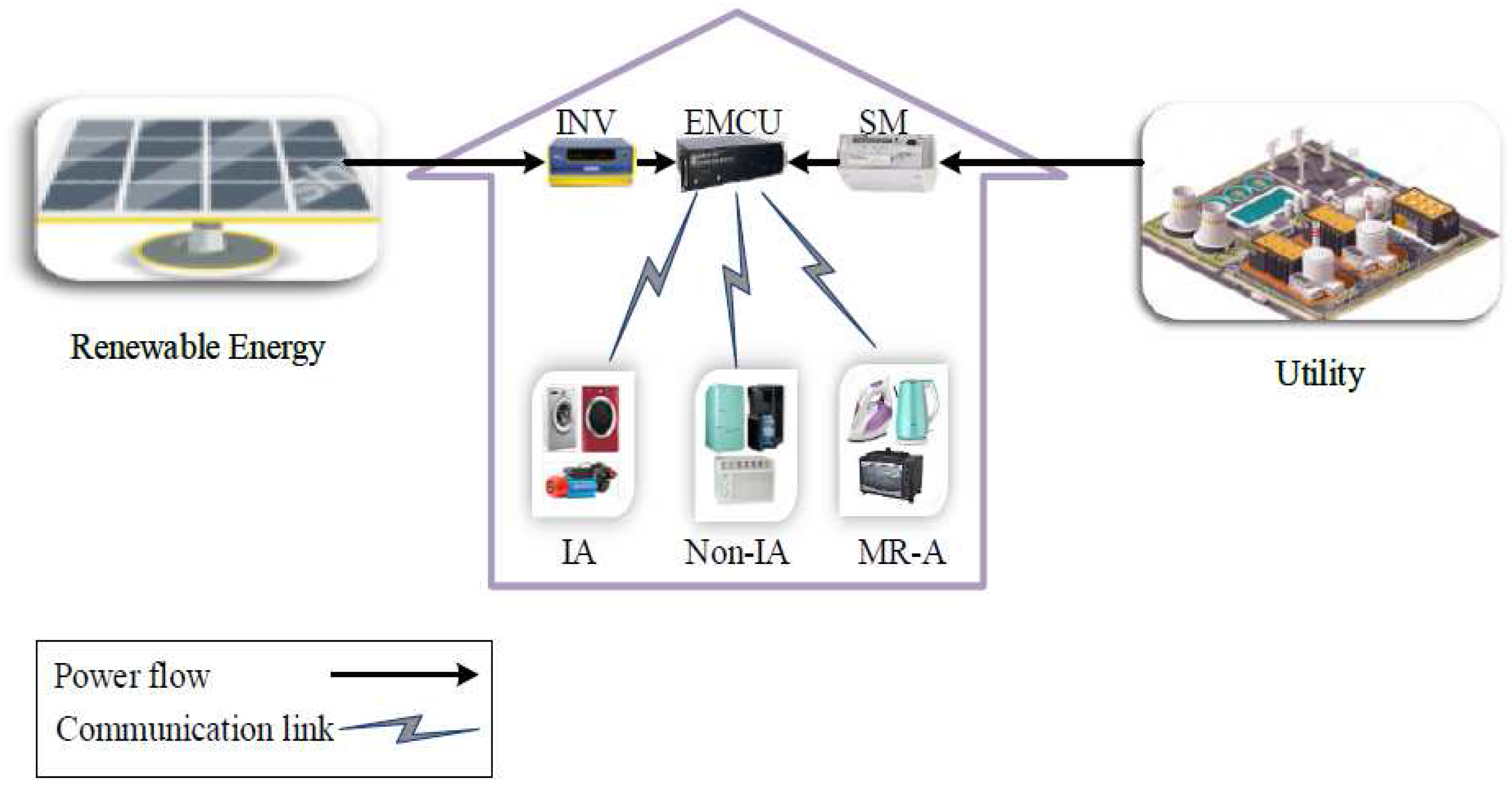
We consider a smart power system with a single utility company and serval users. Each user is equipped with RESs, such as rooftop PV units, as shown in Figure 3. The energy demands of users are fulfilled by their local RE generation and power imported from the utility company, as shown in Figure 4. Furthermore, the home energy management control system (HEMCS) comprises an EMCU, appliances, a smart meter (SM), in-home display and monitoring control unit (IHD & MCU), advanced metering infrastructure (AMI), and an inverter (INV). We assume that each home is equipped with a smart meter which is connected to the EMCU for load scheduling and adjusting energy consumption. We divided the scheduling time horizon into $T_h$ timeslots, where $T_h=\{1,2,3,\dots \dots ..,120\}$.

We classified appliances on the basis of their operation and demand requirements as IAs, Non-IAs, and must run appliances (MR-As). This classification is decided by users and can vary from time to time. The operation of IAs can be delayed or interrupted by the EMCU if required. In addition, IAs complete their operation in disjoint time intervals and the interruption of operation does not impact completion of the task. For example, washing machine, clothes dryer, and water motor are modeled as IAs.

Users may only require that washing machines must complete their task before the clothes dryer deadline or their water tank must be full of water before the deadline. Non-IAs cannot be interrupted, shifted, or shutdown during operation until completion; it is only possible to delay their operation. On the other hand, MR-As are refrigerator, air conditioner, and water cooler; these appliances are price inelastic because the refrigerator and dispenser need to be on at all times during the day. The appliances can either be in on status or off status.

Various pricing schemes are available for measuring the cost of consumers’ energy consumption, such as ToU, RTP, CPP, and critical peak rebates (CPRs). We consider the RTP method combined with IBR for electricity pricing because in the case of only RTP there is a possibility of building peaks during off-peak timeslots. $\chi \left(E_c^i\right)\left(t\right)$ represents the electricity price at each timeslot t as a function of the user’s power consumption. The combined pricing function $\chi \left(E_c^i\left(t\right)\right)$ is defined as:

$$\chi \left(E_c^i\left(t\right)\right)=\left\{\begin{array}{c}\phi \left(t\right)\mathrm{if}0\le E_c^i\left(t\right)\le E_{th}^i\hfill \\ b_t\mathrm{if}{E}_c^i\left(t\right)\ge E_{th}^i\hfill \end{array}\right.,$$

(1)

where $E_c^i\left(t\right)$ is the energy consumption at timeslot t, $\phi \left(t\right)$ is the real-time electricity price at timeslot t in a day, and $b_t$ is the price greater than $\phi \left(t\right)$ when $E_c^i\left(t\right)$ exceeds the threshold of IBR. The unit for measuring electricity cost is cents/kWh. At the beginning of the scheduling time horizon, each appliance i sends a request to the EMCU. The request specifies whether the appliance is an IA, a Non-IA, or an MR-A, as well as its operation start time and end time. The energy consumption of each appliance can be different at different timeslots due to changes in the amount of current being absorbed.

For each appliance i, we define the position $S_t^i=(r_t^i,w_t^i)$ of the appliance at timeslot t, where $r_t^i$ is the remaining operation timeslots of appliance i, and $w_t^i$ is the waiting timeslots for which appliance i must wait. We define $X_t=\{0,1\}$ as an indicator, indicating the status of the appliance—whether appliance i is in on state $(X_t=1)$ or in off state $(X_t=0)$. The position of appliances at the next timeslot $t+1$, $S_{t+1}^i$ can be found from their current position $S_t^i$, their type, and their status $X_t$.

For an IA, we can delay and interrupt its operation if required. The initial and next timeslot positions are demonstrated as

$$S_t^i=(T_o^i,\beta -\alpha +T_o^i+1),$$

(2)

$$\begin{array}{c}{S}_{t+1}^i=\left\{\begin{array}{c}{r}_t^i,w_t^i-1\mathrm{if}{X}_t=0,w_t^i\ge 1\hfill \\ r_t^i-1,w_t^i\mathrm{if}{X}_t=1,r_t^i\ge 1\hfill \end{array}\right..\hfill \end{array}$$

(3)

A Non-IA can only tolerate delay, and it is not possible to interrupt during operation until completion once it starts operation. The initial and next timeslot positions are demonstrated as:

$$S_t^i=(T_{o,}^i\beta -\alpha +T_{o,}^i+1),$$

(4)

$$\begin{array}{c}{S}_{t+1}^i=\left\{\begin{array}{c}{r}_t^i,w_t^i-1\mathrm{if}{X}_t=0,w_t^i\ge 1\hfill \\ r_t^i-1,0\mathrm{if}{X}_t=1,r_t^i\ge 1\hfill \end{array}\right..\hfill \end{array}$$

(5)

MR-As need to be on at all times during the day. For MR-As, the initial and next timeslot positions evolve as:

$$S_t^i=\left(T_{o,}^{i}0\right),$$

(6)

$$\begin{array}{c}{S}_{t+1}^i=\left\{\begin{array}{c}{r}_t^i,0\mathrm{if}{X}_t=1,r_t^i\ge 1\hfill \\ 0,0\mathrm{otherwise}\hfill \end{array}\right..\hfill \end{array}$$

(7)

Various types of RERs are available, such as, solar, wind, tidal, geothermal, biomass, and biogas energies. However, among the various types of RERs, solar is the most abundant, free of cost, and available everywhere to every one. According to [2], the Earth receives 174,000 terawatts (TW) of incoming solar radiation at the upper atmosphere. Approximately 30% is reflected back to space, while the rest is absorbed by clouds, oceans, and land masses. Most of the world’s population lives in areas with insolation levels of 150–300 W/m${}^2$ or 3.5–7.0 kWh/m${}^2$ per day. To take the benefit from solar energy, we integrate rooftop PV units with households to optimally schedule household appliances in order to reduce electricity cost, PAR, and carbon emission. The output power of PV units is calculated as [31]:

$$E^{PV}\left(t\right)={\eta }^{PV}.A^{PV}.I_r\left(t\right).(1-0.005(T^a\left(t\right)-25))\forall t,$$

(8)

where ${\eta }^{PV}$ is the percentage energy efficiency of the PV unit, $A^{PV}$ is the area of PV units in (m${}^2$), $Ir\left(t\right)$ is the solar irradiance (kW/m${}^2$) at time t, 0.005 is temperature correction factor [32], the outdoor temperature (${}^{\circ }$C) at time t and 25 is standard room temperature (${}^{\circ }$C). The distribution of hourly sun irradiation usually complies with a bi-modal distribution that can be considered as a linear blend of two uni-modal distribution functions. The uni-modal distribution functions can be modeled by Weibull probability density function, as shown in Equation (9) [31]:

$$f\left(I_r\left(t\right)\right)=\zeta \left(\frac{{\alpha }_1}{{\beta }_1}\right){\left(\frac{I_r\left(t\right)}{{\beta }_1}\right)}^{({\alpha }_1-1)e^{{\left(\frac{I_r}{{\beta }_1}\right)}^{{\alpha }_1}}}+(1-\zeta )\left(\frac{{\alpha }_2}{{\beta }_2}\right){\left(\frac{I_r\left(t\right)}{{\beta }_2}\right)}^{({\alpha }_2-1)e^{{\left(\frac{I_r}{{\beta }_2}\right)}^{{\alpha }_2}}},0<I_r\left(t\right)<\infty$$

(9)

where $\zeta$ is weighted factor, ${\alpha }_1$ and ${\alpha }_2$ are shape factors, and ${\beta }_1$ and ${\beta }_2$ are scale factors.

To cope with the gap between demand and supply, we assume that each user is equipped with PV units and an ESS. If the harvested energy is surplus or off peak hours, the energy is stored in the ESS. If the harvested energy is deficient, then all harvested energy is used to serve the load. The energy stored in the ESS is calculated by the following formula [31]:

$$E^{ESS}\left(t\right)=E^{ESS}(t-1)+\kappa .{\eta }^{ESS}.E{P}^{Ch}\left(t\right)-\frac{\kappa .E{P}^{Dch}\left(t\right)}{{\eta }^{ESS}},$$

(10)

where $E^{ESS}\left(t\right)$ is the stored energy at timeslot t while taking into account energy charged, discharged, and self discharging rate. ${\eta }^{ESS}$ is the efficiency of ESS, energy taken from rooftop PV units to charge ESS is $E{P}^{Ch}\left(t\right)$, and $E{P}^{Dch}\left(t\right)$ is the energy discharged from ESS to serve the load at timeslot t.

$$E{P}^{Ch}\left(t\right)\le E{P}_{UB}^{Ch},$$

(11)

$$E{P}^{Dch}\left(t\right)\le E{P}_{LB}^{Dch},$$

(12)

$$E^{ESS}\left(t\right)\le {E^{ESS\_}}_{UB}^{Ch},$$

(13)

where $E{P}_{UB}^{Ch}$ is the upper limit of charging ESS, $E{P}_{LB}^{Dch}$ is the lower limit of discharge, and ${E^{ESS\_}}_{UB}^{Ch}$ is the upper limit of the stored energy.

4. Problem Formulation

In demand-side management, residential load scheduling and the alignment of the stochastic demand under the utility and rooftop PV units are challenging tasks. Different techniques have been proposed in the literature addressing load scheduling for household energy management. For example, a GA-based DR scheme is presented in [17] for appliance scheduling to minimize the electricity bill and PAR. A smart scheduler algorithm is proposed for autonomous load scheduling under a ToU pricing tariff in order to increase the household revenue [10]. The load scheduling is performed via an energy consumption scheduling algorithm while considering load uncertainty in order to reduce PAR and payoff. However, peaks may emerge and user comfort may be compromised while reducing electricity cost. We proposed a GWDO algorithm for the load scheduling of a home having three types of appliances—IA, Non-IA, and MR-A—in order to reduce electricity cost and PAR. The reduction of PAR is beneficial for both consumers and utility because it reduces the number of peak power plants. To perform optimal residential load scheduling in the aforementioned technique, the scheduling period of one hour is divided into five timeslots; in other words, the time resolution is 12 min and one day has 120 timeslots. The resolution is set to be 12-min because it is short enough as a time unit for the operation intervals of all the household appliances, and it is much more convenient to solve the optimization problem. The formulation of energy consumption, electricity cost, PAR, and scheduling problem are described as follows.

4.1. Energy Consumption

We assume that the set of appliances are denoted by $A=\{A^{IA}\cup A^{Non-IA}\cup A^{MR-A}\}$, where $A^{IA}$ denotes a set of interruptible appliances, $A^{Non-IA}$ a set of non interruptible appliances, and $A^{MR-A}$ a set of must-run appliances. These appliances are scheduled over a time horizon of $T_h=\{1,2,3,\dots \dots ..,120\}$. The energy consumption of each appliance is given as:

$$E_c^i\left(t\right)=p_r^i\times X_t.$$

(14)

The aggregated energy consumption is calculated as:

$$E_T=\sum _{t=1}^{120}(\sum _{i=1}^n{E}_c^i\left(t\right)),$$

(15)

where $E_T$ denotes aggregated energy consumption.

4.2. Electricity Cost

Various pricing schemes are available for electricity cost calculation, such as, CPP, ToU tariff, and RTP; however, we adopted RTP. It is a midwest independent system operator (MISO) daily electricity price tariff taken from the FERC. The combined RTP and IBR scheme is used because in case of only RTP there is a possibility of building peaks during Off-peak hours that may damage the entire power system. The electricity cost is calculated as:

$$C_T=\sum _{t=1}^{120}\left(\sum _{i=1}^n{E}_c^i\left(t\right)\times \phi \left(t\right)\right),$$

(16)

where $C_T$ is the total cost and $\phi \left(t\right)$ is the RTP. The electricity cost after taking into account RESs and ESS is calculated as:

$$C_T=\sum _{t=1}^{120}\left(\sum _{i=1}^n{E}_c^i\left(t\right)-E^{PV}\left(t\right)-E^{ESS}\left(t\right)\right)\times \phi \left(t\right).$$

(17)

4.3. PAR

PAR is defined as the ratio of peak load to the average load consumed over the scheduling time horizon. PAR tells us about the energy consumption behavior and utility peak plants; it is beneficial for both utility and consumers. The PAR is calculated as follows:

$$\mathrm{Peak}=\max \left(E_c^i\left(t\right)\right),$$

(18)

$$\mathrm{Average}=\frac{1}{120}\sum _{t=1}^{120}(\sum _{i=1}^n{E}_c^i\left(t\right)),$$

(19)

$$\mathrm{PAR}=\frac{\mathrm{Peak}}{\mathrm{Average}}.$$

(20)

4.4. Scheduling Problem Formulation

The problem is formulated as a minimization problem because in load scheduling our main objectives are to reduce the electricity cost and PAR.

$$\min \left(\sum _{t=1}^{120}\left(\sum _{i=1}^n{E}_c^i\left(t\right)-E^{PV}\left(t\right)-E^{ESS}\left(t\right)\right)\times \phi \left(t\right)\right)+\min \left(\mathrm{PAR}\right),$$

(21)

subjected to:

$$E_T\le Capacity+E^{PV}\left(t\right)+E^{ESS}\left(t\right),$$

(21a)

$$\sum _{i\in A}{E}_T^{\mathrm{unsch}}=\sum _{i\in A}{E}_T^{\mathrm{sch}},$$

(21b)

$$\sum _{i\in A}{T}_o^{i-\mathrm{unsch}}=\sum _{i\in A}{T}_o^{i-\mathrm{sch}},$$

(21c)

$$X_t^{\mathrm{unsch}}\ne X_t^{\mathrm{sch}}.$$

(21d)

The constraint (21a) ensures that energy consumption must be under the capacity of utility and rooftop PV units. For fair comparison, constraints (21b) and (21c) ensure that the energy consumption and operation timeslots of unscheduled load must be equal to the scheduled load. Appliances’ proper scheduling are conformed from constraint (21d).

5. Proposed Scheme

The appliances are scheduled using GA, BPSO, WDO, and our proposed algorithm GWDO. The detailed description of these algorithms are as follows.

5.1. GA

GA is an optimization algorithm inspired from the genetic process of living organisms. The genetic chromosomes of GA represent the on/off status of appliances, and the length of chromosomes shows the number of appliances to be scheduled. Parameters of GA are initialized as shown in

Table 2. Parameters of GA.

Parameters	Values
Population size	100
n	9
Number of iterations	100
$P_c$	0.9
$P_m$	0.1

. First the population is randomly generated and fitness is evaluated according to our objective function. Then, after fitness evaluation a new population is generated by applying the crossover and mutation steps of the GA. A new population is generated at each iteration through crossover and mutation. In crossover, step two parents are selected to create new offspring. To avoid repetition and create randomness in the results, we use mutation. After crossover and mutation, again a population is generated and fitness is evaluated. Current results after fitness evaluation are compared to previous results in order to achieve the global optimal solution. The flow chart of the GA algorithm is shown in Figure 5.

5.2. BPSO

PSO is a nature-inspired optimization technique that uses the swarm intelligence concept to effectively solve large-scale nonlinear optimization problems while analytical methods suffer from slow convergence and the curse of dimensionality. We use BPSO in this paper, which is a modified discrete domain form of PSO [33]. For example, birds flock in search of food. When the birds move in search of food, they have some specific position and velocity. The EMCU based on BPSO mainly depends on four factors: initial position, initial velocity, particle best position, and global best position among all particles. The parameters of BPSO are initialized as shown in

Table 3. Parameters of BPSO.

Parameters	Values
Swarm size	9
n	9
Number of iterations	100
$c_1$	2
$c_2$	2
$w_i$	2
$w_f$	0.4
$vmax$	4
$vmin$	−4

. In the next step an initial position matrix is generated randomly, and the position of each particle represents a candidate solution. The velocity is computed using the following formula:

$$\begin{array}{c}\hfill v_i=vmax\times 2\times (rand(swarm,n)-0.5).\end{array}$$

(22)

A position matrix is a solution matrix which shows the status of the appliance while velocity controls the population generation. The initially generated position matrix is evaluated by a fitness function (objective function). Best values on the basis of fitness function for the current iteration are defined, called “pbest”. A collection of “pbest” values from all iterations are evaluated by fitness function to find global best (gbest). These gbest values are the status of appliances on which cost and PAR are minimum for a particular timeslot. The velocity formula is very important, as it consists of the control parameters that change the convergence behaviour of a solution. These control parameters include inertia factor, acceleration coefficients, previous, and best position values. These parameters are carefully selected as shown in Table 3.

Values of velocity are in real numbers, so they are converted into a binary state to obtain the status of each appliance. To convert into binary, sigmoid $\left(Sig\right)$ function is used, which is defined as:

$$Sig(j,i)=\frac{1}{1+e^{-v_{new}}}.$$

(23)

By applying Equation (23), the position matrix is updated as follows:

$$\left\{\begin{array}{c}{x}_{new}=1ifrand\left(1\right)\le Sig(j,i)\hfill \\ x_{new}=0ifrand\left(1\right)>Sig(j,i)\hfill \end{array}\right..$$

(24)

Fitness is evaluated on a new position; this process continues until the stopping criteria are fulfilled. At the end of this process, we get “gbest” values which are the optimum solution for the scheduling of our appliances. Moreover, the working step-by-step procedure of BPSO is described in Figure 6.

5.3. WDO

WDO is a nature-inspired optimization technique based on the atmospheric motion of wind. When the wind blows, it equalizes the horizontal imbalances. In this algorithm, we consider small air parcels as a candidate solution that are moving in N-dimensional space which experience different types of force [34]. The parameters of WDO are initialized as shown in

Table 4. Parameters of WDO.

Parameters	Values
Population size	20
n	9
Number of iterations	100
$RT$	3
g	0.2
$\alpha$	0.4
$dimMin$	−5
$dimMax$	5
$vmax$	0.3
$vmin$	−0.3

, along with their values.

In the next step, an initial position matrix is generated randomly which shows the status of appliances. Similarly, the initial velocity is generated which is mathematically defined as

$$\begin{array}{c}\hfill v_i=vmax\times 2\times (rand(populationsize,n)-0.5).\end{array}$$

(25)

This initially generated position matrix is evaluated by fitness function (objective function) and the states of the appliances for a particular timeslot are achieved; then, the velocity function is updated. In WDO, the velocity function is different from BPSO. In this function, we consider four different forces as control parameters. These parameters include gravitational force, pressure gradient force, coriolis force, and frictional force. In [34], an equation is derived for updating velocity by using these control parameters. Here $posnew$ shows the current status of appliances. At each iteration velocity and position, values must be updated. Using Equation (26), the new position of the air parcel for each iteration is defined as:

$$x_{new}=x_{cur}+u_{new}\Delta t.$$

(26)

Here $\Delta t$ is step time which is equal to 1; velocity at each iteration must be bounded by its maximum and minimum values, which are defined as:

$$u_{new}=\left\{\begin{array}{c}{u}_{max}if{u}_{new}>u_{max}\hfill \\ -u_{max}if{u}_{new}<u_{max}\hfill \end{array}\right..$$

(27)

After updating the velocity function again, a new “position” matrix is generated and evaluated. This process will continue until the stopping criteria are fulfilled. At the end of this process, we get “gbest” values which are the optimum solution for the scheduling of our appliances. Figure 7 shows the implementation of WDO.

5.4. GWDO

GWDO is our proposed algorithm which is a hybrid of GA and WDO. We chose these two algorithms because simulation results of GA and WDO show that GA is effective in PAR reduction and WDO is effective in cost reduction. So, we combined the features of GA and WDO so that the resulting algorithm should reduce both cost and PAR. The working procedure of GWDO consists of two phases, as shown in Figure 8. In the first phase we follow all the steps as in WDO, which are explained above. In the next phase genetic operations (crossover and mutation) are applied to gbest values of WDO. It improves results because crossover and mutation are applied on the best values instead of random values.

6. Simulations and Discussions

In this section, simulation results and discussions are presented in order to evaluate the performance of demand-side management under utility and RESs such as rooftop PV units. In our simulation settings, the scheduling time horizon of 24 h is divided into 120 timeslots; in other words, 1 h has five timeslots and one timeslot is 12 min. We compare our proposed algorithm GWDO with other heuristic algorithms (GA, BPSO, WDO) to validate the effectiveness of our proposed algorithm. Both our proposed algorithm GWDO and other heuristic algorithms (GA, BPSO, WDO) consider residential load scheduling under objective function, constraints, and rooftop PV units. We also compare our proposed algorithm GWDO with unscheduled, where EMCU is not deployed and residential load is not controlled. We consider a single home in the residential sector under utility and rooftop PV units having IA, Non-IA, and MR-A. A user in a single home has an average number of nine appliances. The description of the appliances are listed in

Table 5. Description of appliances.

Category	SA	OTS	Power Rating (kW)
Must-run appliances	Air conditioner	75	1.5
	Water cooler	70	1
	Refrigerator	60	0.5
Interruptible appliances	Washing machine	40	0.7
	Clothes dryer	40	2
	Water motor	36	0.8
Non-interruptible appliances	Electric kettle	20	1.5
	Electric iron	30	1.8
	Oven	25	2

; columns I and II show the appliance categories, column III shows the power rating of the appliances, and column IV shows the length of operation time of the corresponding appliance. The power consumption patterns of the appliances are known to the ECMU to allow proper scheduling of appliances. The length of operation of unscheduled appliances are the same as with scheduled appliances in order to have a fair comparison. For electricity pricing, we adopt the RTP method combined with IBR as described in Equation (1).

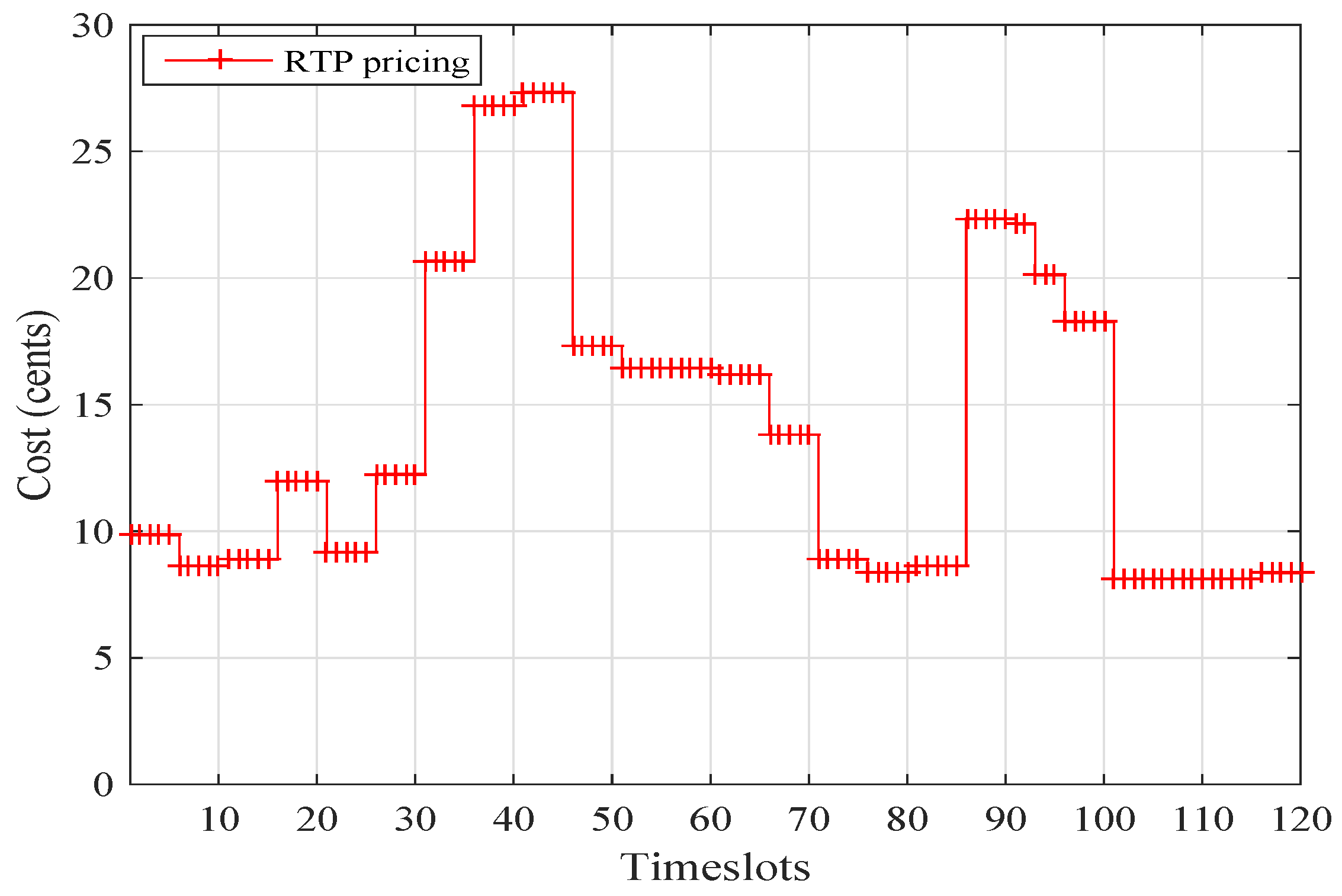
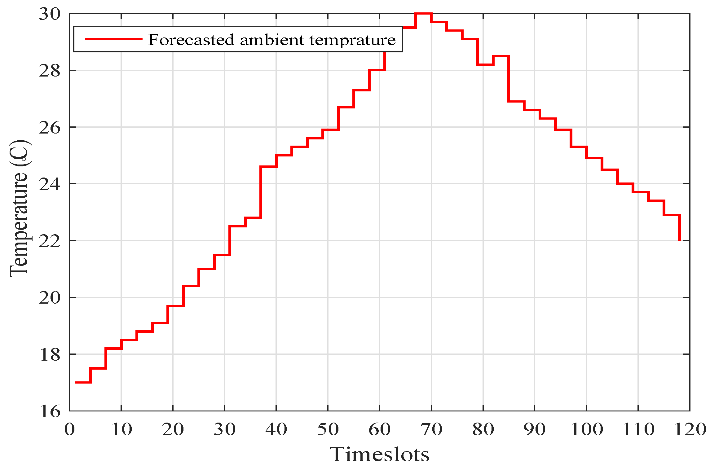
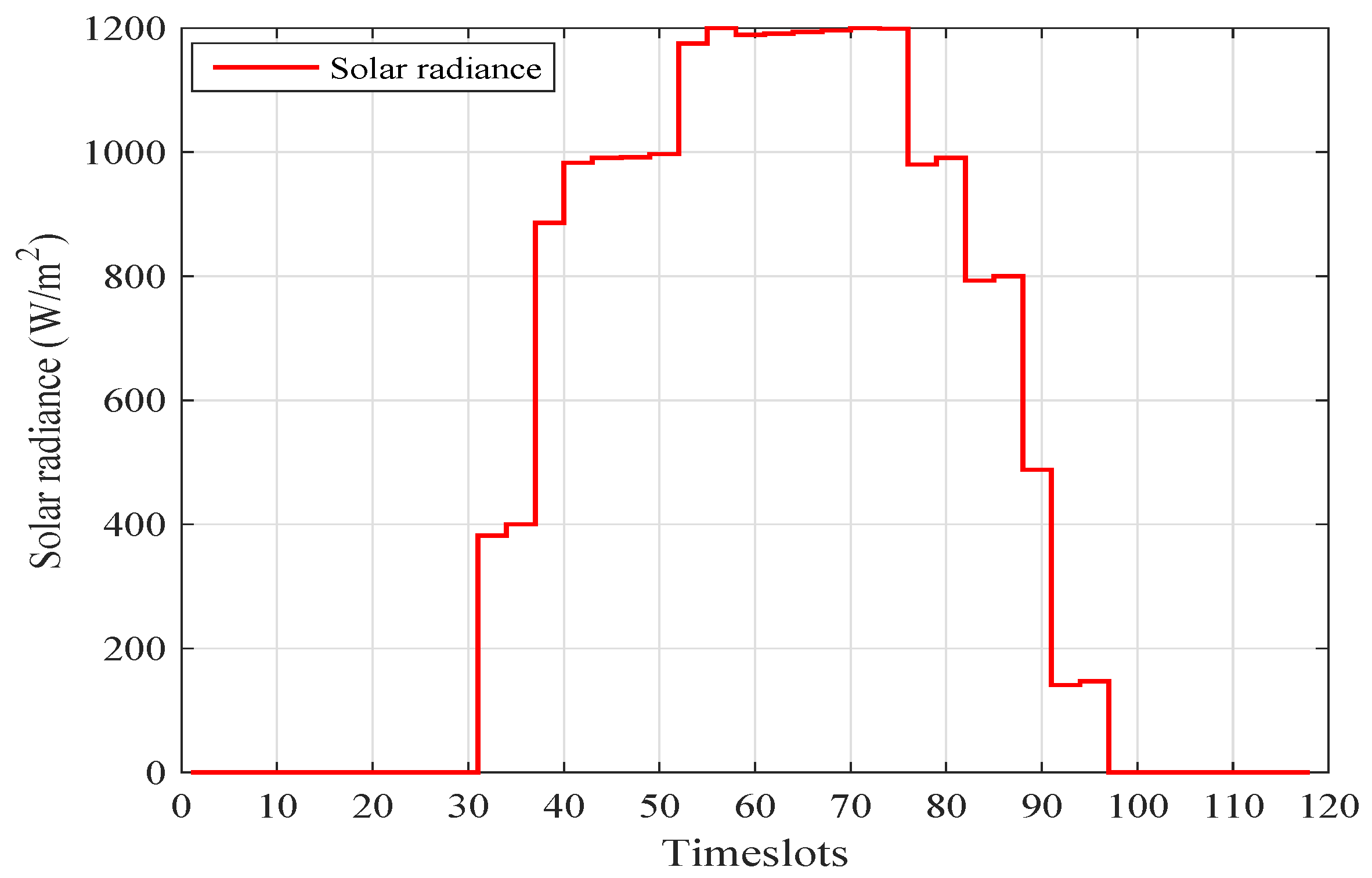
We assume that the utility company power is always available to support prosumers’ load. Moreover, the utility company gets the forecasted data of weather conditions, ambient temperature, and solar irradiance from the meteorological department, and broadcasts it to the prosumers. The RTP signal is the MISO daily electricity pricing tariff taken from FERC, as shown in Figure 9, and the normalized form of solar irradiance and temperature data obtained from METEONORM 6.1 for the Islamabad region of Pakistan is presented in Figure 10 and Figure 11.

The PV units generate electricity, depending on solar irradiance, ambient temperature, efficiency of PV units, and effective area of PV units. Ninety percent of the estimated PV generation in any timeslot of the scheduling time horizon is used to serve the load. The remaining 10% is left for uncertainty between the estimated and actual generation. Between 30–90% of PV units’ generation is used for charging the ESS only in the daytime. When the ESS is fully charged, it is utilized later during on-peak hours in order to reduce the electricity cost and PAR.

6.1. Feasible Region

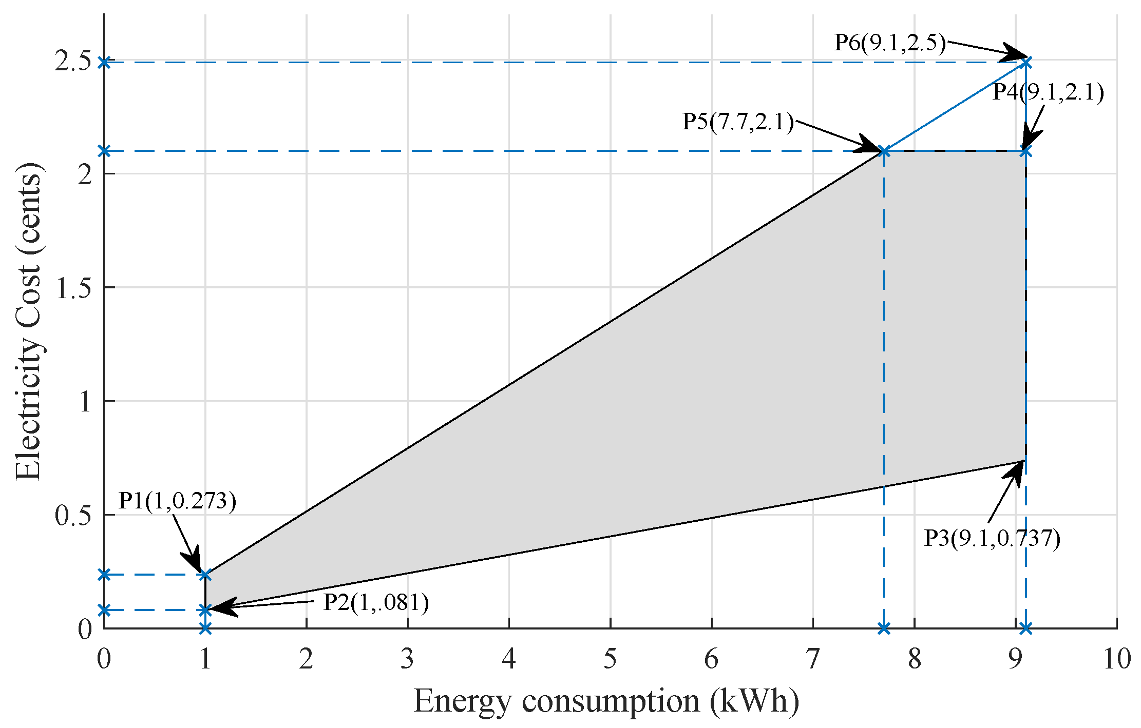
The feasible region is an area defined by a specific set of points in which the objective function satisfies the result. In our case, the objective function is to minimize cost and PAR by controlling energy consumption. So, our objective function is defined by Equation (21). To find the constraints of this objective function, we consider an RTP signal whose range is (0.081:0.2735) cents/kWh. So, we calculate four possible cases as:

$$\begin{array}{c}\mathrm{Min}\mathrm{load},\mathrm{Min}\mathrm{EP}:1\times 0.081=\mathrm{cents}0.081\hfill \\ \mathrm{Min}\mathrm{load},\mathrm{Max}\mathrm{EP}:1\times 0.273=\mathrm{cents}0.273\hfill \\ \mathrm{Max}\mathrm{load},\mathrm{Min}\mathrm{EP}:9.1\times 0.081=\mathrm{cents}0.737\hfill \\ \mathrm{Max}\mathrm{load},\mathrm{Max}\mathrm{EP}:9.1\times 0.2735=\mathrm{cents}2.488\hfill \end{array}$$

Additionally, the maximum cost of unscheduled load is 2.1 cents. Based upon these values, we define our constraints so that the cost of scheduled load should be less then unscheduled cost in each timeslot. Hence, constraints are defined as

$$0.081\mathrm{cents}<\mathrm{x}<2.1\mathrm{cents},$$

(28)

$$1kWh<y<9.1kWh,$$

(29)

where x represents cost and y represents energy consumption. Constraint (29) represents that the maximum unscheduled load in any timeslot can be 9.1 kWh, so scheduled load should be less than this load. Similarly, constraint (28) is that the maximum cost in each timeslot is 2.1 cents, so we schedule load such that cost should not be greater than 2.1 cents in any timeslot. In Figure 12, the total cost range is shown by the trapezium (P1 P3 P6 P2), while the shaded portion which is surrounded by P1, P2, P3, P4, and P5 is a feasible region.

6.2. Energy Consumption Behavior of Appliances

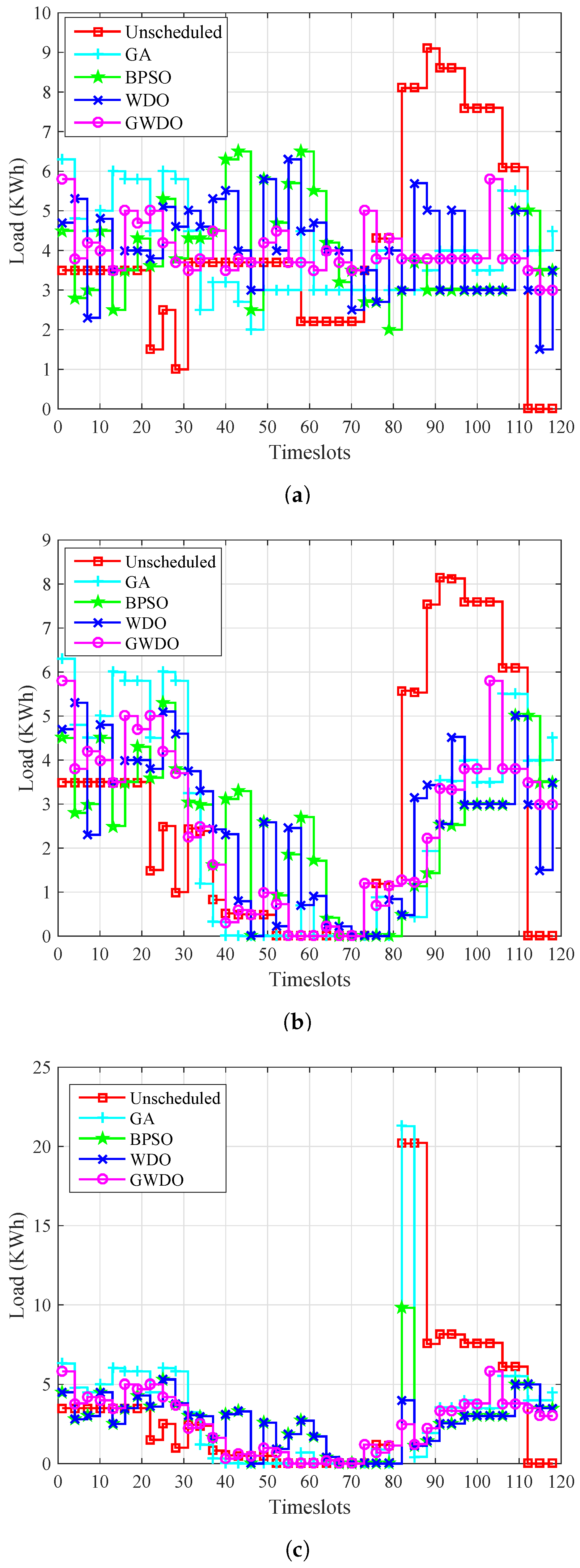
The energy consumption profile of scheduled (GA, BPSO, WDO, GWDO) and unscheduled load without RESs and ESS, with RESs, and with RESs and ESS is shown in Figure 13.

The load scheduled based on (GA, BPSO, WDO, GWDO) and unscheduled without RESs and ESS is shown in Figure 13a. The unscheduled load of users without RESs and ESS have consumption peaks of 9.1 kWh at timeslot 90, 8.90 kWh during timeslots 91 to 93, 8 kWh during timeslots 81 to 83, 7.8 kWh during timeslots 94 to 106, and 6 kWh during timeslots 107 to 111. The energy consumption of users in the unscheduled case without RESs and ESS is moderate other than these timeslots. The scheduled load based on GA of users have peak energy consumption of 6.1 kWh at timeslots 1 to 2, 6 kWh at timeslots 11 and 25. The GA scheduling of users have moderate energy consumption in the remaining timeslots. The percent decrement of peak power consumption in the case of GA as compared to unscheduled is 32.96%. The BPSO-based scheduling of users has peak energy consumption of 6.2 kWh at timeslot 42 and 59 and 6.1 kWh at timeslot 40 to 41. The load scheduled based on BPSO has moderate energy consumption in the remaining timeslots. The peak energy consumption of BPSO is 31.86% less than the unscheduled case. In the case of WDO-based scheduling, the peak energy consumption was 6.05 kWh at timeslot 59 and 5.8 kWh at timeslots 51 and 85. WDO-based scheduling has moderate energy consumption in the remaining timeslots. The percent decrement in peak power consumption in the case of WDO is 33.51% as compared to unscheduled.

Our proposed GWDO-based scheduling had a peak energy consumption of 5.9 kWh at timeslots 1, 2, and 106 and moderate energy consumption in the remaining timeslots. The percent decrement of GWDO is 35.16% as compared to unscheduled.

The GWDO outperforms unscheduled and other heuristic techniques (GA, BPSO, WDO) because GWDO has the most suitable, stable, and optimal load profile as compared to the other techniques, as is clear from Figure 13a.

The load scheduled based on (GA, BPSO, WDO) and unscheduled with RESs is shown in Figure 13b. The peak energy consumption of scheduled load based on GA, BPSO, WDO, GWDO, and unscheduled are 6.1 kWh at timeslot 1 to 2, 5.6 kWh at timeslots 28 to 29, 5.5 kWh at timeslots 6 to 7, 5.8 kWh at timeslots 1 and 103, and 8.1 kWh at timeslots 91 to 95, respectively. The percent decrement of heuristic techniques (GA, BPSO, WDO, GWDO) as compared to unscheduled are 24.69%, 30.86%, 32%, 28.39%, respectively. Our proposed scheme GWDO over all profile loads with RESs is better than the other heuristic techniques (GA, BPSO, WDO).

The unscheduled load and scheduled load based on (GA, BPSO, WDO, GWDO) with RESs and ESS is shown in Figure 13c. Our proposed scheme GWDO over all load profiles with RESs and ESS is best among the other heuristic techniques (GA, BPSO, WDO) and unscheduled load, as is clear from Figure 13c.

6.3. Electricity Cost per Timeslot Analysis

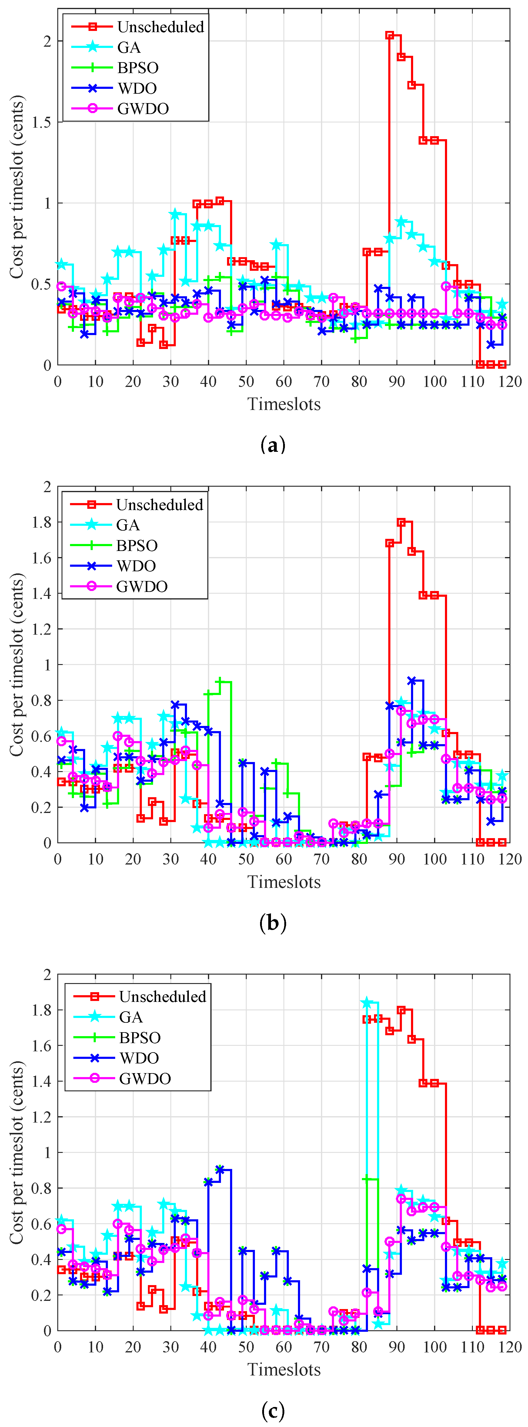
The electricity cost per time slot profile of scheduled load based on (GA, BPSO, WDO, GWDO) and unscheduled without RESs and ESS, with RESs, and with RESs and ESS are shown in Figure 14.

The electricity cost of scheduled load based on (GA, BPSO, WDO, GWDO) and unscheduled load without RESs and ESS is shown in Figure 14a. The maximum electricity cost per timeslot of scheduled load based on GA, BPSO, WDO, GWDO, and unscheduled load are 0.9 cents/kWh at timeslot 31, 0.6 cents/kWh at timeslots 43 and 58, 0.55 cents/kWh at timeslot 57, 49 cents/kWh at timeslots 1 and 103, and 2.1 cents/kWh at timeslots 88 and 89. As is clear from Figure 14a, our proposed scheme GWDO has the most stable and optimal electricity cost profile as compared to other heuristic algorithms and unscheduled load.

The electricity cost of scheduled load and unscheduled load with RESs is shown in Figure 14b. The maximum electricity cost of unscheduled load with RESs is 1.8 cents/kWh at timeslots 91 to 93, 1.7 cents/kWh at timeslots 89 to 91, 1.65 cents/kWh at timeslots 97 and 98, and 1.4 cents/kWh at timeslots 99 to 102 because the users do more activities in these timeslots, and therefore energy consumption in these timeslots is high, resulting in high electricity cost. GA-based scheduled load has a maximum electricity cost of 0.8 cents/kWh at timeslot 91, 0.7 cents/kWh at timeslots 16 to 21 and 29 to 31 because the energy consumption at these timeslots is maximum. GA has moderate energy consumption other than these timeslots, which results in less electricity cost as compared to the mentioned electricity cost. The BPSO-based scheduled load has a maximum electricity cost of 0.9 cents/kWh at timeslot 43, 0.85 cents/kWh at timeslot 41, and 0.7 cents/kWh at timeslots 35 and 36 due to the high energy consumption at these timeslots. The WDO-based scheduled load has a maximum electricity cost of 0.9 cents/kWh at timeslot 93 and 0.75 cents/kWh at timeslots 31, 32, 89, and 90 because in this scenario energy consumption is high in these timeslots. The electricity cost is moderate during timeslots other than those mentioned. Our proposed scheme GWDO is better than other heuristic techniques (GA, BPSO, WDO) in terms of electricity cost, as shown in Figure 14c.

The comparative analysis of scheduled load based on (GA, BPSO, WDO, GWDO) and unscheduled load with RESs and ESS in terms of electricity cost is shown in Figure 14c. The simulation results show that GWDO has the most suitable, stable, and optimal profile as compared to unscheduled load and other heuristic techniques (GA, BPSO, WDO) in terms of electricity cost.

6.4. Total Cost Analysis

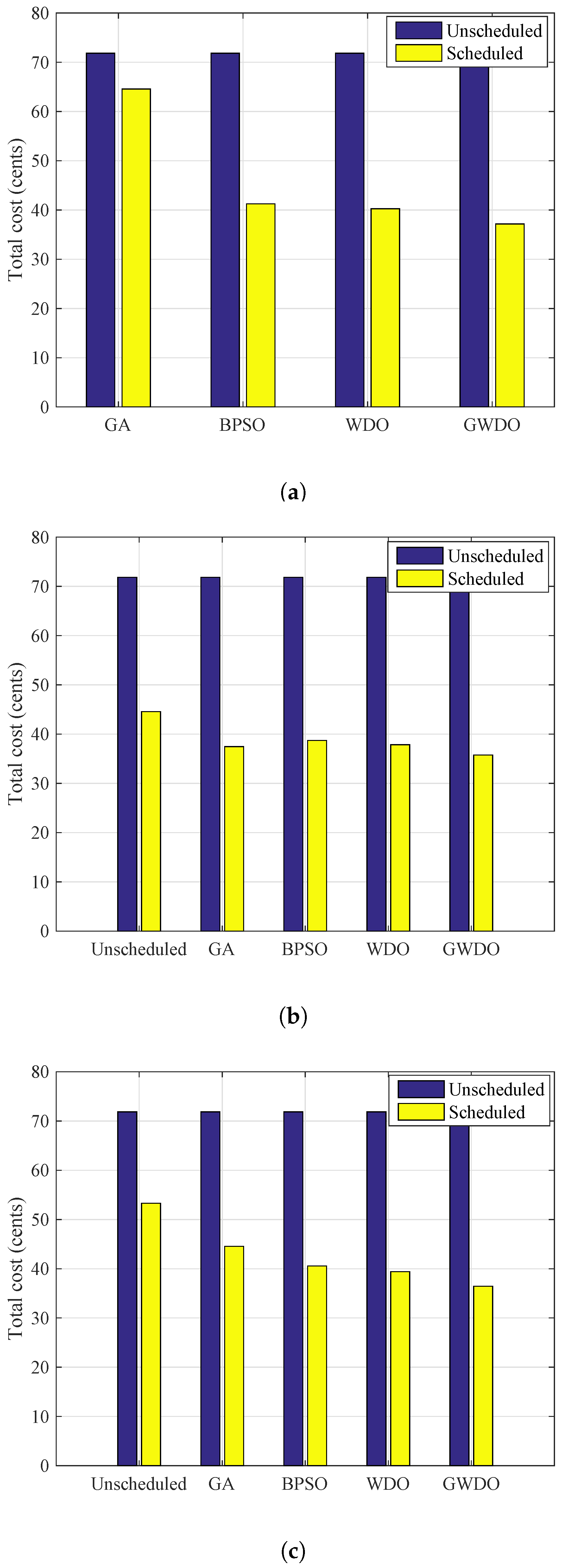
The comparison of the aggregated cost of scheduled load using (GA, BPSO, WDO, GWDO) and unscheduled load without RESs and ESS, with RESs, and with RESs and ESS is shown in Figure 15.

The aggregated cost analysis of scheduled load without RESs is shown in Figure 15a. The heuristic techniques GA, BPSO, WDO, and our proposed GWDO reduce the electricity cost by 4.2%, 15.49%, 18.3%, and 22.5%, respectively. The percent decrement in the case of our proposed GWDO is greater compared to unscheduled and scheduled load using heuristic techniques (GA, BPSO, WDO).

The aggregated cost analysis of scheduled load with RESs is shown in Figure 15b. The percent decrement of our proposed GWDO technique is 47.7% as compared to unscheduled because it employs the crossover and mutation steps of GA on best values rather than on random values. So, our scheme outperforms the other heuristic techniques GA, BPSO, and WDO.

The aggregated cost with RESs and ESS of scheduled load and unscheduled load is shown in Figure 15c. The percent decrement of our proposed scheme with the incorporation of RESs and ESS are greater than without RESs and with RESs. Therefore, our scheme is beneficial for consumers in order to reduce their cost.

6.5. PAR Analysis

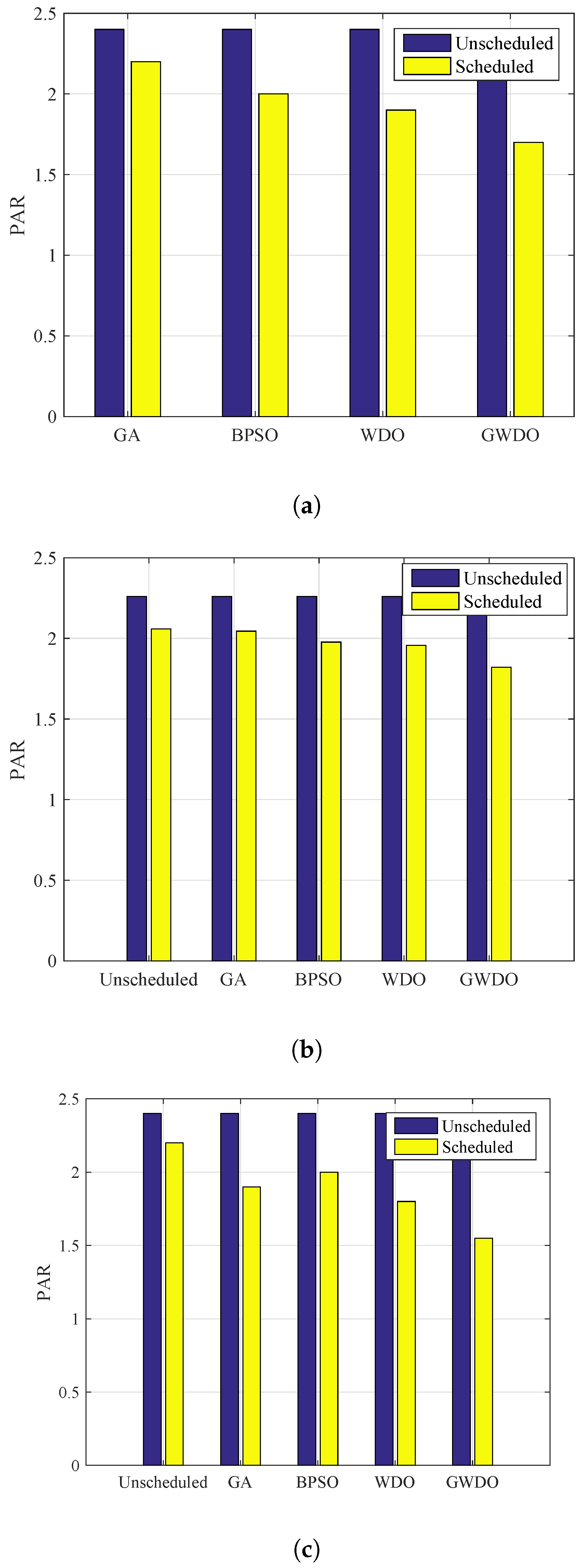
The PAR of the consumers’ load without RESs and ESS, with RESs, and with RESs and ESS is shown in Figure 16.

The PAR of scheduled load using (GA, BPSO, WDO, GWDO) and unscheduled without RESs and ESS is shown in Figure 16a. The EMCUs based on all these algorithms are designed to avoid the peaks, which results in reduction of the PAR. GA, BPSO, WDO, and GWDO reduce the PAR as compared to the unscheduled case by 8.3%, 16.5%, 20.8%, and 29.1%, respectively. The percent decrement of GWDO is greater than the other heuristic techniques, which ensures that our proposed scheme outperforms the other heuristic techniques. This reduction in PAR provides benefits to utility and consumers in terms of power system stability and electricity bill savings, respectively.

The PAR of scheduled load using (GA, BPSO, WDO, GWDO) and unscheduled with RESs is shown in Figure 16b. The simulation results show that with the incorporation of RESs our proposed algorithm GWDO reduces the PAR by 30% as compared to the unscheduled load case. Moreover, our proposed algorithm tackles the problem of peak formation and optimally shifts the load from on-peak timeslots to off-peak timeslots.

The PAR of scheduled load based on (GA, BPSO, WDO, GWDO) and unscheduled with RESs is shown in Figure 16c. Results show that the integration of RESs reduces the PAR by 30% and after incorporating the ESS as well, the PAR is reduced by 35.4%. This reduction in PAR not only enhances the stability and reliability of the power system, but also reduces the electricity bill of the consumers. The brief description of performance evaluation of existing and proposed algorithm in terms of electricity cost and PAR is summarized in

Table 6. Comparative analysis of existing and proposed techniques.

Techniques	Cost Reduction: Scenario 1	Cost Reduction: Scenario 2	Cost Reduction: Scenario 3	PAR Reduction: Scenario 1	PAR Reduction: Scenario 2	PAR Reduction: Scenario 3
GA	4.2%	11.6%	13.46%	8.3%	4.5%	17.39%
BPSO	15.49%	9.3%	21.5%	16.5%	11.36%	13.04%
WDO	18.3%	13.95%	25%	20.8%	13.6%	26.08%
GWDO	22.5%	47.7%	49.2%	29.1%	30.%	35.4%

.

7. Conclusions and Future Work

In this paper, we first introduce the system model for a residential household under utility and rooftop PV units, and then proposed the GWDO algorithm, which is a hybrid of GA and WDO, for electricity cost reduction using a combined RTP and IBR pricing scheme. In this regard, we considered three scenarios: (1) energy consumption from utility without RESs and ESS integration, (2) energy consumption from utility and from RESs, and (3) energy consumption from utility with RESs and ESS integration. The main idea is to encourage consumers to take part in RE generation and load scheduling to cope with the gap between demand and supply of electricity. To validate the performance of our proposed GWDO algorithm, simulations are carried out and results are compared with GA, BPSO, WDO, and unscheduled electricity consumption in terms of electricity cost and PAR reduction. Moreover, our proposed GWDO technique outperforms in terms of electricity cost and PAR reduction as compared to its counterparts. Furthermore, our proposed scheme reduced electricity cost and PAR by 22.5% and 29.1% in scenario 1, 47.7% and 30% in scenario 2, and 49.2% and 35.4% in scenario 3, as compared to unscheduled electricity consumption.

In the future, in addition to scheduling, load forecasting and power trading concept between the prosumers and the utility grid will be considered to cope with the gap between demand and supply to enhance the reliability of the power system.