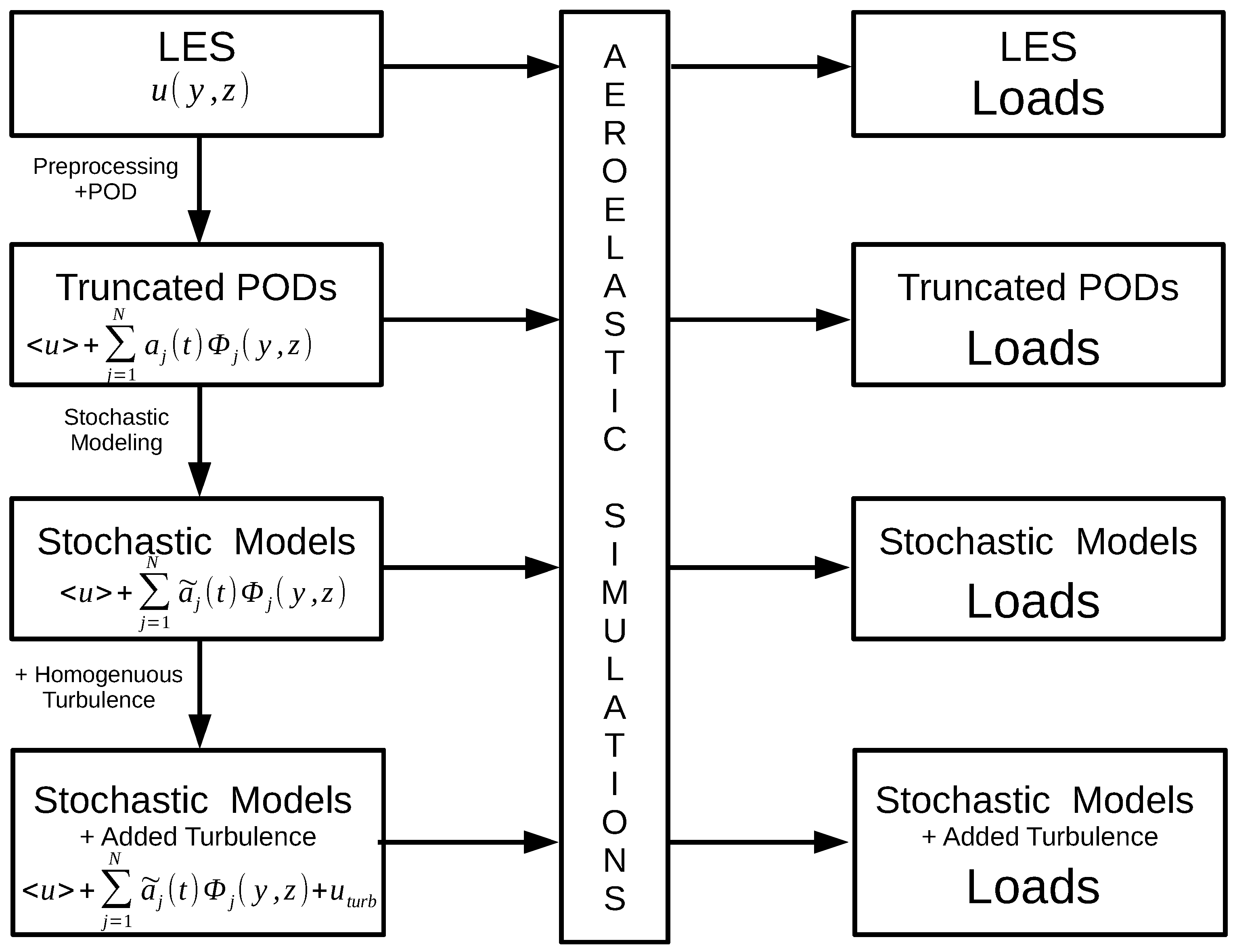
Stochastic Wake Modelling Based on POD Analysis

Abstract
1. Introduction
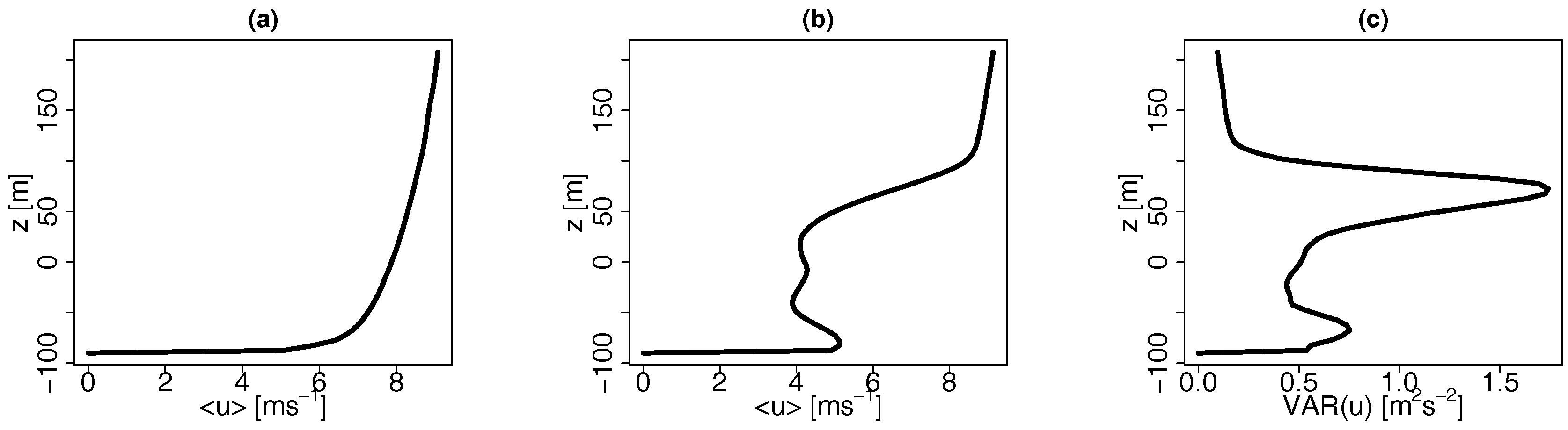
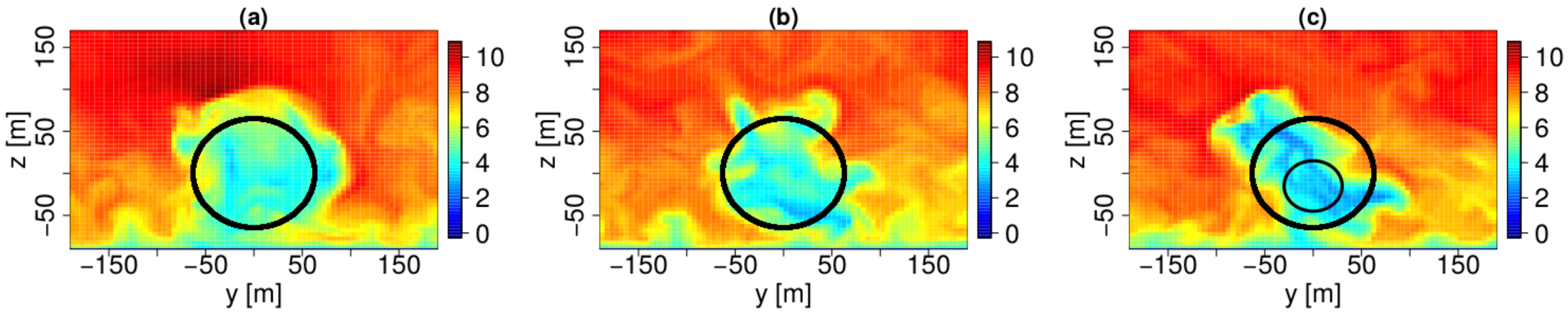
2. LES Simulations
3. Methods
3.1. Preprocessing
3.2. POD
3.3. Temporal Stochastic Modelling
3.3.1. Uncorrelated Model
3.3.2. OU-Based Model
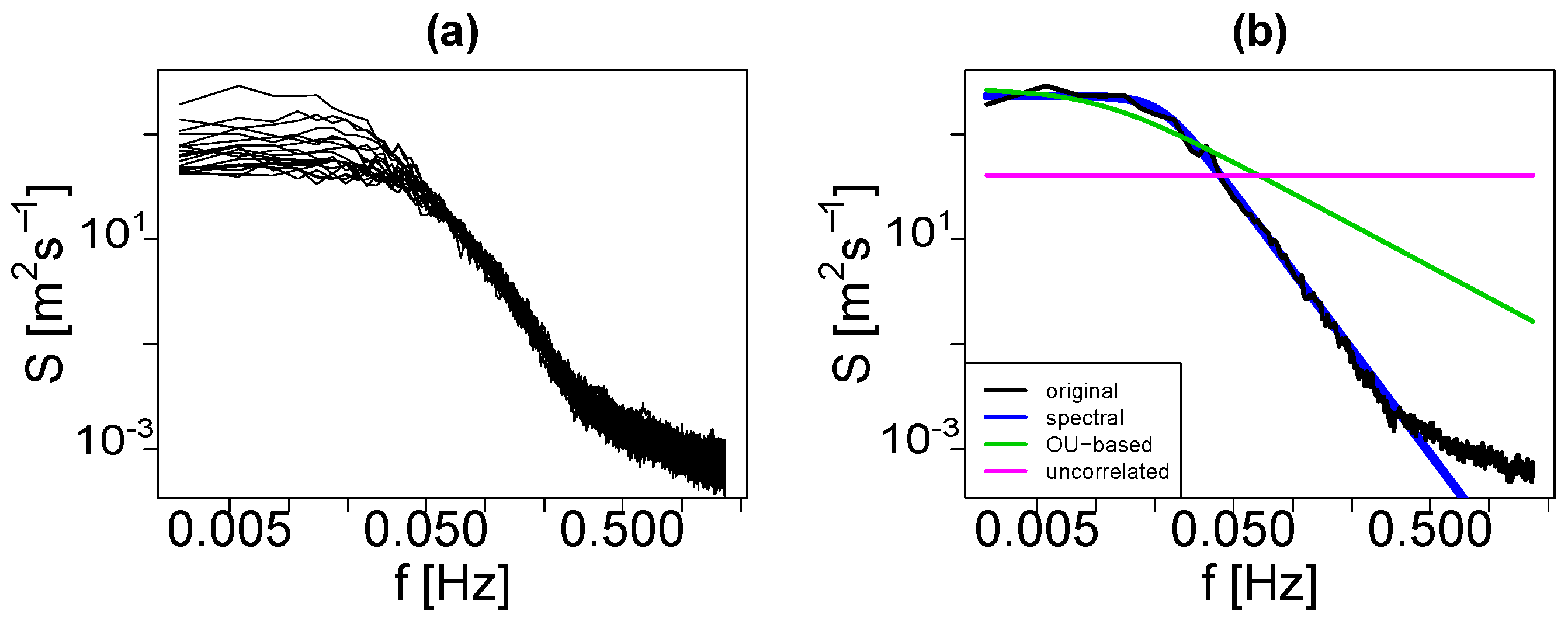
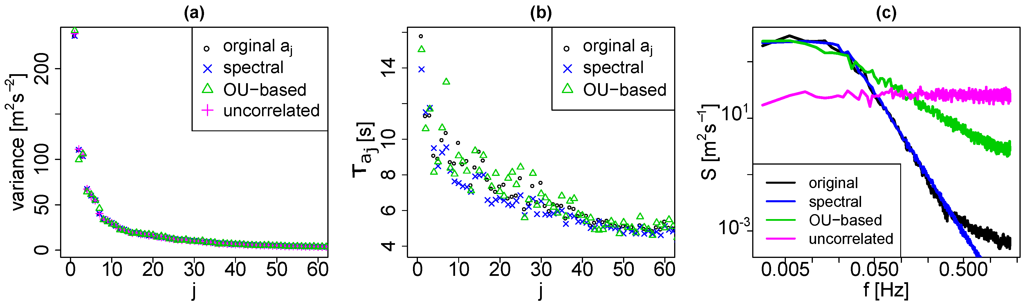
3.3.3. Spectral Mode
3.3.4. Comments on More Complex Models
3.4. A Spectral Surrogate in Three Dimensions
3.5. Aeroelastic Simulations and Model Verification
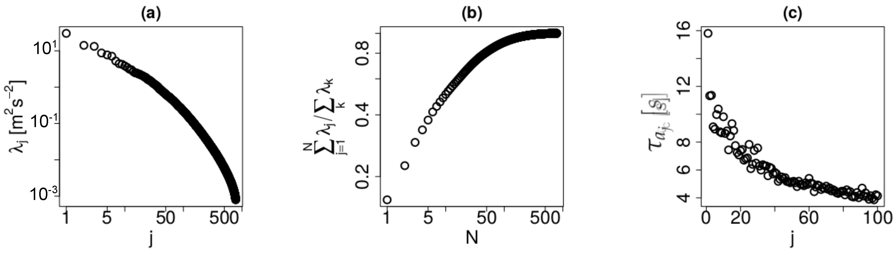
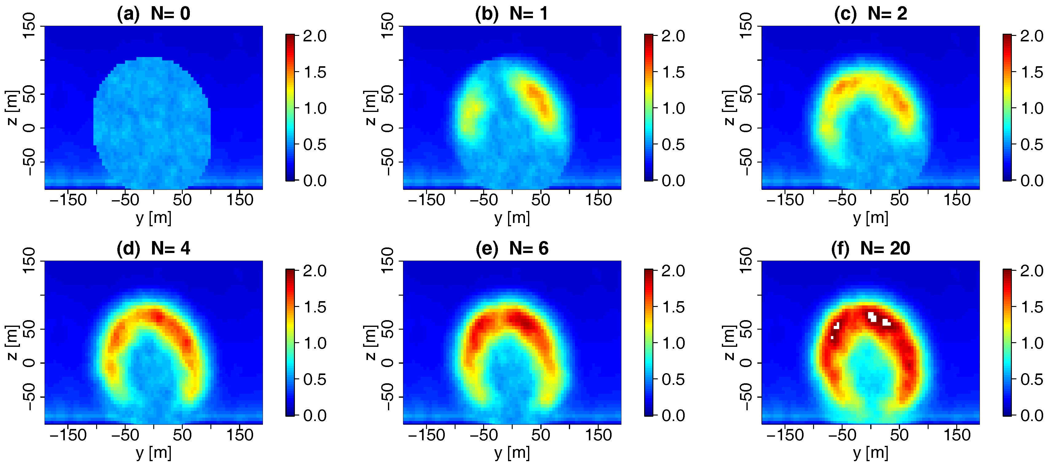
4. Truncated PODs
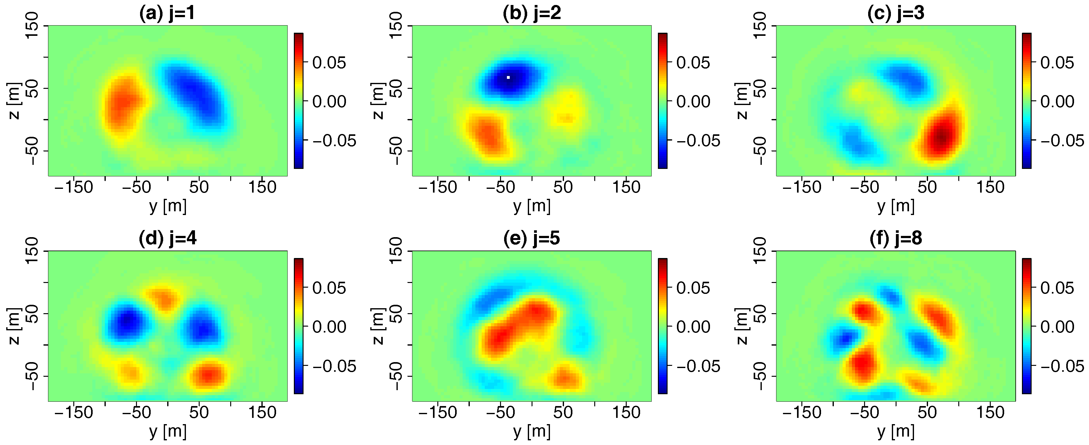
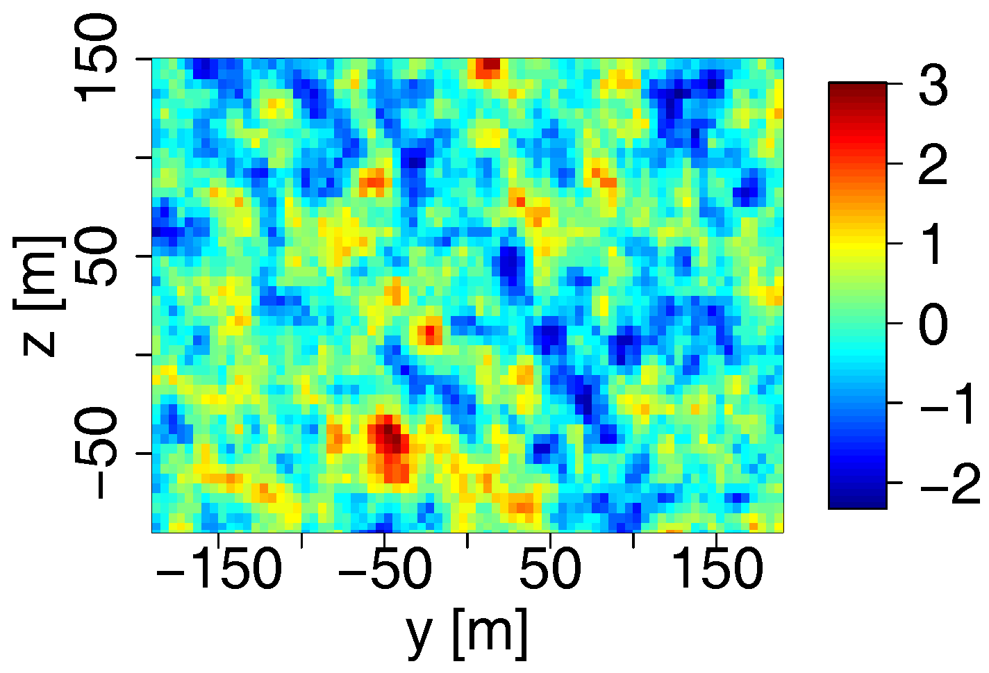
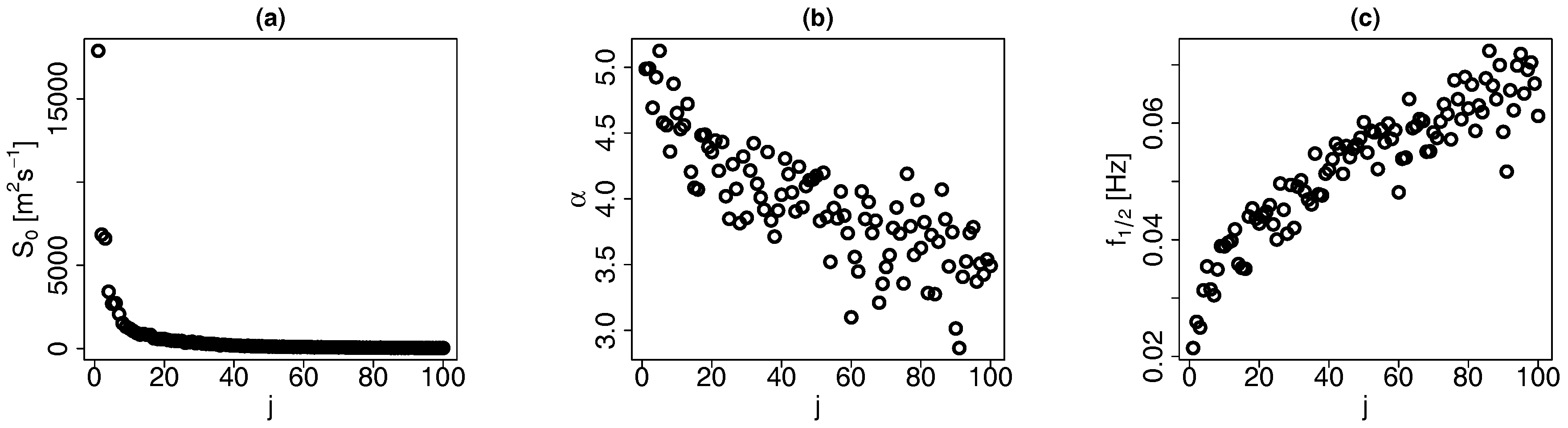
4.1. POD Modes and Eigenvalues
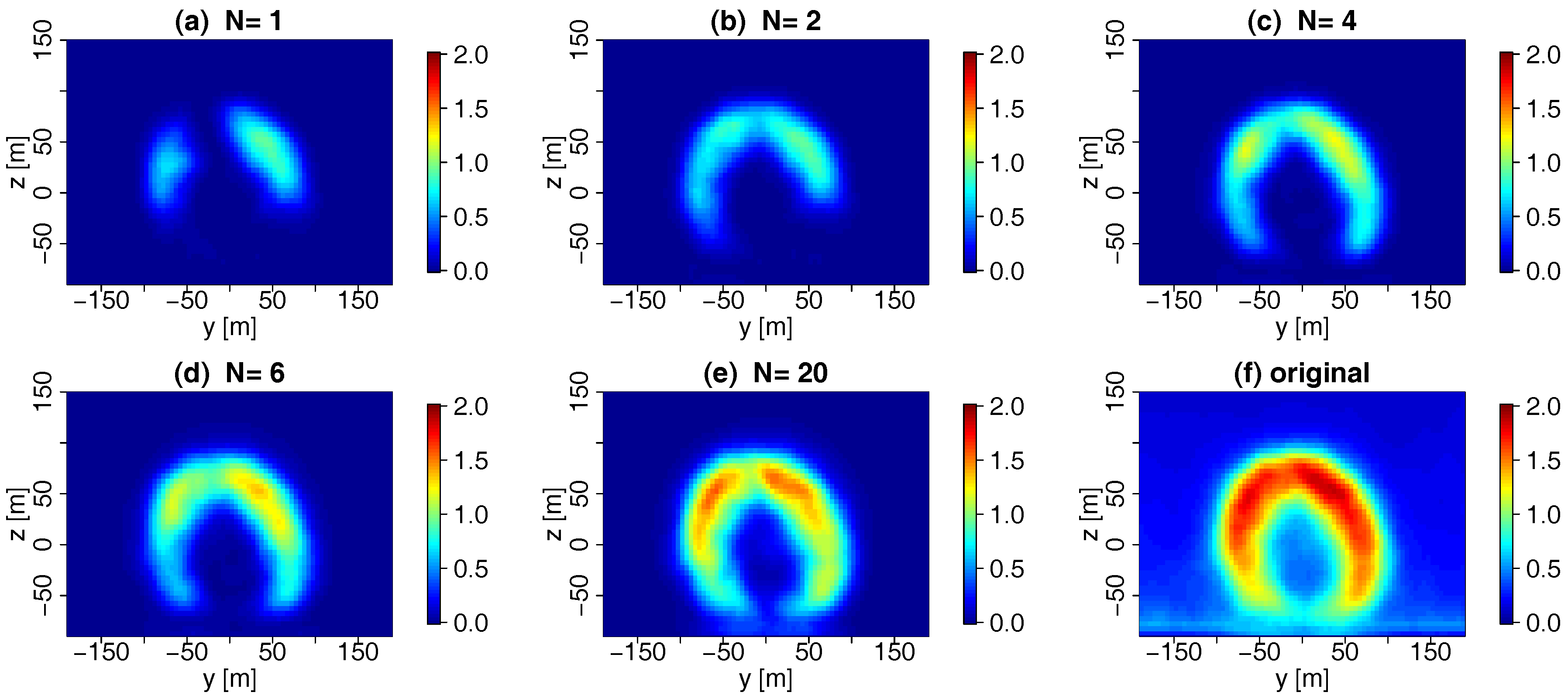
4.2. Performance of the Truncated PODs
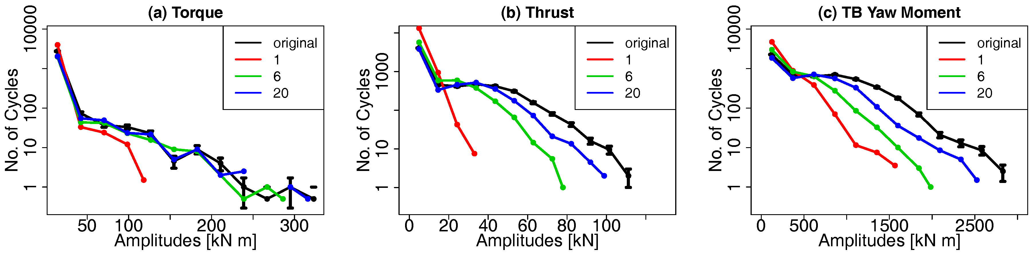
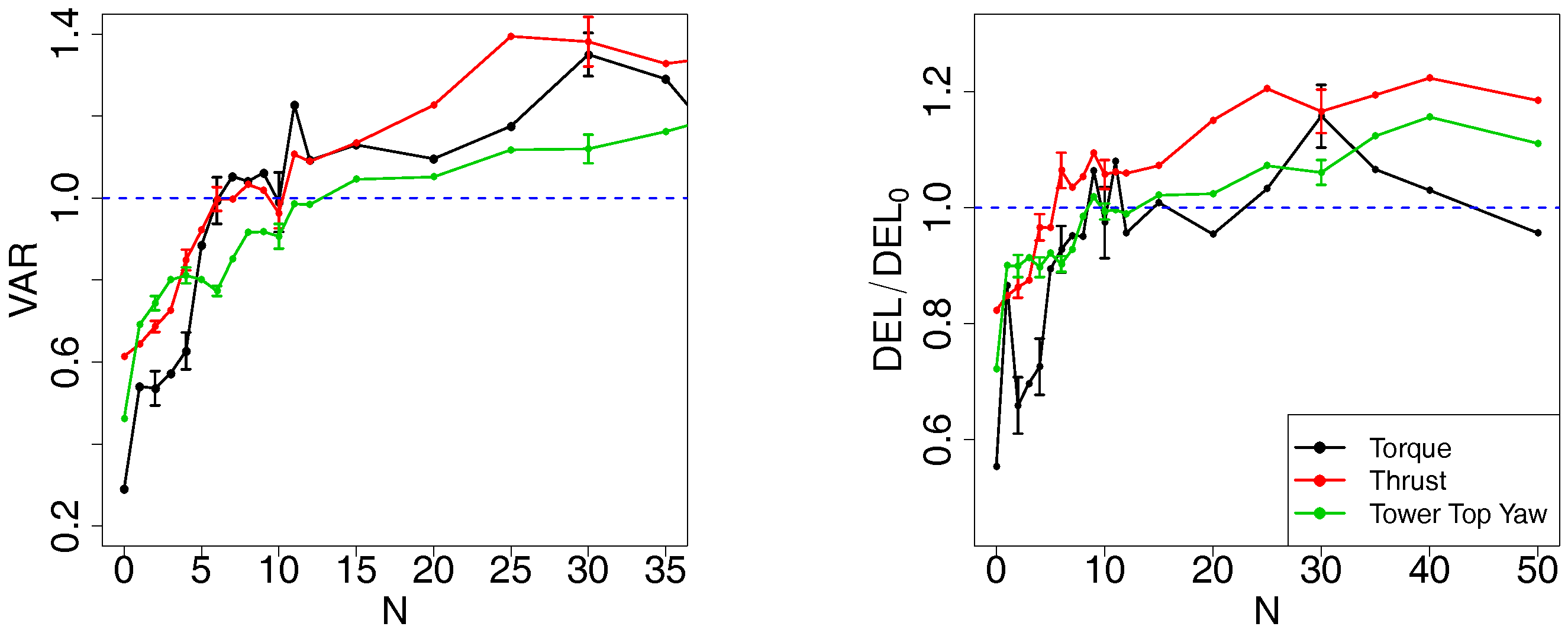
4.2.1. Results
4.2.2. Discussion
5. Stochastic Wake Models
5.1. Modeling the Weighting Coefficients
5.2. Performance of the Stochastic Wake Models
5.2.1. Results
5.2.2. Discussion
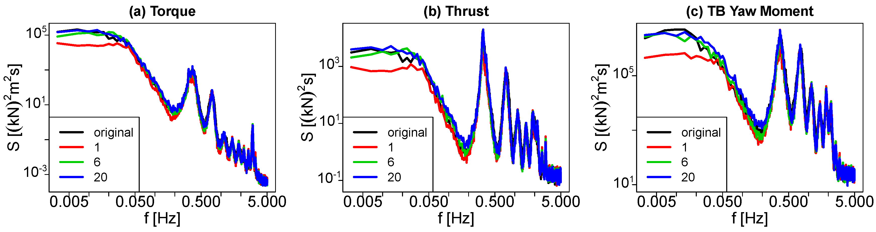
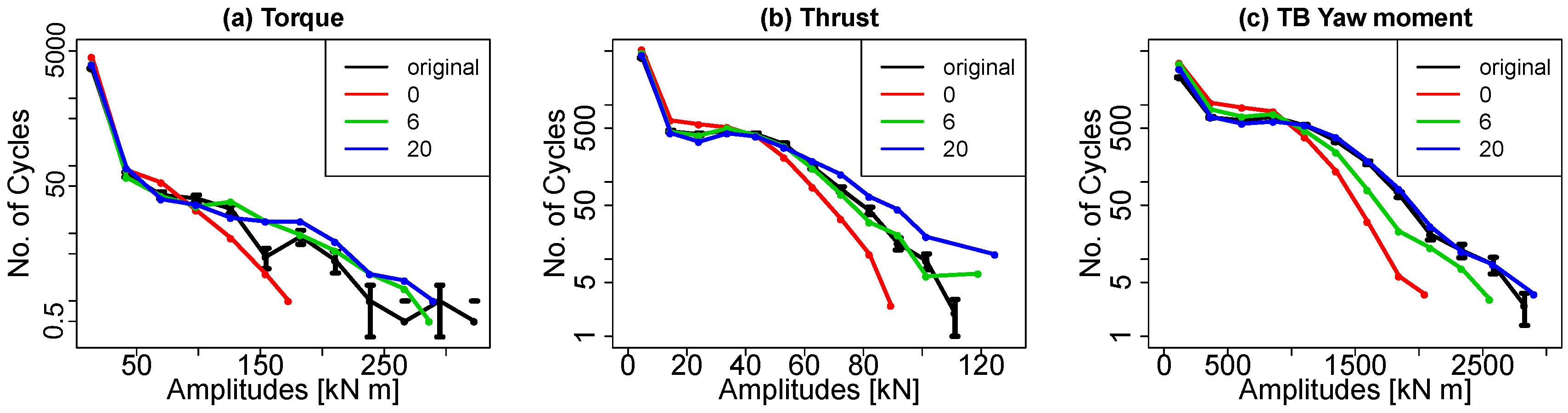
6. A Stochastic Wake Model with Added Turbulence
6.1. Basic Idea
6.2. Performance
6.2.1. Results
6.2.2. Discussion
7. Conclusions
Acknowledgments
Author Contributions
Conflicts of Interest
Appendix A. Details of the Spectral Model
Appendix A.1. Fitting Procedure
Appendix A.2. Estimated Parameters

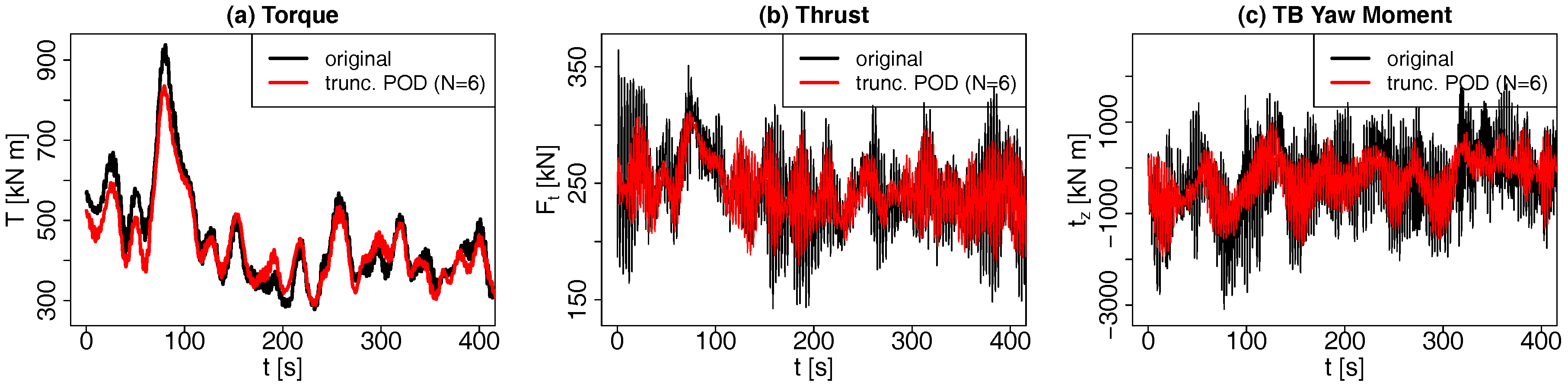
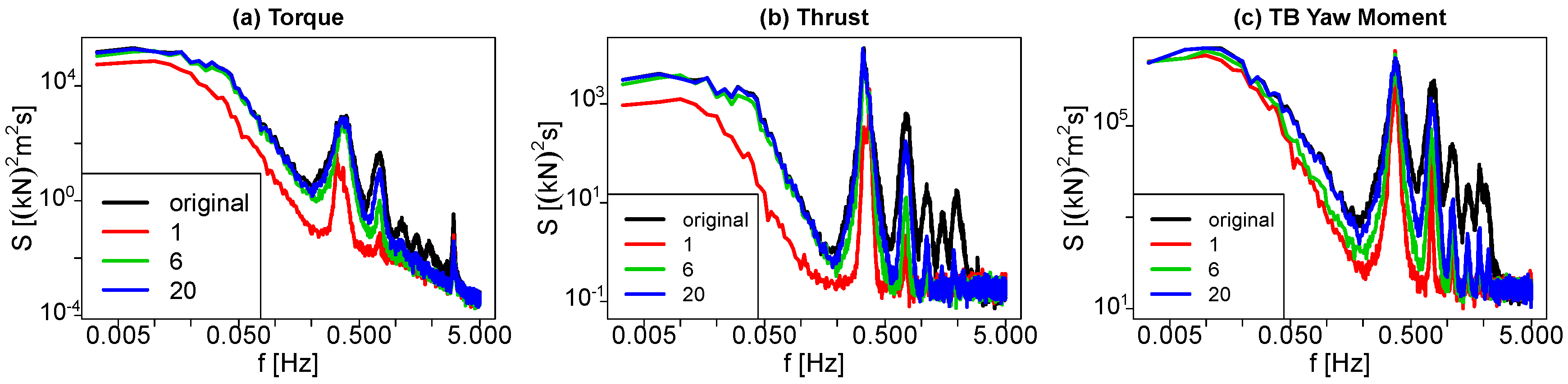
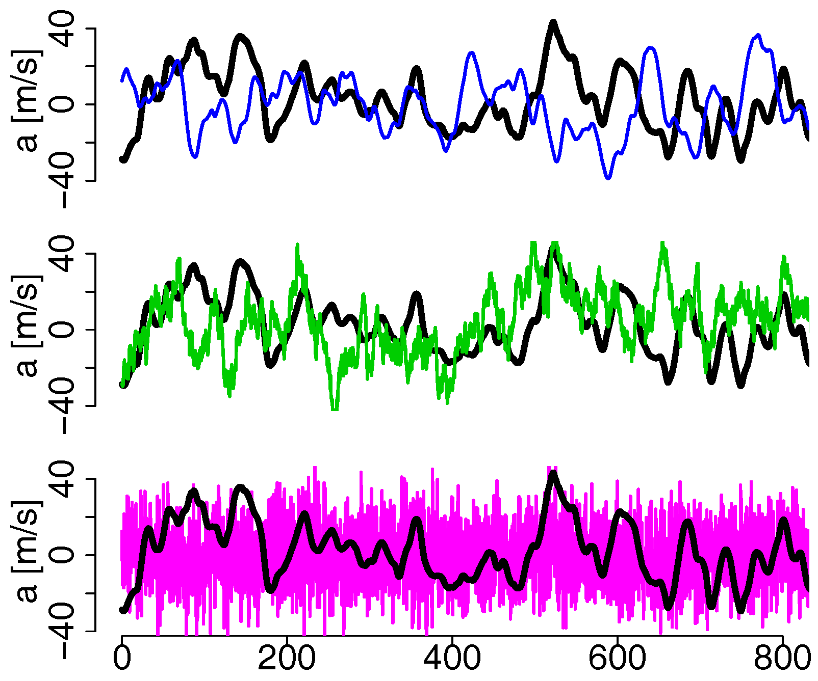
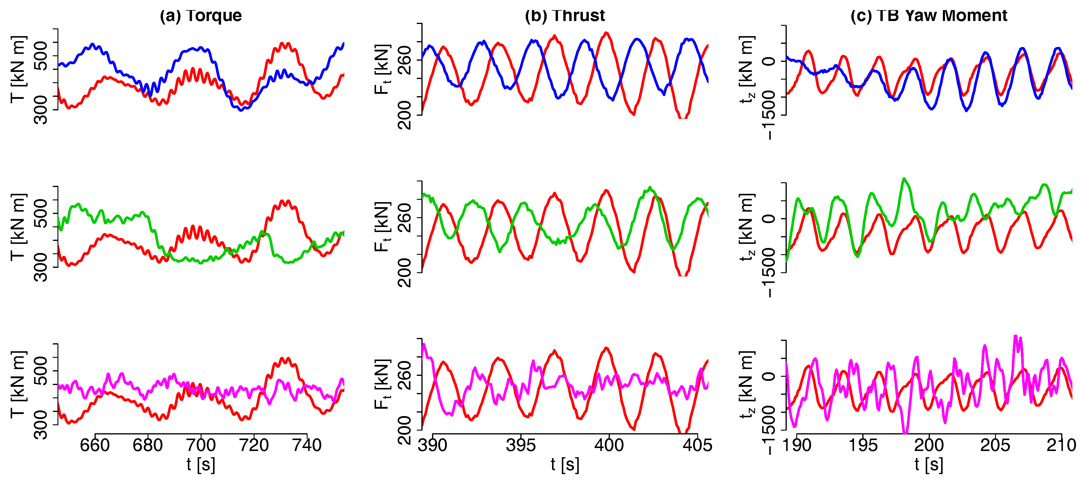
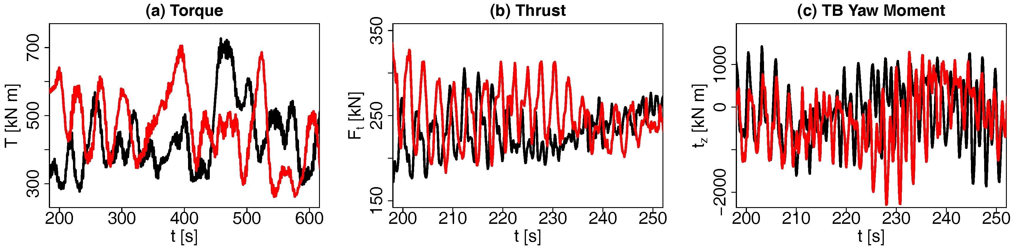
Appendix B. Time Series of Loads


References
- Barthelmie, R.J.; Frandsen, S.T.; Nielsen, M.; Pryor, S.; Rethore, P.E.; Jørgensen, H.E. Modelling and measurements of power losses and turbulence intensity in wind turbine wakes at Middelgrunden offshore wind farm. Wind Energy 2007, 10, 517–528. [Google Scholar] [CrossRef]
- Barthelmie, R.J.; Pryor, S.C.; Frandsen, S.T.; Hansen, K.S.; Schepers, J.G.; Rados, K.; Schlez, W.; Neubert, A.; Jensen, L.E.; Neckelmann, S. Quantifying the Impact of Wind Turbine Wakes on Power Output at Offshore Wind Farms. J. Atmos. Ocean. Technol. 2010, 27, 1302–1317. [Google Scholar] [CrossRef]
- Frandsen, S. Turbulence and Turbulence Generated Fatigue in Wind Turbine Clusters; Risø-R 1188; Risø National Laboratory: Roskilde, Denmark, 2005. [Google Scholar]
- Barthelmie, R.J.; Hansen, K.; Frandsen, S.T.; Rathmann, O.; Schepers, J.G.; Schlez, W.; Phillips, J.; Rados, K.; Zervos, A.; Politis, E.S.; et al. Modelling and Measuring Flow and Wind Turbine Wakes in Large Wind Farms Offshore. Wind Energy 2009, 12, 431–444. [Google Scholar] [CrossRef]
- Chowdhury, S.; Zhang, J.; Messac, A.; Castillo, L. Unrestricted wind farm layout optimization (UWFLO): Investigating key factors influencing the maximum power generation. Renew. Energy 2012, 38, 16–30. [Google Scholar] [CrossRef]
- Gonzalez, J.S.; Payan, M.B.; Santos, J.M.R.; Gonzalez-Longatt, F. A review and recent developments in the optimal wind-turbine micro-siting problem. Renew. Sustain. Energy Rev. 2014, 30, 133–144. [Google Scholar] [CrossRef]
- Schmidt, J.; Stoevesandt, B. Wind Farm Layout Optimisation Using Wakes from Computational Fluid Dynamics Simulations. In Proceedings of the EWEA Conference, Barcelona, Spain, 10–13 March 2014. [Google Scholar]
- Corten, G.; Schaak, P. Heat and flux: increase of wind farm production by reduction of the axial induction. In Proceedings of the European Wind Energy Conference, Madrid, Spain, 16–19 June 2003. [Google Scholar]
- Fleming, P.A.; Gebraad, P.M.O.; Lee, S.; van Wingerden, J.W.; Johnson, K.; Churchfield, M.; Michalakes, J.; Spalart, P.; Moriarty, P. Evaluating techniques for redirecting turbine wakes using SOWFA. Renew. Energy 2014, 70, 211–218. [Google Scholar] [CrossRef]
- Annoni, J.; Gebraad, P.M.O.; Scholbrock, A.K.; Fleming, P.A.; van Wingerden, J.W. Analysis of axial-induction-based wind plant control using an engineering and a high-order wind plant model. Wind Energy 2016, 19, 1135–1150. [Google Scholar] [CrossRef]
- Gebraad, P.M.O.; Teeuwisse, F.W.; van Wingerden, J.W.; Fleming, P.A.; Ruben, S.D.; Marden, J.R.; Pao, L.Y. Wind plant power optimization through yaw control using a parametric model for wake effects-a CFD simulation study. Wind Energy 2016, 19, 95–114. [Google Scholar] [CrossRef]
- Ferrer, E.; Browne, O.M.; Valero, E. Sensitivity Analysis to Control the Far-Wake Unsteadiness Behind Turbines. Energies 2017, 10, 1599. [Google Scholar] [CrossRef]
- Frisch, U. Turbulence; Cambridge University Press: Cambridge, UK, 1995. [Google Scholar]
- Pope, S.B. Turbulent Flows; Cambridge University Press: Cambridge, UK, 2000. [Google Scholar]
- Mikkelsen, R. Actuator Disc Methods Applied to Wind Turbines. Ph.D. Thesis, Technical University of Denmark, Lyngby, Denmark, 2003. [Google Scholar]
- Calaf, M.; Meneveau, C.; Meyers, J. Large eddy simulation study of fully developed wind-turbine array boundary layers. Phys. Fluids 2010, 22, 015110. [Google Scholar] [CrossRef]
- Lu, H.; Porte-Agel, F. Large-eddy simulation of a very large wind farm in a stable atmospheric boundary layer. Phys. Fluids 2011, 23, 065101. [Google Scholar] [CrossRef]
- Wu, Y.T.; Porte-Agel, F. Large-Eddy Simulation of Wind-Turbine Wakes: Evaluation of Turbine Parametrisations. Bound.-Layer Meteorol. 2011, 138, 345–366. [Google Scholar]
- Porté-Agel, F.; Wu, Y.T.; Lu, H.; Conzemius, R.J. Large-eddy simulation of atmospheric boundary layer flow through wind turbines and wind farms. J. Wind Eng. Ind. Aerodyn. 2011, 99, 154–168. [Google Scholar] [CrossRef]
- Goit, J.P.; Meyers, J. Analysis of turbulent flow properties and energy fluxes in optimally controlled wind-farm boundary layers. J. Phys. Conf. Ser. 2014, 524, 012178. [Google Scholar] [CrossRef]
- VerHulst, C.; Meneveau, C. Large eddy simulation study of the kinetic energy entrainment by energetic turbulent flow structures in large wind farms. Phys. Fluids 2014, 26, 025113. [Google Scholar] [CrossRef]
- Witha, B.; Steinfeld, G.; Heinemann, D. High-resolution offshore wake simulations with the LES model PALM. In Wind Energy-Impact Turbul; Springer: Berlin/Heidelberg, Germany, 2014. [Google Scholar]
- Dörenkämper, M.; Witha, B.; Steinfeld, G.; Heinemann, D.; Kühn, M. The impact of stable atmospheric boundary layers on wind-turbine wakes within offshore wind farms. J. Wind Eng. Ind. Aerodyn. 2015, 144, 146–153. [Google Scholar] [CrossRef]
- Stevens, R.J.A.M.; Gayme, D.F.; Meneveau, C. Effects of turbine spacing on the power output of extended wind-farms. Wind Energy 2016, 19, 359–370. [Google Scholar] [CrossRef]
- Jensen, N.O. A Note on Wind Generator Interaction; Risø National Laboratory: Roskilde, Denmark, 1983. [Google Scholar]
- Frandsen, S.; Barthelmie, R.; Pryor, S.; Rathmann, O.; Larsen, S.; Hojstrup, J.; Thogersen, M. Analytical modelling of wind speed deficit in large offshore wind farms. Wind Energy 2006, 9, 39–53. [Google Scholar] [CrossRef]
- Quarton, D.; Ainslie, J. Turbulence in wind turbine wakes. Wind Eng. 1990, 14, 15–23. [Google Scholar]
- Larsen, G.C.; Madsen Aagaard, H.; Bingöl, F.; Mann, J.; Ott, S.; Sørensen, J.N.; Okulov, V.; Troldborg, N.; Nielsen, N.M.; Thomsen, K. Dynamic Wake Meandering Modeling; Risø-R 1607; Risø National Laboratory: Roskilde, Denmark, 2007. [Google Scholar]
- Larsen, G.C.; Madsen, H.A.; Thomsen, K.; Larsen, T.J. Wake meandering: A pragmatic approach. Wind Energy 2008, 11, 377–395. [Google Scholar] [CrossRef]
- Madsen, H.A.; Larsen, G.C.; Larsen, T.J.; Troldborg, N.; Mikkelsen, R. Calibration and validation of the dynamic wake meandering model for implementation in an aeroelastic code. J. Sol. Energy Eng. 2010, 132, 041014. [Google Scholar] [CrossRef]
- Keck, R.E.; Maré, M.; Churchfield, M.J.; Lee, S.; Larsen, G.; Madsen, H.A. Two improvements to the dynamic wake meandering model: including the effects of atmospheric shear on wake turbulence and incorporating turbulence build-up in a row of wind turbines. Wind Energy 2015, 18, 111–132. [Google Scholar] [CrossRef]
- Larsen, T.J.; Madsen, H.A.; Larsen, G.C.; Hansen, K.S. Validation of the dynamic wake meander model for loads and power production in the Egmond aan Zee wind farm. Wind Energy 2013, 16, 605–624. [Google Scholar] [CrossRef]
- Singh, A.; Howard, K.B.; Guala, M. On the homogenization of turbulent flow structures in the wake of a model wind turbine. Phys. Fluids 2014, 26. [Google Scholar] [CrossRef]
- Bastine, D.; Wächter, M.; Peinke, J.; Trabucchi, D.; Kühn, M. Characterizing Wake Turbulence with Staring Lidar Measurements. J. Phys. Conf. Ser. 2015, 625, 012006. [Google Scholar] [CrossRef]
- Andersen, S.J.; Sørensen, J.N.; Mikkelsen, R. Reduced order model of the inherent turbulence of wind turbine wakes inside an infinitely long row of turbines. J. Phys. Conf. Ser. 2014, 555, 012005. [Google Scholar] [CrossRef]
- Andersen, S.J.; Sorensen, J.N.; Mikkelsen, R. Simulation of the inherent turbulence and wake interaction inside an infinitely long row of wind turbines. J. Turbul. 2013, 14, 1–24. [Google Scholar] [CrossRef]
- Bastine, D.; Witha, B.; Wächter, M.; Peinke, J. POD Analysis of a Wind Turbine Wake in a Turbulent Atmospheric Boundary Layer. J. Phys. Conf. Ser. 2014, 524, 012153. [Google Scholar] [CrossRef]
- Bastine, D.; Witha, B.; Wächter, M.; Peinke, J. Towards a Simplified DynamicWake Model Using POD Analysis. Energies 2015, 8, 895–920. [Google Scholar] [CrossRef]
- Hamilton, N.; Tutkun, M.; Cal, R.B. Wind turbine boundary layer arrays for Cartesian and staggered configurations: Part II, low-dimensional representations via the proper orthogonal decomposition. Wind Energy 2015, 18, 297–315. [Google Scholar] [CrossRef]
- Hamilton, N.; Tutkun, M.; Cal, R.B. Low-order representations of the canonical wind turbine array boundary layer via double proper orthogonal decomposition. Phys. Fluids 2016, 28, 025103. [Google Scholar] [CrossRef]
- Iungo, G.V.; Santoni-Ortiz, C.; Abkar, M.; Porté-Agel, F.; Rotea, M.A.; Leonardi, S. Data-driven Reduced Order Model for prediction of wind turbine wakes. J. Phys. Conf. Ser. 2015, 625, 012009. [Google Scholar] [CrossRef]
- Sarmast, S.; Dadfar, R.; Mikkelsen, R.F.; Schlatter, P.; Ivanell, S.; Sorensen, J.N.; Henningson, D.S. Mutual inductance instability of the tip vortices behind a wind turbine. J. Fluid Mech. 2014, 755, 705–731. [Google Scholar] [CrossRef]
- Debnath, M.; Santoni, C.; Leonardi, S.; Iungo, G.V. Towards reduced order modelling for predicting the dynamics of coherent vorticity structures within wind turbine wakes. Philos. Trans. A Math. Phys. Eng. Sci. 2017, 375. [Google Scholar] [CrossRef] [PubMed]
- Ali, N.; Cortina, G.; Hamilton, N.; Calaf, M.; Cal, R.B. Turbulence characteristics of a thermally stratified wind turbine array boundary layer via proper orthogonal decomposition. J. Fluid Mech. 2017, 828, 175–195. [Google Scholar] [CrossRef]
- Araya, D.B.; Colonius, T.; Dabiri, J.O. Transition to bluff-body dynamics in the wake of vertical-axis wind turbines. J. Fluid Mech. 2017, 813, 346–381. [Google Scholar] [CrossRef]
- Tabib, M.; Siddiqui, M.S.; Fonn, E.; Rasheed, A.; Kvamsdal, T. Near wake region of an industrial scale wind turbine: comparing LES-ALM with LES-SMI simulations using data mining (POD). J. Phys. Conf. Ser. 2017, 854, 012044. [Google Scholar] [CrossRef]
- Hamilton, N.; Tutkun, M.; Cal, R.B. Anisotropic character of low-order turbulent flow descriptions through the proper orthogonal decomposition. Phys. Rev. Fluids 2017, 2. [Google Scholar] [CrossRef]
- Berkooz, G.; Holmes, P.; Lumley, J.L. The Proper Orthogonal Decomposition In the Analysis of Turbulent Flows. Ann. Rev. Fluid Mech. 1993, 25, 539–575. [Google Scholar] [CrossRef]
- Cordier, L.; Noack, B.R.; Tissot, G.; Lehnasch, G.; Delville, J.; Balajewicz, M.; Daviller, G.; Niven, R.K. Identification strategies for model-based control. Exp. Fluids 2013, 54, 1580. [Google Scholar] [CrossRef]
- Schmid, P.J. Dynamic mode decomposition of numerical and experimental data. J. Fluid Mech. 2010, 656, 5–28. [Google Scholar] [CrossRef]
- Jovanović, M.R.; Schmid, P.J.; Nichols, J.W. Sparsity-promoting dynamic mode decomposition. Phys. Fluids 2014, 26, 024103. [Google Scholar] [CrossRef]
- Le Clainche, S.; Vega, J.M. Higher order dynamic mode decomposition to identify and extrapolate flow patterns. Phys. Fluids 2017, 29, 084102. [Google Scholar] [CrossRef]
- Kou, J.; Le Clainche, S.; Zhang, W. A reduced-order model for compressible flows with buffeting condition using higher order dynamic mode decomposition with a mode selection criterion. Phys. Fluids 2018, 30, 016103. [Google Scholar] [CrossRef]
- Andersen, S.J. Simulation and Prediction of Wakes and Wake Interaction in Wind Farms. Ph.D. Thesis, Technical University of Denmark, Lyngby, Denmark, 2014. [Google Scholar]
- Iungo, G.V.; Wu, Y.T.; Porte-Agel, F. Field Measurements of Wind Turbine Wakes with Lidars. J. Atmos. Ocean. Technol. 2013, 30, 274–287. [Google Scholar] [CrossRef]
- Witha, B.; Steinfeld, G.; Heinemann, D. Advanced turbine parameterizations in offshore LES wake simulations. In Proceedings of the 6th Intenational Symposium on Computational Wind Engineering, Hamburg, Germany, 8–13 June 2014. [Google Scholar]
- Raasch, S.; Schroter, M. PALM—A large-eddy simulation model performing on massively parallel computers. Meteorol. Z. 2001, 10, 363–372. [Google Scholar] [CrossRef]
- Maronga, B.; Gryschka, M.; Heinze, R.; Hoffmann, F.; Kanani-Sühring, F.; Keck, M.; Ketelsen, K.; Letzel, M.O.; Sühring, M.; Raasch, S. The Parallelized Large-Eddy Simulation Model (PALM) version 4.0 for atmospheric and oceanic flows: Model formulation, recent developments, and future perspectives. Geosci. Model Dev. 2015, 8, 2515–2551. [Google Scholar] [CrossRef]
- Deardorff, J.W. Stratocumulus-capped mixed layers derived from a three-dimensional model. Bound.-Layer Meteorol. 1980, 18, 495–527. [Google Scholar] [CrossRef]
- Vollmer, L.; Steinfeld, G.; Heinemann, D.; Kühn, M. Estimating the wake deflection downstream of a wind turbine in different atmospheric stabilities: An LES study. Wind Energy Sci. Discuss. 2016, 1, 129–141. [Google Scholar] [CrossRef]
- Wang, T. A brief review on wind turbine aerodynamics. Theor. Appl. Mech. Lett. 2012, 2, 062001. [Google Scholar] [CrossRef]
- Jonkman, J.M.; Butterfield, S.; Musial, W.; Scott, G. Definition of a 5-MW Reference Wind Turbine for Offshore System Development; Technical Report NREL/TP-500-38060; National Renewable Energy Laboratory: Golden, CO, USA, 2009.
- Serra, J. Image Analysis and Mathematical Morphology, V. 1; Academic Press: New York, NY, USA, 1982. [Google Scholar]
- Risken, H. Fokker-Planck Equation; Springer: New York, NY, USA, 1984. [Google Scholar]
- Gardiner, C.W. Handbook of Stochastic Methods; Springer: Berlin, Germany, 1985; Volume 3. [Google Scholar]
- Friedrich, R.; Peinke, J.; Sahimi, M.; Reza Rahimi Tabar, M. Approaching complexity by stochastic methods: From biological systems to turbulence. Phys. Rep. 2011, 506, 87–162. [Google Scholar] [CrossRef]
- Kantz, H.; Schreiber, T. Nonlinear Time Series Analysis; Cambridge University Press: Cambridge, UK, 2004; Volume 7. [Google Scholar]
- Jonkman, J.M.; Buhl, M.L., Jr. FAST User’s Guide, NREL/EL-500-29798; Technical Report; National Renewable Energy Laboratory: Golden, Colorado, USA, 2005.
- Laino, D. NWTC Design Code AeroDyn v12.58; Technical Report; National Renewable Energy Laboratory: Golden, CO, USA, 2005.
- Burton, T.; Sharpe, D.; Jenkins, N.; Bossanyi, E. Wind Energy Handbook; Wiley: New York, NY, USA, 2011. [Google Scholar]
- Nieslony, A. Rainflow Counting Algorithm (Version 1.2); Mathworks, Matlab Central: Natick, CA, USA, 2010. [Google Scholar]
- ASTM E1049-85. Standard Practices for Cycle Counting in Fatigue Analysis; ASTM: West Conshohocken, PA, USA, 1994. [Google Scholar]
- Saranyasoontorn, K.; Manuel, L. Low-dimensional representations of inflow turbulence and wind turbine response using proper orthogonal decomposition. J. Sol. Energy Eng. 2005, 127, 553–562. [Google Scholar] [CrossRef]
- Saranyasoontorn, K.; Manuel, L. Symmetry considerations when using proper orthogonal decomposition for predicting wind turbine yaw loads. J. Sol. Energy Eng.-Trans. 2006, 128, 574–579. [Google Scholar] [CrossRef]
- Mann, J. Wind field simulation. Probab. Eng. Mech. 1998, 13, 269–282. [Google Scholar] [CrossRef]
- Kleinhans, D. Stochastische Modellierung Komplexer Systeme—Von den Theoretischen Grundlagen zur Simulation Atmosphärischer Windfelder. Ph.D. Thesis, University of Münster, Münster, Germany, 2008. [Google Scholar]
- Beck, H.; Davide, T.; Andreas, R.; vanDooren, M.; Kühn, M. Volumetric wind field measurements of wind turbine wakes with long-range lidars. In Proceedings of the EWEA Conference, Paris, France, 17–20 November 2015. [Google Scholar]
- Barthelmie, R.J.; Doubrawa, P.; Wang, H.; Pryor, S.C. Defining wake characteristics from scanning and vertical full-scale lidar measurements. J. Phys. Conf. Ser. 2016, 753, 032034. [Google Scholar] [CrossRef]
- Chamorro, L.P.; Guala, M.; Arndt, R.E.A.; Sotiropoulos, F. On the evolution of turbulent scales in the wake of a wind turbine model. J. Turbul. 2012, 13. [Google Scholar] [CrossRef]
- Melius, M.S.; Tutkun, M.; Cal, R.B. Identification of Markov process within a wind turbine array boundary layer. J. Renew. Sustain. Energy 2014, 6, 023121. [Google Scholar] [CrossRef]
- Melius, M.S.; Tutkun, M.; Cal, R.B. Solution of the Fokker–Planck equation in a wind turbine array boundary layer. Phys. D Nonlinear Phenom. 2014, 280, 14–21. [Google Scholar] [CrossRef]


© 2018 by the authors. Licensee MDPI, Basel, Switzerland. This article is an open access article distributed under the terms and conditions of the Creative Commons Attribution (CC BY) license (http://creativecommons.org/licenses/by/4.0/).
Share and Cite
Bastine, D.; Vollmer, L.; Wächter, M.; Peinke, J. Stochastic Wake Modelling Based on POD Analysis. Energies 2018, 11, 612. https://doi.org/10.3390/en11030612
Bastine D, Vollmer L, Wächter M, Peinke J. Stochastic Wake Modelling Based on POD Analysis. Energies. 2018; 11(3):612. https://doi.org/10.3390/en11030612
Chicago/Turabian StyleBastine, David, Lukas Vollmer, Matthias Wächter, and Joachim Peinke. 2018. "Stochastic Wake Modelling Based on POD Analysis" Energies 11, no. 3: 612. https://doi.org/10.3390/en11030612
APA StyleBastine, D., Vollmer, L., Wächter, M., & Peinke, J. (2018). Stochastic Wake Modelling Based on POD Analysis. Energies, 11(3), 612. https://doi.org/10.3390/en11030612