Stationary Threshold Vector Autoregressive Models

Abstract

This paper examines the steady state properties of the Threshold Vector Autoregressive model. Assuming that the trigger variable is exogenous and the regime process follows a Bernoulli distribution, necessary and sufficient conditions for the existence of stationary distribution are derived. A situation related to so-called “locally explosive models”, where the stationary distribution exists though the model is explosive in one regime, is analysed. Simulations show that locally explosive models can generate some of the key properties of financial and economic data. They also show that assessing the stationarity of threshold models based on simulations might well lead to wrong conclusions.

1. Introduction

Correct theoretical and empirical modelling of financial time series remains challenging. First of all, the usual linear framework often falls short of properly describing the data, which, instead, exhibit important nonlinear features. Secondly, economic theory regularly results in models with multiple equilibria and asymmetries which the time series model should be able to accommodate. Finally, data is often interconnected and hence simple univariate models generally fall short of appropriately describing the complex nature of the data. The Global Financial Crisis in 2007–2008 demonstrated this very clearly and reinforced the need to use a multivariate nonlinear framework in economic models, in general, and in empirical finance, in particular.

Among the many possible candidate nonlinear models, threshold models are particularly interesting and they have been extensively used in the existing empirical literature. These models are straightforward generalizations of linear models. For example, the simple two regime Threshold Autoregressive (TAR) model specifies a different autoregressive structure for each of the regimes and a threshold variable that determines which regime is active. These models are therefore relatively simple to estimate, and, since at time t the regime state is known, they are more suitable for forecasting than other nonlinear models, in particular hidden Markov models. Finally, TAR models allow for reasonably simple tests of the linear structure against nonlinear alternatives and to test the number of regimes. The multivariate generalization of the TAR model instead uses vector autoregressive structures in the regimes and is therefore naturally referred to as the Threshold Vector AutoRegressive (TVAR) model (Hubrich and Teräsvirta 2013; Tsay 1998).

Empirical studies have used threshold models to explore the asymmetry of shocks and nonlinear relationship between variables in financial markets and data from the real and monetary economy. For instance, TVAR models are widely used to study the asymmetric effect of fiscal and monetary policies in different credit, interest rate and inflationary regimes (Balke 2000; Fazzari et al. 2015; Shen and Chiang 1999). Balke (2000), for example, studies the propagation of shocks to output growth, the Federal Funds rate, inflation and measures of credit conditions during “tight” and “normal” credit market conditions using a TVAR framework with two regimes. The results suggest that shocks have a larger effect on output in “tight” credit regimes and that contractionary monetary shocks are more effective than expansionary ones. A similar approach is followed by Calza and Souza (2006) to study the transmission of monetary shocks across two credit regimes in the EU area and by Li and St-Amant (2010) to evaluate the effect of financial stress conditions on monetary policy effectiveness in Canada.

Another important application of threshold models has been to study the business cycle. For example, Altissimo and Violante (2001) study the joint dynamics of US output and unemployment using a bivariate TVAR model for recessions and expansions. Here, the lagged feedback variable, which measures the depth of the recession, defines the regime. The resulting model is a VAR with a fixed number of lags when the economy is in expansion and a time varying lag order when the economy is in recession. The authors find that nonlinearities are statistically significant only for unemployment, but it transmits to output through cross-correlation. Further evidence on the usefulness of threshold models for analysing the business cycle can be found in Koop and Potter (1999), Peel and Speight (1998), Koop et al. (1996), and Potter (1995), amongst others.

Threshold models are also popular in financial markets studies to explore the asymmetric relation between variables. In particular, a common application of TAR models includes determining the threshold effect in price movements related to transaction cost (Yadav et al. 1994). The threshold autoregressive conditional heteroskedastic class of models has been applied to study the nonlinear effect in volatility processes (Rabemananjara and Zakoian 1993). Finally, multivariate threshold models have been extensively used in studying the dynamics in stock prices, returns, volatilities, inflation and economic activity (Barnes 1999; Griffin et al. 2007; Huang et al. 2005; Li et al. 2015). Griffin et al. (2007), for example, study the joint dynamics of stock market turnover, returns and volatility in 46 countries using a TVAR model with two regimes that are separated by the sign of the past return. The authors conclude that small negative return shocks, rather than large ones, are the drivers for the decrease in turnover after a decrease in returns. Li et al. (2015) study the interaction between Shanghai and Shenzhen stock markets in a bivariate three regime TVAR model where the threshold variable is the average difference of the log returns between the two markets. Their results suggest that the strength of interaction between markets is regime dependent. In particular, the Shanghai market leads most of the time, except for the third regime, where both markets interact simultaneously. A detailed review of the application of threshold models in empirical economics can be found in Hansen (2011).

One challenge with nonlinear time series models, in general, and by extension therefore also with threshold models, in particular, is to assess model stationarity. Establishing stationarity is important as it is a fundamental assumption in most theoretical research. Indeed, the asymptotic properties of estimators in threshold models are generally established under a set of standard regularity conditions, which include the existence of finite higher order moments and the strict stationarity of the data generating process (Tsay 1998). Moreover, existing inference approaches assume stationarity of the data generating process (Hansen 1996, 2000; Tsay 1998) and violation of this assumption might lead to spurious nonlinearity (Calza and Souza 2006) and could invalidate the use of, e.g., Hansen (1996) simulated p-values for inference.

While significant progress has been made to establish conditions which ensure stationarity for the univariate threshold case under realistic assumptions (Brockwell et al. 1992; Chan and Tong 1985; Chen et al. 2011; Knight and Satchell 2011; Petruccelli and Woolford 1984), to the best of our knowledge, very little is known about the multivariate extension. See Chen et al. (2011) for an extensive review about recent findings regarding the stationarity of TAR models. If one was to use the general approach from this literature to establish the stationarity of TVAR models, it would require proving the convergence of an infinite sum of products of random matrices. This is clearly difficult and likely explains the absence of theoretical results for the TVAR model.

In this paper, we fill this gap in the existing literature and analyse the properties of the TVAR model in detail. To achieve this, we assume that the trigger variable is exogenous and that the regime process follows a Bernoulli distribution. We first derive necessary and sufficient conditions for second order stationarity, which are not present in the previous literature, when the variance–covariance matrices of the random vector and the error process are assumed to have full rank. Next, we characterize the joint conditional distribution of the data generating process when the error vector follows a multivariate normal distribution. Finally, we derive the unconditional distribution for a special case of the TVAR model, and we demonstrate that, in this case, the distribution of the threshold model is an infinite mixture of normals. This shows that TVAR models are very general and can accommodate many of the stylized features of financial data.

As a first interesting application of our results, we consider the special case where the elements of the random vector are positively correlated and we describe a model that is explosive in one regime, but still allows for the existence of steady state distribution. A similar idea was introduced in Knight et al. (2014) in the univariate case as a so-called “locally explosive model”. In particular, they study the univariate threshold autoregressive model with exogenous trigger and its application to bubble formation. We expand the notion of locally explosive models to the bivariate TVAR model. The derived conditions for the existence of the stationary distribution have simple economic intuition and are easy to interpret. In particular, our results show that, in the stationary model, there is a trade-off between autoregressive dependence in the regime and the probability of the regime.

Next, we conduct an empirical analysis of the locally explosive models. In the absence of explicit theoretical conditions that guarantee stationarity of the model, the previous literature suggested to establish stationarity indirectly by demonstrating, using a simulation study, that the estimated model does not appear to contradict the stability assumption. To assess this procedure, we simulate the bivariate locally explosive TVAR model for different distributions of the regimes. Our results show that a simulation study aimed at verifying stability of a particular model might give inconclusive or even wrong results. Specifically, we show that the simulation exercise may very well fail to reject stability of non-stationary TVAR models when the probability of the explosive regime is low.

Finally, we empirically document that the locally explosive TVAR model can be associated with bubble formation processes. In fact, our simulated locally explosive models appear to possess explosive and unit root behaviour while overall remaining stationary. These properties are implied by the definition of bubbles prevailing in the current literature and formally described by Evans (1991) and Phillips and Yu (2011). Our results, therefore, should encourage further research into multivariate threshold models and their use to study the formation of and existence of bubbles in financial data.

The structure of the paper is as follows: In Section 2, we derive the necessary and sufficient conditions for second order stationarity and for the existence of a stationary distribution for the TVAR model. This section also derives closed form solutions for the stationary distribution. In Section 3, we consider the so-called locally explosive models, in which the TVAR model is explosive in one regime, while overall remaining stationary. This section also presents some interesting special cases and reports the results from a simulation study. Finally, Section 4 concludes the paper. All proofs can be found in Appendix A and Appendix B contains additional figures.

2. The Threshold Vector Autoregressive Model

Throughout this paper, we consider the threshold vector autoregressive model given by

$$Y_t={\Phi }^{1}I(X_{t-1}\in R_1)Y_{t-1}+{\Phi }^{2}I(X_{t-1}\in R_2)Y_{t-1}+{ϵ}_t,$$

(1)

where $Y_t$ is a $(n\times 1)$ random vector, ${\Phi }^1$ and ${\Phi }^2$ are $(n\times n)$ parameter matrices, where n is the number of time series, $I()$ is the indicator function, $X_t$ is an $iid$ random variable, which determines the regime, and ${ϵ}_t$ is a sequence of independent multivariate random vectors, such that $E({ϵ}_t)=0$ and $Var({ϵ}_t)=\Sigma$, $\forall t$, where $\Sigma$ is positive definite with full rank. We assume that $E({ϵ}_t|X_s)=0$ for all $s\le t$ and that the sequence $({ϵ}_t,X_t)$, $t\ge 1$, is $iid$.

The regime process is defined as $S_t=I(X_t\in R_2)$, $\forall t$, where $Prob(X_t\in R_2)=\pi$ and $Prob(X_t\in R_1)=1-\pi$, with $R_1\cup R_2=R$ and $R_1\cap R_2=\varnothing$. From this, it follows that $S_t$ is an $iid$ Bernoulli variable with $S_t=0$ with probability $1-\pi$ and $S_t=1$ with probability $\pi$. Using $S_t$, Equation (1) can be rewritten as $Y_t=({\Phi }^1+S_{t-1}{\Phi }^0)Y_{t-1}+{ϵ}_t$, where ${\Phi }^0={\Phi }^2-{\Phi }^1$. If we further denote by $B_t=S_t{\Phi }^0-\pi {\Phi }^0$, where $E(B_t)=0$, $\forall t$, the model in Equation (1) can be rewritten as a Random Coefficient Model (RCM) (see Nicholls and Quinn (1982)) given by

$$Y_t=(\Phi +B_{t-1})Y_{t-1}+{ϵ}_t,$$

(2)

where $\Phi ={\Phi }^1+\pi {\Phi }^0=(1-\pi ){\Phi }^1+\pi {\Phi }^2$.

In the following sections, we examine the TVAR model specified above in detail. First, we provide the necessary and sufficient conditions under which the TVAR model is second order stationary. We also derive expressions for the moments and the stationary solution to the model given in Equation (1). Secondly, we derive the distribution associated with this data generating process. For simplicity, we assume only two regimes in Equation (1). However, the theoretical results obtained here can easily be generalized to multiple regimes.

2.1. Stationarity of the TVAR Model

Theorem 1 provides conditions under which the TVAR model above is second order stationary, i.e., that $E(Y_t)$ is constant and $Cov(Y_t,Y_{t+h})$ depends only on the lag h.

Theorem 1.

The process $Y_t$, $t=0,1,2,\dots$ defined in Equation (1) is second order stationary with positive definite covariance matrix $V=Var(Y_0)$ if and only if:

1.

$\mu =0$, where μ is a mean of the initial vector, $\mu =E(Y_0)$,

2.

the covariance matrix V solves $V-\Phi V{\Phi }^{\prime }-E(B_{t-1}V{B}_{t-1}^{\prime })=\Sigma$, and

3.

$\mid \lambda \mid <1$, where λ is the maximum eigenvalue of the matrix $(1-\pi ){\Phi }^1\otimes {\Phi }^1+\pi {\Phi }^2\otimes {\Phi }^2$.

Proof. 

See Appendix A. ☐

Condition 3 of Theorem 1 provides a simple and intuitive eigenvalue condition for establishing second order stationarity of the TVAR model in Equation (1). We note that conditions similar to what we present here have been derived previously, though this has been done using alternative and, we believe, less realistic and empirically interesting assumptions (see, e.g., Nicholls and Quinn (1981), Feigin and Tweedie (1985) and Saikkonen (2007)). In particular, Nicholls and Quinn (1981), Feigin and Tweedie (1985) as well as Saikkonen (2007) assume independence of the error term, ${ϵ}_t$, and the threshold variable, $X_t$. We do not have this assumption and instead make a, we believe, far less restrictive assumption of the exogeneity of the threshold variable, $X_t$, i.e., $E({ϵ}_t|X_t)$, which does not rule out, for example, the possibility that the threshold variable $X_t$ could be a part of the ${ϵ}_t$ process.

Condition 2 of Theorem 1 provides an expression for calculating the covariance matrix of the second order stationary process $Y_t$. Notice that, after vectorization of this expression, we can obtain a closed form formula for this. Remark 1 provides this formula.

Remark 1.

From vectorization of the expression $V-\Phi V{\Phi }^{\prime }-E(B_{t-1}V{B}_{t-1}^{\prime })=\Sigma$, the equation for the variance of $Y_t$ can be obtained from

$$vecV={(I-\Phi \otimes \Phi -\pi (1-\pi ){\Phi }^0\otimes {\Phi }^0)}^{-1}vec\Sigma .$$

(3)

Theorem 2 provides an expression for the stationary solution to the model in Equation (1) and the corresponding conditions for the existence of this solution. Theorem 2 also shows that this solution is unique and strictly stationary.

Theorem 2.

Assume that V is positive definite with full rank. Then, the TVAR model in Equation (1) has a unique stationary solution given by

$$Y_t={ϵ}_t+\sum _{n=1}^{\infty }\left(\prod _{k=1}^n\Phi +B_{t-k}\right){ϵ}_{t-n},$$

(4)

if and only if $\mid \lambda \mid <1$, where λ is the maximum eigenvalue of the matrix $(1-\pi ){\Phi }^1\otimes {\Phi }^1+\pi {\Phi }^2\otimes {\Phi }^2$.

Proof. 

See Appendix A. ☐

In Remark 2, we provide the restriction on the eigenvalues of the matrix $\Phi$, which is necessary for the stationary model in Equation (1) and follows from Theorems 1 and 2. This condition is more tractable, and it is used in Section 3 to simplify the analysis of the stationary TVAR model with one explosive regime.

Remark 2.

Let the process $Y_t$, $t=0,1,2,\dots$ defined in Equation (1) be stationary with positive definite covariance matrix V. Then, the maximum eigenvalue of the matrix Φ is less than 1.

Proof. 

See Appendix A. ☐

The results of Theorems 1 and 2 can be extended to TVAR models with more than one lag. Corollary 1 presents the conditions for the stationarity of the TVAR model, which contains more than one lag.

Corollary 1.

Consider the following two-regime TVAR model with p lags in each regime

$$Y_t=I(X_{t-1}\in R_1)\sum _{j=1}^p{\Phi }^{1j}{Y}_{t-j}+I(X_{t-1}\in R_2)\sum _{j=1}^p{\Phi }^{2j}{Y}_{t-j}+{ϵ}_t,$$

(5)

where the properties of $X_t$ and ${ϵ}_t$ are those following Equation (1). This model has a unique stationary solution given by

$$Z_t={\eta }_t+\sum _{n=1}^{\infty }\left(\prod _{k=1}^{n}A+D_{t-k}\right){\eta }_{t-n},$$

(6)

where $Z_t$ and ${\eta }_t$ are $np\times 1$ vectors given by $Z_t^{\prime }=[Y_t^{\prime },Y_{t-1}^{\prime },Y_{t-2}^{\prime },\dots Y_{t-(p-1)}^{\prime }]$ and ${\eta }_t=[{ϵ}_t^{\prime },0,0,\dots ,0]$, respectively, and $D_t=(S_t-\pi )A^2+(\pi -S_t)A^1$, with $A^i$, $i=1,2$, defined as

$$A^i=\left(\begin{array}{cccccc}{\Phi }^{i1}& {\Phi }^{i2}& {\Phi }^{i3}& \cdots & {\Phi }^{i(p-1)}& {\Phi }^{ip}\\ I_n& 0& 0& \cdots & 0& 0\\ 0& I_n& 0& \cdots & 0& 0\\ 0& 0& I_n& \cdots & 0& 0\\ \cdots & \cdots & \cdots & \cdots & \cdots & \cdots \\ 0& 0& 0& \cdots & I_n& 0\end{array}\right),$$

if $\mid \lambda \mid <1$, where λ is the maximum eigenvalue of the matrix $(1-\pi )A^1\otimes A^1+\pi A^2\otimes A^2$, and only if $\mid {\lambda }_1\mid <1$, where ${\lambda }_1$ is the maximum eigenvalue of the matrix $A=(1-\pi )A^1+\pi A^2$.

Proof. 

See Appendix A. ☐

The distinctive feature of the TVAR model is that it is a linear Vector Autoregresive Model (VAR) in each of the regimes and an interesting question therefore is how the stability of each regime contributes to the stationarity of the whole TVAR model. Knight and Satchell (2011) investigate this question in detail for the univariate TAR model and Niglio et al. (2012) provide evidence that, when the univariate TAR model is stationary in both regimes, the whole TAR model cannot explode. The more interesting situation, however, occurs when the model in Equation (1) is explosive in one of the regimes.

The results of Theorems 1 and 2 can be used to analyse this particular situation, one in which the TVAR model in Equation (1) is explosive in one of the regimes. For example, the following example shows that the TVAR model can still be stationary in that case provided the probability to be in the explosive regime is not too large. See also Section 3 for further analysis.

Example. Consider the model in Equation (1), where ${\Phi }^1=\left(\begin{array}{cc}0.70& 0.21\\ 0.31& 0.80\end{array}\right)$, ${\Phi }^2=\left(\begin{array}{cc}0.20& 0.32\\ 0.10& 0.25\end{array}\right)$ and $\pi =Prob(X_t\in R_2)=0.3$. Since one of the eigenvalues of ${\Phi }^1$ is equal to $1.01$, the model is not stationary in regime one. On the other hand, $(1-\pi ){\Phi }^1\otimes {\Phi }^1+\pi {\Phi }^2\otimes {\Phi }^2=\left(\begin{array}{cccc}0.36& 0.12& 0.12& 0.0\\ 0.16& 0.41& 0.06& 0.14\\ 0.16& 0.06& 0.41& 0.14\\ 0.07& 0.18& 0.18& 0.47\end{array}\right),$ and its maximum eigenvalue $\lambda =0.78$. Thus, overall the model is stationary.

2.2. The Stationary Distribution

In this section, we describe the stationary distribution associated with the model in Equation (1). Throughout this section, we assume that ${ϵ}_t\sim N(0,\Sigma )$ are independent random vectors. Let $Y_t$ be defined by Equation (4) and let $S_n(t)={\prod }_{k=1}^n(\Phi +B_{t-k})$, $n\ge 1$, with $S_0(t)=1$. It then follows that

$$Y_t={ϵ}_t+\sum _{n=1}^{\infty }{S}_n(t){ϵ}_{t-n}.$$

(7)

From this, we have that

$$Y_t|S_n(t)\sim N(0,\Sigma +\sum _{n=1}^{\infty }{S}_n(t)\Sigma S_n^{\prime }(t)),$$

(8)

and from the definition of $S_n(t)$ we notice that the stationary distribution of $Y_t$ is a complicated mixture of Normal distribution. Since it is difficult to establish the distribution of $Y_t$ in general, we will derive it under the assumption that ${\Phi }^1=0$. In this case, if $Y_t$ denotes returns, then prices follow a random walk in regime 1.

From Equation (8), we see that the characteristic function of $Y_t$ conditioned on $S_n(t)$ is given by

$$\varphi (t,Y_t|S_n(t))=exp\left(-\frac{1}{2}t\Sigma t^{\prime }-\frac{1}{2}t\sum _{n=1}^{\infty }{S}_n(t)\Sigma S_n^{\prime }(t)t^{\prime }\right).$$

(9)

Notice that, when ${\Phi }^1=0$ and ${\Phi }^2=\mathsf{\Psi }$, then $B_t=(S_t-\pi )\mathsf{\Psi }$ and $\Phi =\pi \mathsf{\Psi }$, and hence $S_n(t)={\prod }_{k=1}^n{S}_{t-k}\mathsf{\Psi }$. Note also that ${\prod }_{k=1}^n{S}_{t-k}\mathsf{\Psi }\Sigma {\prod }_{k=1}^n{S}_{t-k}\mathsf{\Psi }={\prod }_{k=1}^n{S}_{t-k}\mathsf{\Psi }\Sigma {\prod }_{k=1}^n{\mathsf{\Psi }}^{\prime }$. The conditional characteristic function in Equation (9) therefore becomes

$$\varphi (t,Y_t|S_n(t))=exp\left(-\frac{1}{2}t\Sigma t^{\prime }-\frac{1}{2}t\sum _{n=1}^{\infty }\prod _{k=1}^n{S}_{t-k}{\Phi }^2\Sigma \prod _{k=1}^n{\Phi }^{2^{\prime }}{t}^{\prime }\right).$$

(10)

Given the conditional characteristic function and the distribution of $S_n(t),$ we can obtain the unconditional characteristic function and the marginal stationary distribution of $Y_t$. The results are presented in Theorem 3.

Theorem 3.

The stationary distribution of the TVAR process with ${\Phi }^1=0$ and ${\Phi }^2=\mathsf{\Psi }$ has the following characteristic function

$$\varphi (t,Y_t)=(1-\pi )\sum _{K=0}^{\infty }{\pi }^{K}exp\left(-\frac{1}{2}t\sum _{n=0}^K{\mathsf{\Psi }}^n\Sigma {\mathsf{\Psi }}^{\prime n}t\right).$$

(11)

Moreover, the probability distribution function is given by

$$f(Y_t)=(1-\pi )\sum _{K=0}^{\infty }{\pi }^{K}N\left(0,\sum _{n=0}^K{\mathsf{\Psi }}^n\Sigma {\mathsf{\Psi }}^{\prime n}\right),$$

(12)

where $N(A,B)$ is the multivariate normal distribution function with mean A and covariance matrix B.

Proof. 

See Appendix A. ☐

Theorem 3 is a generalization of a result for the univariate threshold autoregressive process developed in Knight and Satchell (2011) and shows that when ${\Phi }^1=0$ the distribution function of $Y_t$ given in Equation (12) is an infinite mixture of multivariate Normals. This type of distribution can generate excess kurtosis. Such distributional characteristics are interesting when it comes to analysing financial markets and economic problems, since it can accommodate the special features of this type of data. For instance, the distributions of equity returns and typical measures of the realized volatility are characterized by large kurtosis. Thus, the theorem shows that TVAR models can be used to study these processes.

3. Locally Explosive TVAR Models

Threshold autoregressive models where one regime is non-stationary are related to the so-called locally explosive models. Knight et al. (2014) defines the locally explosive model as a model in which some regimes may be explosive, but the whole model has a stationary distribution. They study univariate threshold models and apply the idea of locally explosive models to investigate the formation of bubbles. In this section, we generalize the notion of locally explosive models to the bivariate setting. In order to do so, we need to link the stationarity of the whole model in Equation (1) provided in Theorems 1 and 2 to the stability of the model in each particular regime. Notice that the locally explosive models considered in this paper are models, which are state explosive. When $X_t=t$ instead the TVAR model is related to the models derived in Phillips and Yu (2009) and Phillips et al. (2011) where the explosive behaviour is defined in the time series context.

The derived conditions for the existence of a stationary solution are conditions on the matrix $(1-\pi ){\Phi }^1\otimes {\Phi }^1+\pi {\Phi }^2\otimes {\Phi }^2$, and it is not in general possible to relate the eigenvalues of this matrix to the eigenvalues of the parameter matrices ${\Phi }^1$ and ${\Phi }^2$ without adding extra structure. In the following section, we therefore consider a bivariate TVAR model, where the parameter matrices ${\Phi }^1$ and ${\Phi }^2$ have either positive entries only or are upper triangular. We first obtain the conditions on the parameter matrices under which the locally explosive TVAR model remains stationary. We next provide a simulation study to examine the characteristics of this model and show that graphically it is very difficult to assess model stationarity using simulated data.

3.1. Special Cases of the TVAR Model

We consider the special case where $Y_t$ in Equation (1) is bivariate and the parameter matrices have positive entries. We introduce the following additional notation for ${\Phi }^1=\left(\begin{array}{cc}{\varphi }_{11}^1& {\varphi }_{12}^1\\ {\varphi }_{21}^1& {\varphi }_{22}^1\end{array}\right)$ and ${\Phi }^2=\left(\begin{array}{cc}{\varphi }_{11}^2& {\varphi }_{12}^2\\ {\varphi }_{21}^2& {\varphi }_{22}^2\end{array}\right).$ The following corollary to Theorems 1 and 2 provides conditions in terms of the individual $\varphi$’s, under which the TVAR model is second order stationary. These conditions do not rule out the possibility of an explosive regime, and, if we assume that one regime is explosive, we derive the conditions on the coefficient matrix of the stationary regime.

Corollary 2.

Let the matrices ${\Phi }^1$ and ${\Phi }^2$ have positive entries. If $(1-\pi ){({\varphi }_{j1}^1+{\varphi }_{j2}^1)}^2+\pi {({\varphi }_{i1}^2+{\varphi }_{i2}^2)}^2<1$, $\forall i,j=1,2$, then the model in Equation (1) is stationary. Moreover, if the model in Equation (1) is explosive in one of the regimes $x\in \{1,2\}$, then $({\varphi }_{i1}^{-x}+{\varphi }_{i2}^{-x})<1$, $\forall i=1,2$, where $-x\in \{1,2\}\backslash \{x\}.$

Proof. 

See Appendix A. ☐

Corollary 2 shows that if the model in Equation (1) is explosive in one regime, the persistence of the variables in this regime is restricted by the probability of the regime and the persistence, defined as the column sum of the coefficients of ${\Phi }^1$ or ${\Phi }^2$ respectively, of the variables in the other regime. In other words, Corollary 2 states that there is a trade-off between how persistent a given regime can be and the probability of this particular regime. In addition, when the conditions of Corollary 2 hold and one of the regimes is explosive, the sum of the coefficients of the other regime’s matrix is naturally bounded by one.

Corollary 2 provides sufficient conditions for stationarity of the model, even when the underlying relationship is explosive in one of the regimes. We believe that the above finding might be useful for a number of financial and macroeconomic models. In fact, the assumption of positive entries only in ${\Phi }^1$ and ${\Phi }^2$ is not very restrictive for economic research and there are a variety of well documented cases with positive relationships between variables and their lags. For example, it is documented to be the case for asset returns and asset market illiquidity, consumption and GDP, volatility and trading volume and inflation and stock volatility, among many other pairs (Amihud and Mendelson 1986; Engle and Rangel 2008; Jagannathan et al. 2000; Wang and Yau 2000).

When we add slightly more structure and assume that ${\Phi }^1$ and ${\Phi }^2$ are triangular matrices with nonnegative diagonal entries, we can derive the necessary conditions directly in terms of the eigenvalues of ${\Phi }^1$ and ${\Phi }^2$. Corollary 3 summarizes these findings.

Corollary 3.

Let the process $Y_t$, $t=0,1,2,\dots$ defined in Equation (1) be stationary. Then, the following conditions hold:

1.

${\lambda }_1^2{\lambda }_2^2\le \frac{1}{\pi }$,

2.

${\lambda }_1^1{\lambda }_2^1\le \frac{1}{(1-\pi )}$,

3.

${\lambda }_1^1{\lambda }_2^2\le \sqrt{\frac{1}{(1-\pi )\pi }}$, and

4.

${\lambda }_1^2{\lambda }_2^1\le \sqrt{\frac{1}{(1-\pi )\pi }}$,

where ${\lambda }_1^i$ and ${\lambda }_2^i$ are the eigenvalues of the matrix ${\Phi }^i$, $i=1,2$.

Proof. 

See Appendix A. ☐

Since the eigenvalues of a triangular matrix are its diagonal entries, Corollary 3 could equivalently be stated as follows.

Corollary 4.

Let the process $Y_t$, $t=0,1,2,\dots$ defined in Equation (1) be stationary. Then, the following conditions hold:

1.

${\varphi }_{11}^2{\varphi }_{22}^2\le \frac{1}{\pi }$,

2.

${\varphi }_{11}^1{\varphi }_{22}^1\le \frac{1}{(1-\pi )}$,

3.

${\varphi }_{11}^1{\varphi }_{22}^2\le \sqrt{\frac{1}{(1-\pi )\pi }}$, and

4.

${\varphi }_{11}^2{\varphi }_{22}^1\le \sqrt{\frac{1}{(1-\pi )\pi }}$.

Corollaries 3 and 4 illustrate explicitly that there is a trade-off between how persistent a regime in the TVAR model can be and the probability of that regime while ensuring the overall stationarity of the process. Again, it is noteworthy that the stationarity of the TVAR model does not rule out the possibility of an explosive regime, but it restricts the value of the own autoregressive coefficients.

3.2. Simulation

Second order stationarity implies that means, variances and covariances are time-invariant and finite. If stationarity is not satisfied, however, it could be that shocks to the data generating process could lead to a time series that have unbounded moments. Previously, and in the absence of explicit stationarity conditions such as the ones derived in this paper, the literature instead suggested to verify that the estimated model does not contradict stability assumptions by use of simulation studies (Hubrich and Teräsvirta 2013). Specifically, the literature proposed to switch off the noise and simulate the estimated model for different histories. If the generated series converge to the same point, the natural conclusion would be that the simulated model is stationary. In contrast, finding at least one starting point that leads to an explosive time series would be sufficient to invalidate the stationarity assumption.

In this section, we perform a graphical analysis to “test” the stationarity of the TVAR model as suggested in the existing literature for different locally explosive TVAR models. Our results show that this “test” does not always allow us to draw the correct conclusion and the outcome of it is affected by the distribution of the explosive regime and the persistence of this regime. To be specific, we simulate the bivariate TVAR model in Equation (1) with different parameter values. We generate time series from the model of length equal to $n=250$, which is equivalent to one year of daily observations. The number of simulations is equal to $m=200$. The initial values of the time series, $Y_0$, are equally distributed over the interval given by $[-0.15,0.24]$ for the first series and equally distributed over the interval given by $[-0.17,0.23]$ for the second series. In Appendix B, we report additional results when $n=2000$ to check the robustness of our result.

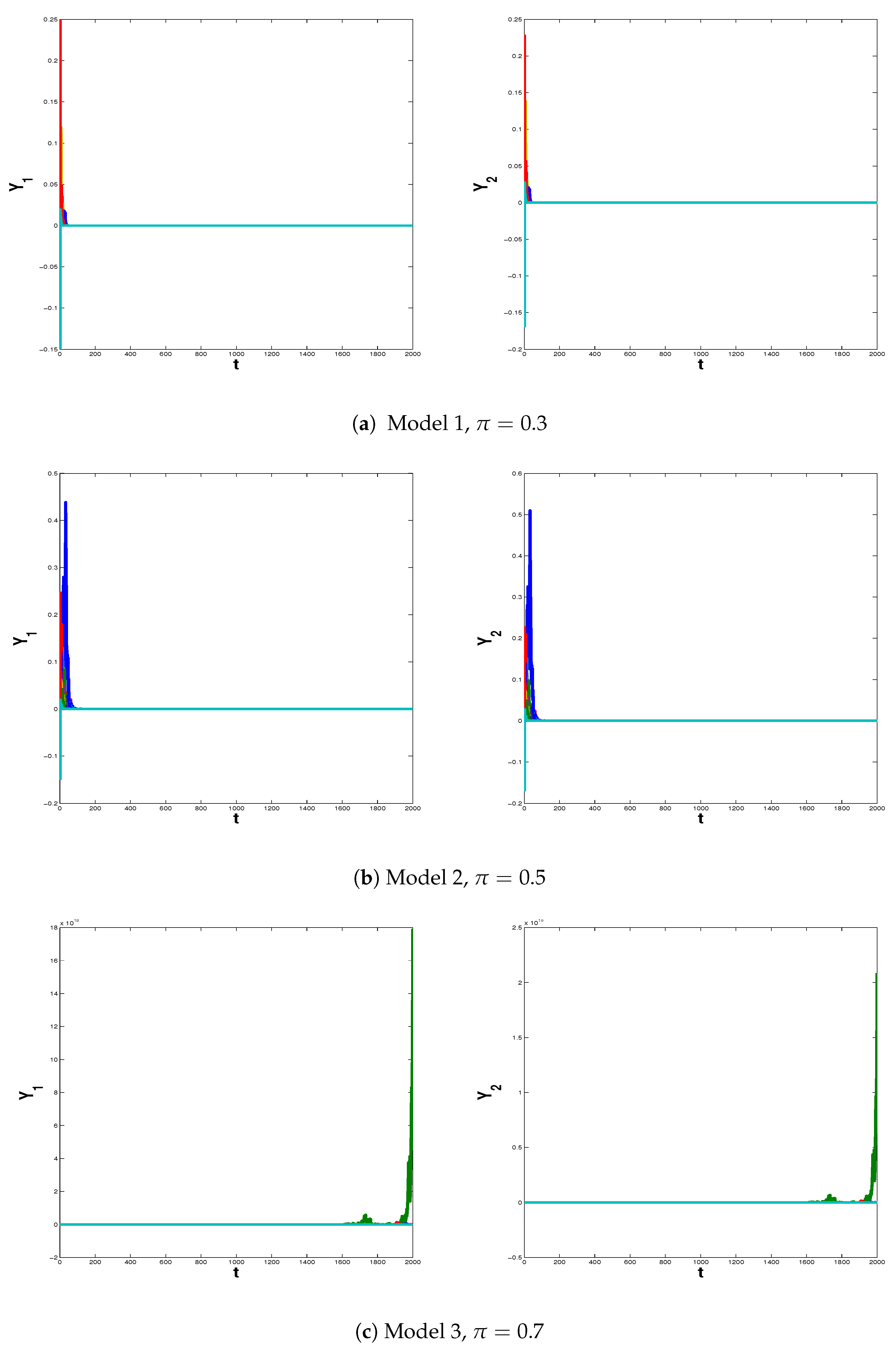
The parameter values used in the simulation study are shown in

Table 1. Parameter values used in simulating the bivariate TVAR model.

Group	Model	Regime 1, ${\mathsf{\Phi }}^1$		Regime 2, ${\mathsf{\Phi }}^2$		Probability of Regime 2, $\mathit{\pi }$	${\mathit{\lambda }}_{\mathit{max}}$
1	1	0.2	0.3	0.3	0.8	0.3	0.72
		0.3	0.4	0.5	0.8
	2	0.2	0.3	0.3	0.8	0.5	0.95
		0.3	0.4	0.5	0.8
	3	0.2	0.3	0.3	0.8	0.7	1.18
		0.3	0.4	0.5	0.8
2	4	0.2	0.3	1.1	1.2	0.1	0.84
		0.3	0.4	1.2	1.05
	5	0.2	0.3	1.1	1.2	0.3	1.8
		0.3	0.4	1.2	1.05
	6	0.2	0.3	1.1	1.2	0.5	2.8
		0.3	0.4	1.2	1.05
3	7	0.9	0.05	0.3	0.8	0.1	0.95
		0.7	0.3	0.2	0.8
	8	0.9	0.05	0.3	0.8	0.3	0.99
		0.7	0.3	0.2	0.8
	9	0.9	0.05	0.3	0.8	0.5	1.03
		0.7	0.3	0.2	0.8

Notes: This table shows the parameter values used in the simulated TVAR models. The distribution of the regimes is Bernoulli with probability to be in regime 2 equal to $\pi$. Notice that regime 2 is not stable in any of the models. In the right-hand column, we report the maximum eigenvalue of the matrix $(1-\pi ){\Phi }^1\otimes {\Phi }^1+\pi {\Phi }^2\otimes {\Phi }^2$, ${\lambda }_{max}$.

. As the table shows, regime 2 is by construction always (locally) explosive and we vary the value of $\pi$, the probability of regime 2, such that the overall TVAR model can be stationary or non-stationary. This is indicated by the maximum eigenvalue of the matrix $(1-\pi ){\Phi }^1\otimes {\Phi }^1+\pi {\Phi }^2\otimes {\Phi }^2$, which is reported in column six labelled ${\lambda }_{max}$. In particular, we define three groups of models, such that models within each group have the same coefficient matrices, but the probability to be in the explosive regime 2, $\pi$, varies.

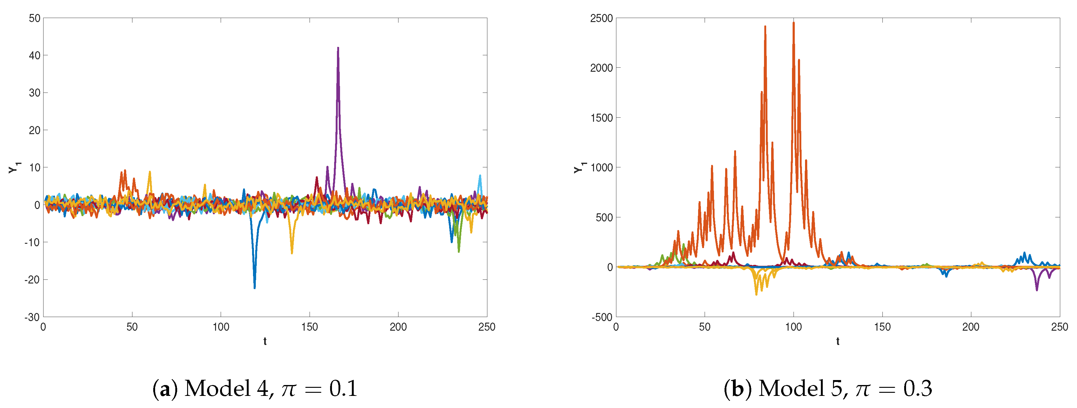
Models 1–6 are more strongly related to lags in the explosive regime 2 than in regime 1. We contrast our models such that the persistence of the models in the second regime is stronger in group 2 than group 1. When the second regime is mildly explosive, like the models from group 1, this regime has to occur very frequently, in order to make the whole TVAR model non-stationary. In contrast, model 6 is unstable even when the probability to be in the explosive regime is as low as 30%. This confirms numerically that, when one regime is not stable, the distribution of the regimes is crucial for the stationarity of the whole TVAR model.

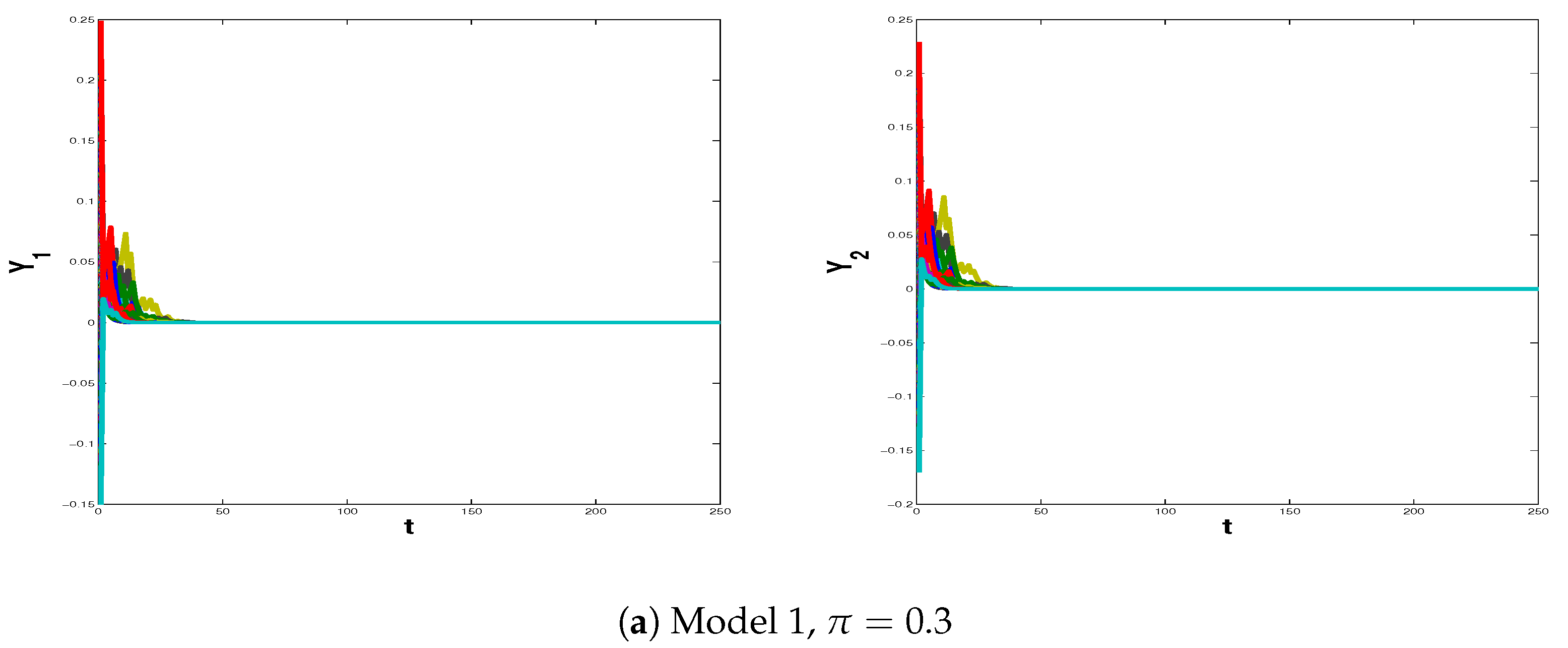
Figure 1 shows the simulated paths from models 1–3. When $\pi$ is fairly low (Panel a), the time series appear stationary. When $\pi$ gets larger and $\lambda$ is closer to 1, the simulated model looks like a unit root (Panel b). While models 1 and 2 generate spikes, the simulated series return to the initial level all the time, a characteristic of stationary processes. When $\pi =0.7$ (Panel c), the series is no longer stable and this is also evident from the figure. This conclusion is also valid when $n=2000$ (see Figure A1 in Appendix B).

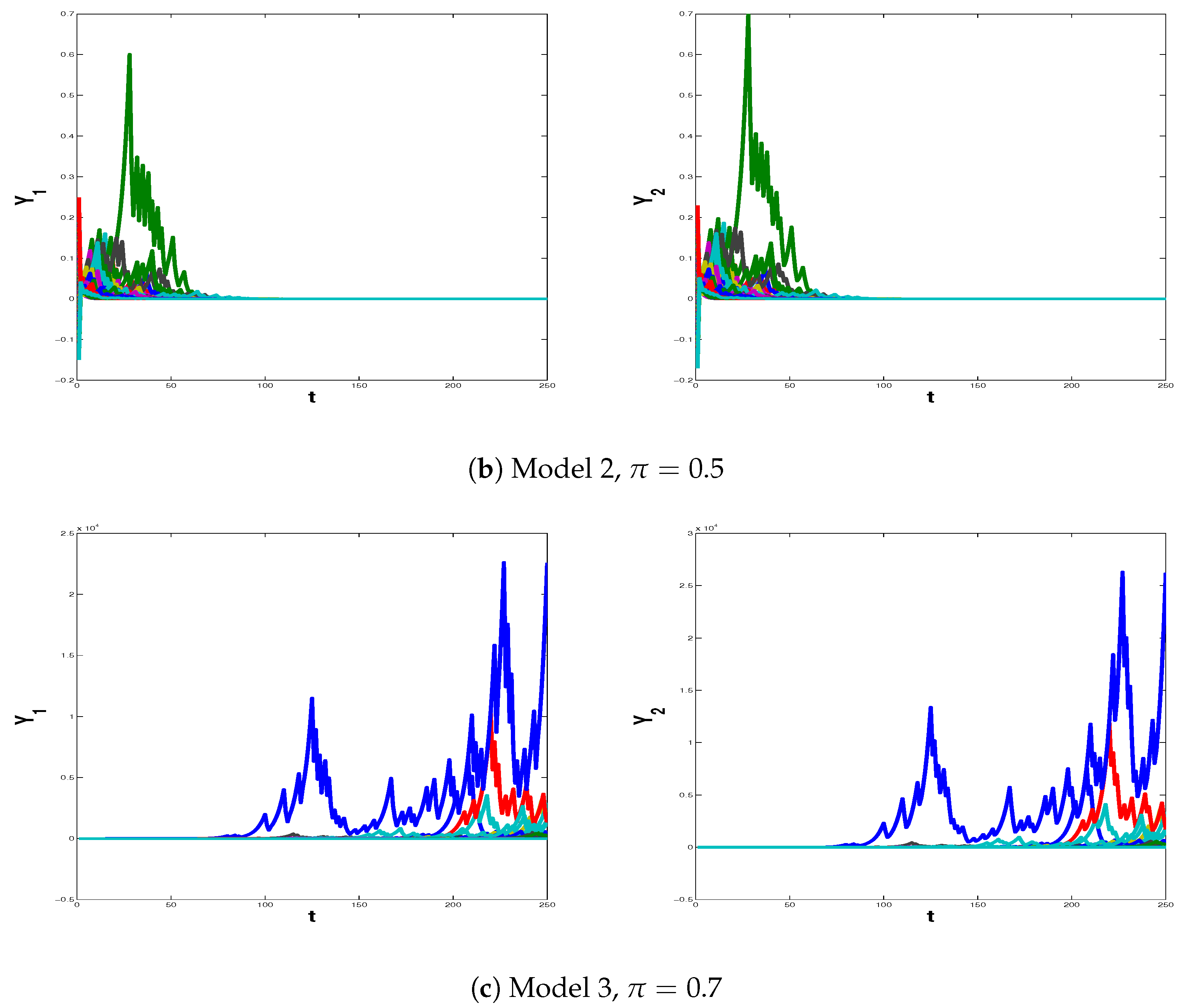
Figure 2 shows the simulated paths from models 4–6. These models are very persistent in regime 2 and they can generate huge spikes even when the probability of this regime is low (Panels a and b). Both models 4 and 5 look like unit root models, which explode, though they return to the initial level afterwards. Thus, the simulation exercise cannot reject stability of model 5, even though it is non-stationary by construction. The simulation study though does reject stability of model 6, when the probability to be in the explosive regime increases to 50% (Panel c). Thus, the results of the simulation might be misleading about non-stationary TVAR model with low probability of the explosive regime. The result of the simulation of models 4–6 prevails when $n=2000$ (see Figure A2 in Appendix B). It is of course impossible to check all starting points in a simulation study and we might simply not be lucky enough to have a starting point that allows rejecting stability of the model.

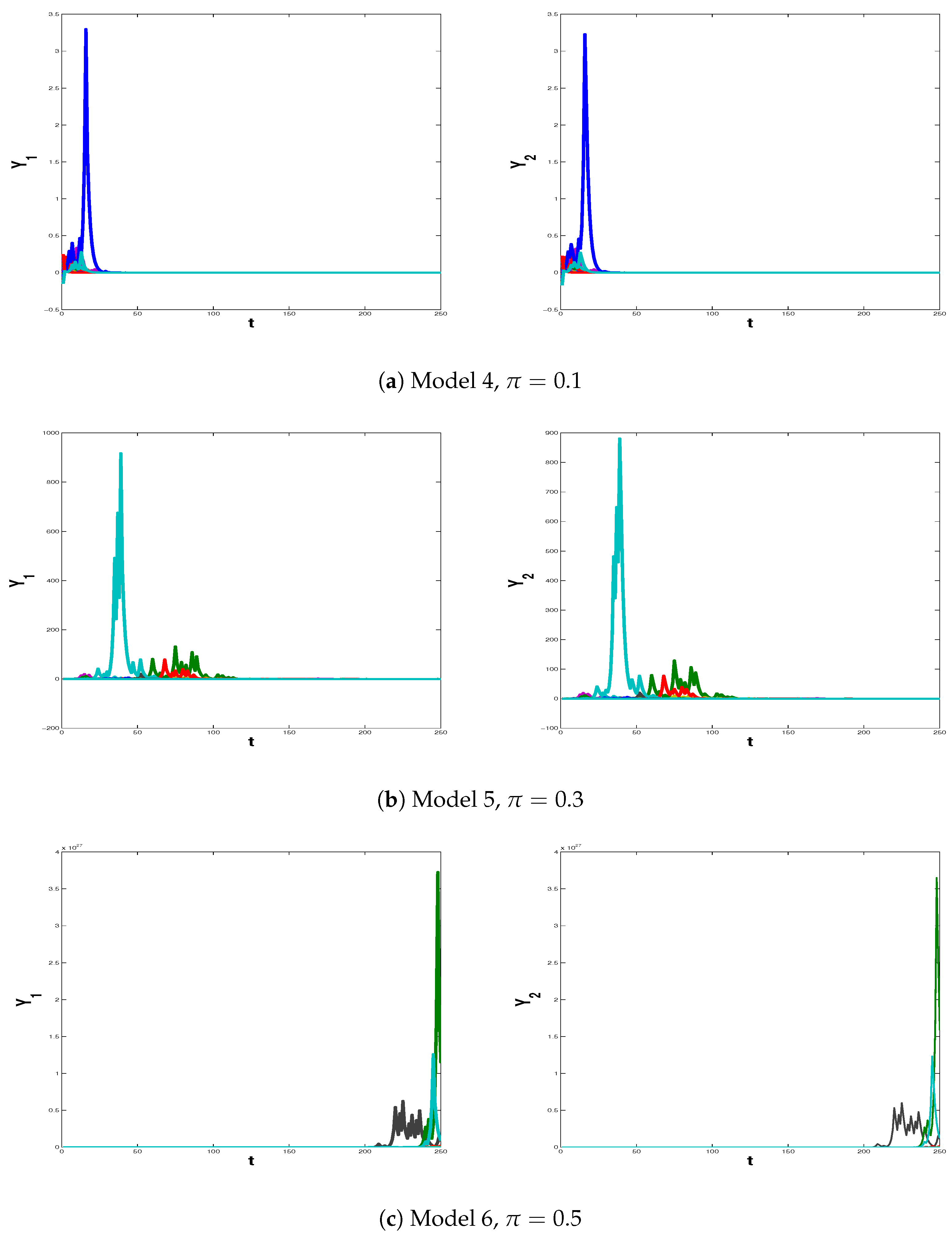
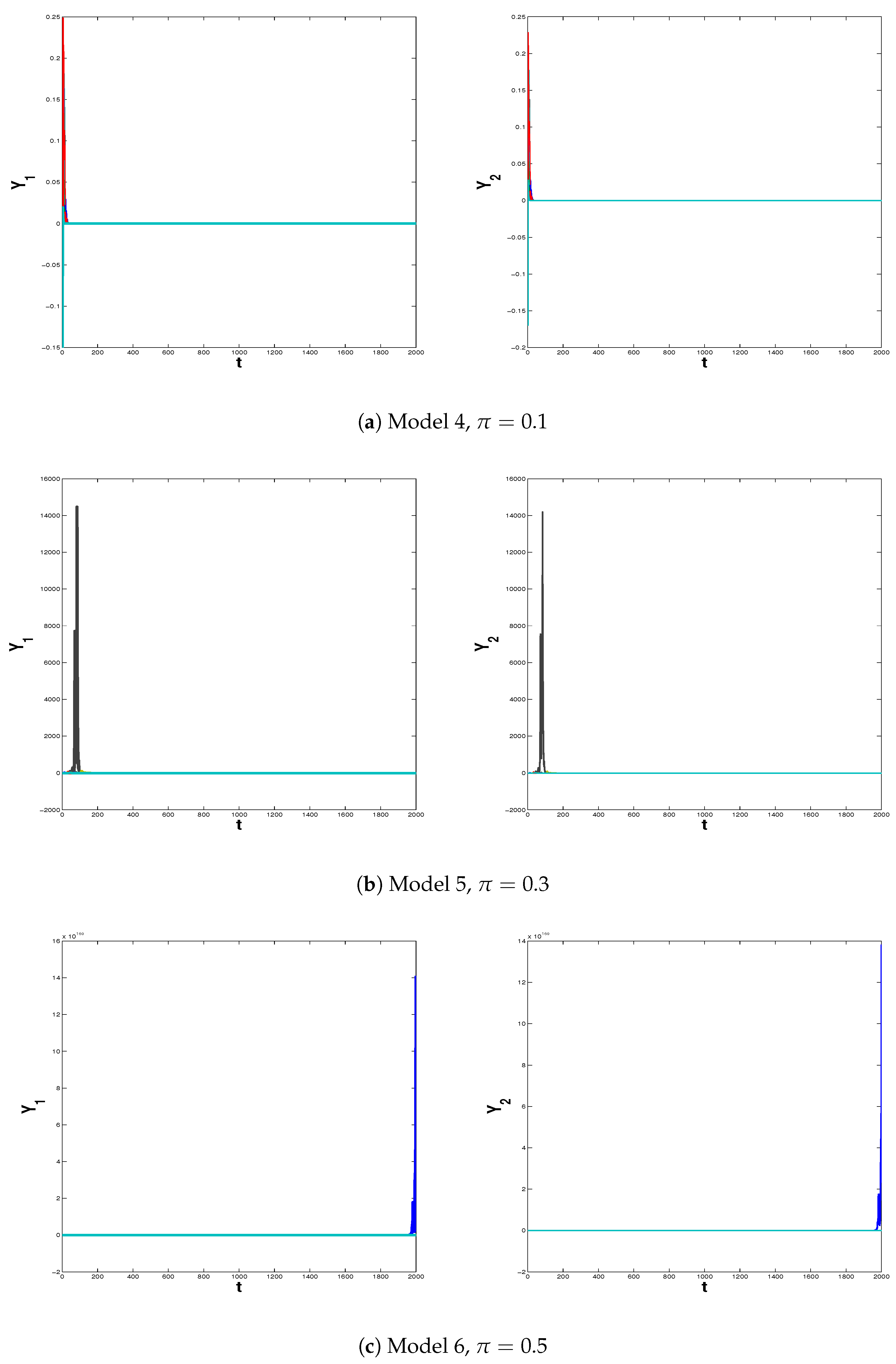
Models 7–9 describe a type of relationship, where a particular time series is more strongly related with its own lag in regime 1 and with the other time series in regime 2. These models are quite persistent in regime 1, but still remain stationary in this regime. Figure 3 shows the simulated paths from these models. The explosive performance of model 9 is evident from Panel c. The conclusion, however, is not clear about model 8. This model is quite persistent in both regimes, thus it can generate growing series, like those shown in Panel b, and simulation of model 8 may in fact lead to rejecting the stability of a stationary model. However, we cannot reject stability of the model when $n=2000$ (Panel b of Figure A3 in Appendix B). In fact, when the length of the simulated time series is increased to $n=2000$, the series from model 8 grows first but then returns to the initial level later on. Thus, the results from simulating model 8 show that the conclusion from this type of simulation study may also be sensitive to the sample size used in the simulation.

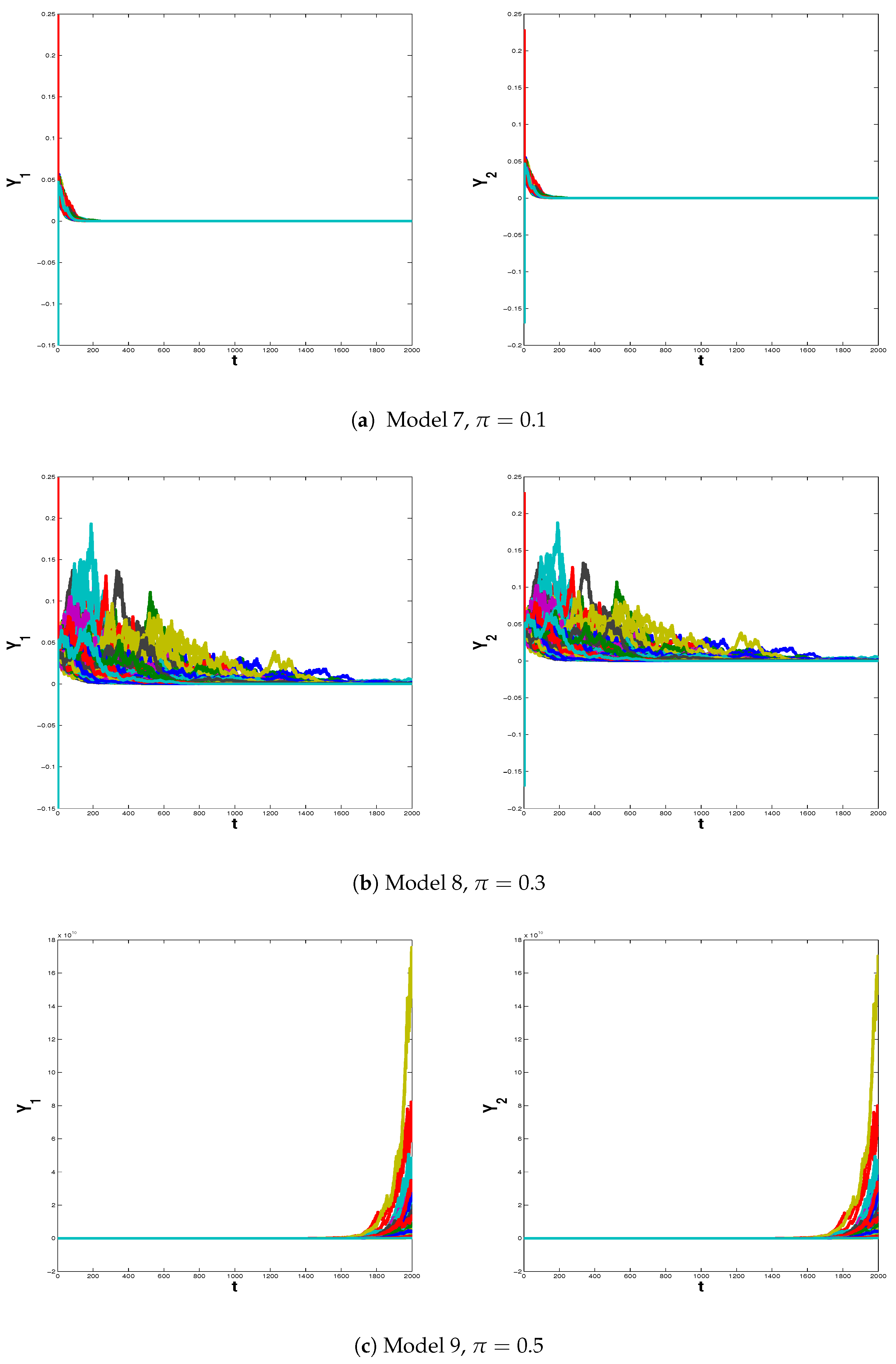
Figure 4 shows the simulated $Y_{1t}$ from TVAR models 4 and 5 specified in Table 1. We end this section by noting that the simulated series of $Y_t$ shown could be associated with data generating processes of financial or economic bubbles. Evans (1991) defines periodically collapsing explosive processes of bubbles such that the explosive behaviour of this process prevails through the whole sample, with non zero probability to collapse when it faces some threshold level. Phillips and Yu (2011) suggest a locally explosive process of bubbles, where asset prices transit from a unit root regime to an explosive regime and claim that this approach is consistent with other propagation mechanisms in financial markets like rational bubbles, exuberant responses to economic fundamentals and herd behaviour. Our simulation exercise shows that a simple bivariate locally explosive yet globally stationary TVAR model can generate unit root or explosive behaviour, which is consistent with these existing definitions of bubbles. An open question in the literature relates to how one can test for bubbles. In a recent paper, Ahmed and Satchell (2018) examine the performance of the Generalized Sup Augmented Dickey Fuller test proposed by Phillips et al. (2015) for the detection of explosive roots in univariate TAR models. They show that the power of the test drops considerably even though locally explosive regimes continue to be present when the process has a stationary distribution. We conjecture that this conclusion generalizes to the multivariate setting used in our paper.

4. Conclusions

This paper derives the necessary and sufficient conditions for the existence of a stationary distribution of the TVAR model with two regimes, when the regime process follows a Bernoulli distribution. These results are, to the best of our knowledge, unavailable in the existing literature. We further derive a closed form solution for the stationary distribution in the special case when there is no autoregressive structure in one of the regimes.

When the variables of interest are positively related, we describe a bivariate TVAR model, which is explosive in one regime, but allows for a stationary distribution along with finite moments. These results are related to so-called locally explosive models and our results extend the notion of locally explosive univariate processes to the bivariate case. We show that such models may remain stationary and, to ensure this, there is a trade-off between the persistence in a given regime and the probability of this regime.

In an empirical application, we simulate from various bivariate TVAR models, which are explosive in one of the regimes. We show how these models can capture the unit root and explosive behaviour, usually implied by the literature on bubble formation. We also demonstrate that a simulation study may fail to reject the stability of non-stationary TVAR models, when the probability of the explosive regime is low.