Nonparametric Estimation of a Conditional Quantile Function in a Fixed Effects Panel Data Model

1
Department of Economics, Texas A&M University, College Station, TX 77845, USA
2
International School of Economics and Management (ISEM), Capital University of Economics and Business, Beijing 100070, China
*
Author to whom correspondence should be addressed.
J. Risk Financial Manag. 2018, 11(3), 44; https://doi.org/10.3390/jrfm11030044
Submission received: 11 July 2018
/
Revised: 31 July 2018
/
Accepted: 1 August 2018
/
Published: 3 August 2018
(This article belongs to the Special Issue Nonparametric Econometric Methods and Application)
Abstract
:This paper develops a nonparametric method to estimate a conditional quantile function for a panel data model with an additive individual fixed effects. The proposed method is easy to implement, it does not require numerical optimization and automatically ensures quantile monotonicity by construction. Monte Carlo simulations show that the proposed estimator performs well in finite samples.
JEL Classification:
C14; C211. Introduction
Using nonparametric techniques to estimate econometric models has received increasing attention among econometricians in recent decades (see, for example, Pagan and Ullah (1999); Hall et al. (2007); Belloni et al. (2016); Lin et al. (2015); Li et al. (2013); Firpo et al. (2009) and Firpo et al. (2018) for the literature of nonparametric methods and applications). The most popular nonparametric model is the conditional mean regression model. However, compared with a conditional mean function, a conditional quantile regression function, when evaluated at different quantiles, can reveal an entire distributional relationship between the covariates and the response variable. Quantile regression therefore has many useful applications in economics and finance. For example, in risk and financial management, researchers are more concerned about the uncertainty or the risk of an asset, which can be characterized by its left tail behavior (corresponding to the lower quantiles) (see Al Rahahleh and Bhatti (2017); Al Rahahleh et al. (2017); Nguyen and Bhatti (2015); Al Rahahleh et al. (2016); Bartram et al. (2018); Al Shubiri and Jamil (2018) for the literature on idiosyncratic risk), and quantile regression can play an important role in this line of research.
The existing work on nonparametric estimation of quantile functions mostly focuses on cross-sectional data, or weakly dependent stationary data processes. Nonparametric estimation of conditional quantile functions with panel data is more difficult when there exists fixed effects term that is correlated with covariates. In this paper, we consider the following nonparametric panel data model with individual fixed effects:
where is the outcome variable, is a scalar1, is the individual fixed effect, it has zero mean and is allowed to be correlated with in an unknown correlation form, is smooth but otherwise unspecified function, the idiosyncratic error is with zero mean and a finite variance. Given that has a zero mean, we have from Equation (1) that . Without loss of generality, we assume that .2
A key attractive feature of panel data for empirical researchers is that it controls for the unobserved heterogeneity. Equation (1) has been discussed in Henderson et al. (2008), with a focus on the nonparametric estimation and testing of the conditional mean function. Our interest lies in estimating the conditional quantile function of given . The application of quantile regression to panel data framework has been a challenging task (see, for example, Koenker (2004); Abrevaya and Dahl (2008); Kato et al. (2012); Harding and Lamarche (2014)). The check-function method and inverse-CDF method are the two main methods in quantile regression analysis, with the former most widely used in literature. One main challenge with the check-function method is that the objective criterion function is non-differentiable and therefore numerical optimization is required. This creates a computational burden. Another drawback of the check-function method is the lack of monotonicity, also known as the quantile crossing problem (see Bassett and Koenker (1982) and He (1997)). Researchers often need to impose shape restrictions or use monotone rearrangement to address the quantile crossing problem (Chernozhukov et al. (2010); Qu and Yoon (2015)).
This paper develops a new quantile regression method for the nonparametric panel data Equation (1) in the spirit of Fang et al. (2018)3. The new method exploits the location-scale structure of Equation (1). Note that the conditional -th quantile function of given , denoted by , takes a particularly simple closed-form structure:
for all , where is the -th quantile of 4. Thus, if is the estimator of , then can be estimated by
where is the empirical quantile function of the (normalized) regression residuals.
For estimation, we first use the first-difference transformation to get rid of the individual fixed effect and estimate the the unknown function by the series method, we then use deconvolution method to back up the distribution of error term , therefore the quantile estimator of . Finally, we exploit the location-scale structure of the first-differenced model to derive the quantile estimator of , which is given in Equation (3). The deconvolution step closely relates to the papers by Horowitz and Markatou (1996) and Evdokimov (2010) for the application of the deconvolution method to recover the density of panel data error term. Our approach does not require numerical optimization, is computationally easy to implement, and automatically ensures quantile monotonicity by construction. For asymptotic property of the conditional quantile estimator, as long as the series estimator and are consistent 5, the conditional quantile estimator is also consistent by Equation (3) and the continuous mapping theorem. While we do not provide theoretical underpinnings for the proposed quantile estimator, Monte Carlo simulation results show that the estimator performs well in finite samples.
The remainder of the paper is organized as follows. Section 2 gives a detailed description of the methodology. Section 3 presents a Monte Carlo simulation to examine the finite-sample performance of the proposed quantile estimator. Section 4 considers an extension where the error is heteroskedastic. Section 5 concludes the paper.
2. Methodology
In this section, we describe the three-step procedure to estimate the conditional quantile function .
STEP 1.
Use the first-difference to get rid of individual fixed effects and estimate by the nonparametric series method.
First differencing Equation (1), we have that
Note that despite if one uses a de-mean dependent variable or not, it leads to the same first-differenced Equation (4) because any additive constant will be wiped out by first-difference transformation.
Let denote the dimensional basis functions, where K is the number of basis functions. For example, we may choose power series base function so that , or we can choose spline base function. By the approximation property of series basis function, there exists an vector of constants such that as , where is a compact support of . In practice, one can estimate by the least squares method based on
where , , , and .
We estimate by applying the OLS to Equation (5), yielding that
where is an matrix of base functions, is an matrix, is an vector of outcome variables, and is an vector.
We therefore obtain the series estimator of :
STEP 2.
Let denote the density of . In this step, we use the deconvolution method to recover .
From Step 1, one can obtain the estimator of by .
To see how the density of can be estimated, let and denote the characteristic functions of and , respectively, where . Assume that the distribution of is such that is real and positive for all . Then, it is easy to see that
where in the third equality we use the independence of and , and the fourth equality uses the symmetry of .
Therefore,
We propose the following steps to obtain the density estimate of :
STEP 3.
We estimate by such that for , satisfies the following condition:
Therefore, for , the -th conditional quantile estimator of , given , is estimated by
where and are estimated in Steps 1 and 2, respectively.
Remark 1.
In Step 1, the consistency estimation of requires that as , and . In series estimation, plays a role similar to the bandwidth h in kernel methods. In practice, one can use Mallows’s or leave-one-out cross-validation method to determine the series term K. We refer readers to Li and Racine (2007) for details.
Remark 2.
Note that, in Step 2, assuming is real and is equivalent to assuming that the density of is symmetric around 0. We are using the assumption that is positive in deriving Equation (6).
Remark 3.
In Step 2, the smoothing parameter depends on the sample size . To guarantee that uniformly converges to over at a geometric rate with respect to the sample size n, Hu and Ridder (2010) suggests that we can choose such that
where is a constant.
Remark 4.
For inference, we recommend using a residual bootstrap method similar to Fang et al. (2018). We leave the proof of validity of such a bootstrap procedure to a future research topic.
3. Monte Carlo Simulation
In this section, we conduct Monte Carlo simulations to assess the performance of the proposed conditional quantile estimator.
We consider the following data generating process (DGP):
where , where is , is . We consider two distributions for : (i) is ; (ii) is (a t-distribution with degree of freedom 3).
We conduct 2000 Monte Carlo replications for samples of size with . We report mean squared error (MSE) of three estimators: (1) the series estimator with , (2) the quantile estimator with , and (3) the conditional quantile estimator with . For each of the three quantities above, we average them over the 2000 replications.
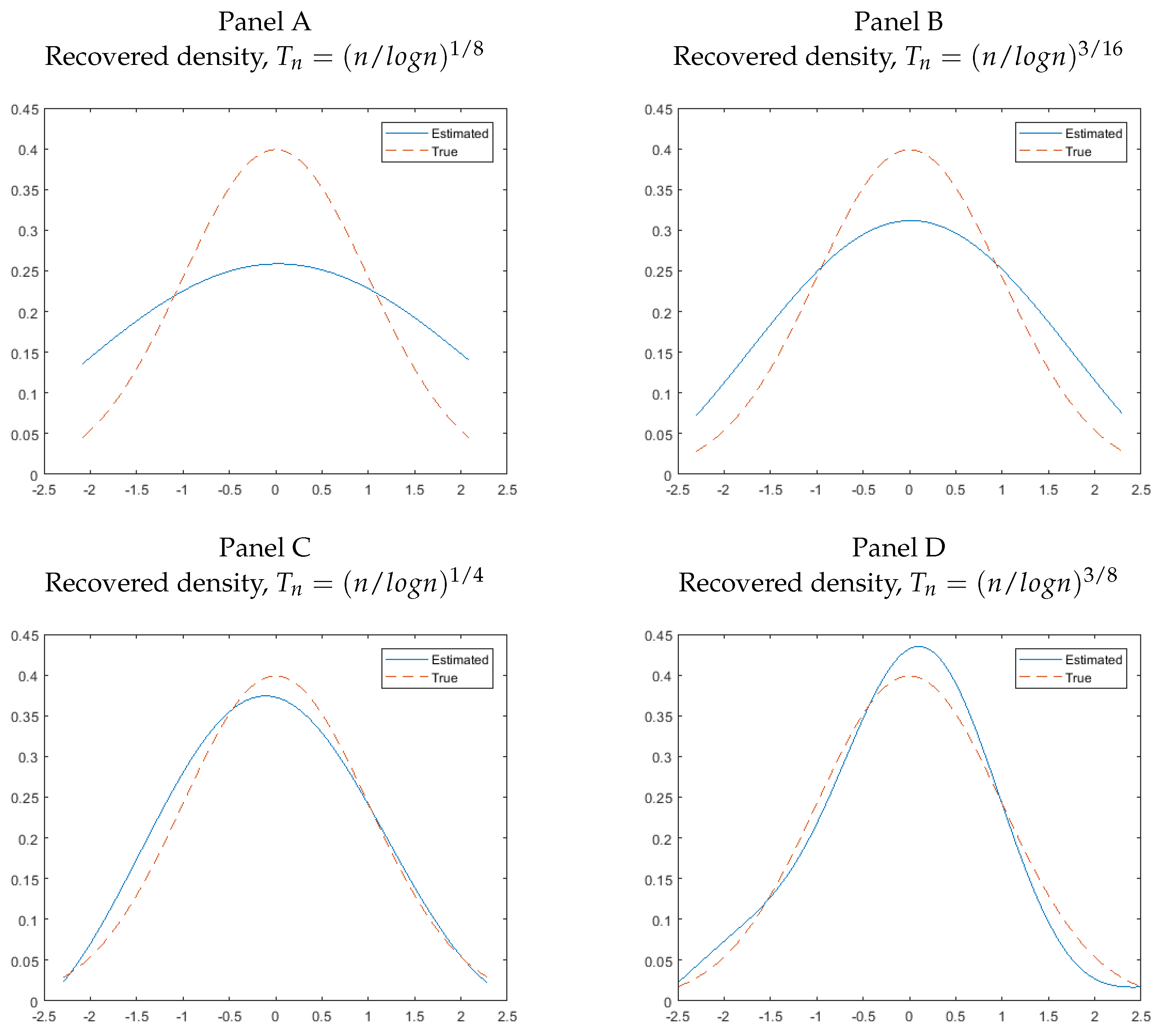
We first examine the performance of the deconvolution method for recovering the density of error terms. As an illustration, we only present the result (Figure 1) for the case of , with sample size . We examine the sensitivity of the estimated density to the choice of different bandwidths. We set , and . It can be seen from Figure 1 that the performance of the deconvolution method can be somewhat sensitive to the choice of bandwidth. This is a well known problem of the deconvolution method, not a particular problem to our approach. When is small, say , the estimated density is flatter than the true density. However, generally, the estimated density tracks the true density6.
4. Extension: Conditional Heteroskedastistic Error Case
In this section, we consider an extension where the error term is conditional heteroskedastic. Specifically, we generalize Equation (1) to the following case7:
where is an unknown function, is assumed to be with zero mean, unit variance and independent of . Without loss of generality, we assume that (similar to the conditional homoskedasticity case).
Define . The conditional -th quantile function of given , denoted by , takes the following closed-form structure:
for all , where , and is the (un-conditional) -th quantile of .
Remark 5.
In deriving Equation (10), we use the fact that because and and are independent with each other.
Remark 6.
Noting that, due to the independence between and , we have that , and this implies that (conditional independence property).
We propose the following three-step procedure to estimate the conditional quantile function of given .
STEP 1.
We obtain by exactly the same procedure as in Step 1 of the conditional homoskedastic error case.
STEP 2.
We use the deconvolution method to estimate , the conditional density of given . Define . Assuming that the density of is symmetric around zero,8 and note that , we have
where , the third equality uses the conditional independence property as described in Remark 6, and in the fourth equality we use the symmetry of , and is symmetric around zero.
Under the assumption that is positive, the above equation implies that . The left-hand side of Equation (11) can be estimated from data:
Therefore, we estimate by . Let denote the conditional density of given . Then, using the deconvolution method as in the homoskedastic case, one can recover using as in Equation (8). We use to denote the resulting estimator of .
STEP 3.
Let denote the estimate of , . The following identity
suggests that we can obtain based on the following equation:
where is estimated from Step 2.
By Equation (10), the -th conditional quantile estimator of , given , is estimated by
where is obtained in Step 1, and is obtained in Step 3.
Remark 7.
Note that, in the last step, we estimate the τ-th quantile of directly, instead of estimating the unknown function and separately (e.g., Fang et al. (2018)).
5. Conclusions
In this paper, we propose an easy-to-implement nonparametric method to estimate conditional quantile functions in a fixed effects panel data model. There are many directions that one can extend the results of this paper to more general settings. For example, one can allow for panel non-stationary data as considered in Chen and Khan (2008) or allow for the covariate to be endogenous. We leave these as possible future research topics.
Author Contributions
The two authors both contribute to the project formulation and paper preparation.
Funding
This research received no external funding.
Acknowledgments
We thank three anonymous referees for helpful and constructive comments.
Conflicts of Interest
The authors declare no conflict of interest.
References
- Abrevaya, Jason, and Christian M. Dahl. 2008. The effects of birth inputs on birthweight. Journal of Business & Economic Statistics 26: 379–97. [Google Scholar]
- Al Rahahleh, Naseem, Iman Adeinat, and M. Ishaq Bhatti. 2016. On ethnicity of idiosyncratic risk and stock returns puzzle. Humanomics 32: 48–68. [Google Scholar] [CrossRef]
- Al Rahahleh, Naseem, and M. Ishaq Bhatti. 2017. Co-movement measure of information transmission on international equity markets. Physica A: Statistical Mechanics and its Applications 470: 119–31. [Google Scholar] [CrossRef]
- Al Rahahleh, Naseem, M. Ishaq Bhatti, and Iman Adeinat. 2017. Tail dependence and information flow: Evidence from international equity markets. Physica A: Statistical Mechanics and its Applications 474: 319–29. [Google Scholar] [CrossRef]
- Al Shubiri, Faris Nasif, and Syed Ashsan Jamil. 2018. The impact of idiosyncratic risk of banking sector on oil, stock market, and fiscal indicators of Sultanate of Oman. International Journal of Engineering Business Management, 10. [Google Scholar] [CrossRef]
- Bartram, Söhnke M., Gregory W. Brown, and René M. Stulz. 2018. Why Has Idiosyncratic Risk Been Historically Low in Recent Years? National Bureau of Economic Research Working Paper NO. 24270. Cambridge, MA, USA: National Bureau of Economic Research, January. [Google Scholar]
- Bassett, Gilbert, Jr., and Roger Koenker. 1982. An empirical quantile function for linear models with iid errors. Journal of the American Statistical Association 77: 407–15. [Google Scholar] [CrossRef]
- Belloni, Alexandre, Victor Chernozhukov, and Ivan Fernández-Val. 2016. Conditional quantile processes based on series and many regressors. arXiv, arXiv:1105.6154. [Google Scholar]
- Chen, Songnian, and Shakeeb Khan. 2008. Semiparametric estimation of nonstationary censored panel data models with time varying factor loads. Econometric Theory 24: 1149–73. [Google Scholar] [CrossRef]
- Chernozhukov, Victor, Iván Fernández-Val, and Alfred Galichon. 2010. Quantile and probability curves without crossing. Econometrica 78: 1093–25. [Google Scholar]
- Evdokimov, Kirill. 2010. Indentification and Estimation of a Nonparametric Panel Data Model with Unobserved Heterogeneity. Working Paper. Princeton, NJ, USA: Princeton University. [Google Scholar]
- Fang, Zheng, Qi Li, and Karen Yan. 2018. A Simple Nonparametric Method for Estimation and Inference of Conditional Quantile Functions. Working Paper. Available online: https://ssrn.com/abstract=3223015 (accessed on 3 August 2018).
- Firpo, Sergio, Nicole M. Fortin, and Thomas Lemieux. 2009. Unconditional quantile regressions. Econometrica 77: 953–73. [Google Scholar]
- Firpo, Sergio P., Nicole M. Fortin, and Thomas Lemieux. 2018. Decomposing wage distributions using recentered influence function regressions. Econometrics 6: 28. [Google Scholar] [CrossRef]
- Hall, Peter, Qi Li, and Jeffrey S. Racine. 2007. Nonparametric estimation of regression functions in the presence of irrelevant regressors. The Review of Economics and Statistics 89: 784–89. [Google Scholar] [CrossRef]
- Harding, Matthew, and Carlos Lamarche. 2014. Estimating and testing a quantile regression model with interactive effects. Journal of Econometrics 178: 101–13. [Google Scholar] [CrossRef]
- He, Xuming. 1997. Quantile curves without crossing. The American Statistician 51: 186–92. [Google Scholar]
- Henderson, Daniel J., Raymond J. Carroll, and Qi Li. 2008. Nonparametric estimation and testing of fixed effects panel data models. Journal of Econometrics 144: 257–75. [Google Scholar] [CrossRef] [PubMed]
- Horowitz, Joel L., and Marianthi Markatou. 1996. Semiparametric estimation of regression models for panel data. The Review of Economic Studies 63: 145–68. [Google Scholar] [CrossRef]
- Hu, Yingyao, and Geert Ridder. 2010. On deconvolution as a first stage nonparametric estimator. Econometric Reviews 29: 365–96. [Google Scholar] [CrossRef]
- Kato, Kengo, Antonio F. Galvao, and Gabriel V. Montes-Rojas. 2012. Asymptotics for panel quantile regression models with individual effects. Journal of Econometrics 170: 76–91. [Google Scholar] [CrossRef]
- Koenker, Roger. 2004. Quantile regression for longitudinal data. Journal of Multivariate Analysis 91: 74–89. [Google Scholar] [CrossRef]
- Li, Qi, Juan Lin, and Jeffrey S. Racine. 2013. Optimal bandwidth selection for nonparametric conditional distribution and quantile functions. Journal of Business & Economic Statistics 31: 57–65. [Google Scholar]
- Li, Qi, and Jeffrey Scott Racine. 2007. Nonparametric Econometrics: Theory and Practice. Princeton: Princeton University Press. [Google Scholar]
- Lin, Wei, Zongwu Cai, Zheng Li, and Li Su. 2015. Optimal smoothing in nonparametric conditional quantile derivative function estimation. Journal of Econometrics 188: 502–13. [Google Scholar] [CrossRef]
- Nguyen, Cuong, and M. Ishaq Bhatti. 2015. Investor sentiment and idiosyncratic volatility puzzle: Evidence from the chinese stock market. Journal of Stock and Forex Trading 4: 2. [Google Scholar]
- Pagan, Adrian, and Aman Ullah. 1999. Nonparametric Econometrics. Cambridge: Cambridge University Press. [Google Scholar]
- Qu, Zhongjun, and Jungmo Yoon. 2015. Nonparametric estimation and inference on conditional quantile processes. Journal of Econometrics 185: 1–19. [Google Scholar] [CrossRef] [Green Version]
| 1. | For ease of exposition, we assume is univariate, the extension to multivariate case can be carried over straightforwardly. |
| 2. | This can be achieved by using de-mean data for the dependent variable, i.e., replacing by in Equation (1). For notational simplicity, we still use to denote the dependent variable although it is actually the de-mean version of it. |
| 3. | Recently, Fang et al. (2018) proposes a new nonparametric method for estimating a conditional quantile function with cross-sectional data. We refer readers to Fang et al. (2018) for a detailed discussion. |
| 4. | For ease of exposition, we drop the subscript in and use to denote the -th quantile of in general, since is an sequence. |
| 5. | The consistency can be straightforwardly shown using similar arguments as in Fang et al. (2018) and Horowitz and Markatou (1996). |
| 6. | There is no rule-of-thumb to choose the optimal bandwidth in the deconvolution method. In practice, researchers can try different bandwidths as a robust check to see how results vary across the different bandwidths. |
| 7. | Fang et al. (2018) also considers the same form of heteroskedastic error as described here. |
| 8. | This implies the conditional density of given is symmetric, since, given that , the symmetry of is equivalent to the symmetry of . |
Figure 1.
Recovered densities across different bandwidths and homoskedastic symmetric normal errors.
Figure 1.
Recovered densities across different bandwidths and homoskedastic symmetric normal errors.

Table 1.
Mean MSE (×100), Errors.
| Sample Size | Estimators | ||||||
|---|---|---|---|---|---|---|---|
| 0.0149 | 0.0037 | 0.0022 | 0.0006 | 0.0204 | 0.0185 | 0.0163 | |
| 0.0092 | 0.0012 | 0.0007 | 0.0002 | 0.0107 | 0.0102 | 0.0096 | |
| 0.0048 | 0.00051 | 0.00028 | 0.000082 | 0.0052 | 0.0050 | 0.0048 | |
Table 2.
Mean MSE (×100), Errors.
| Sample Size | Estimators | ||||||
|---|---|---|---|---|---|---|---|
| 0.0139 | 0.0423 | 0.0235 | 0.0065 | 0.0642 | 0.0433 | 0.0235 | |
| 0.0094 | 0.0210 | 0.0128 | 0.0036 | 0.0304 | 0.0222 | 0.0130 | |
| 0.0048 | 0.0091 | 0.0063 | 0.0019 | 0.0104 | 0.0112 | 0.0067 | |
© 2018 by the authors. Licensee MDPI, Basel, Switzerland. This article is an open access article distributed under the terms and conditions of the Creative Commons Attribution (CC BY) license (http://creativecommons.org/licenses/by/4.0/).
Share and Cite
MDPI and ACS Style
Yan, K.X.; Li, Q. Nonparametric Estimation of a Conditional Quantile Function in a Fixed Effects Panel Data Model. J. Risk Financial Manag. 2018, 11, 44. https://doi.org/10.3390/jrfm11030044
AMA Style
Yan KX, Li Q. Nonparametric Estimation of a Conditional Quantile Function in a Fixed Effects Panel Data Model. Journal of Risk and Financial Management. 2018; 11(3):44. https://doi.org/10.3390/jrfm11030044
Chicago/Turabian StyleYan, Karen X., and Qi Li. 2018. "Nonparametric Estimation of a Conditional Quantile Function in a Fixed Effects Panel Data Model" Journal of Risk and Financial Management 11, no. 3: 44. https://doi.org/10.3390/jrfm11030044