1. Introduction
Analyzing the relationship between the environment and health has become a major issue for public health in France as forecasted by the national plans for health and environment (NPHE). Two priority areas were selected during the first NPHE: (1) preventing health risks related to the quality of resources and to chemicals and (2) developing environmental health through research, expertise, training and information. In 2009, the second NPHE was prepared from the perspective of the upcoming conference on health and the environment organized by the World Health Organization. Two main axes were prioritized: (1) identifying and managing geographic areas where hotspot exposures to substances present in air, soil, water, and foods resulting from anthropic activities suspected of generating potentially increasing risks to human health and (2) reducing environmental health inequalities. Thus, environmental health inequality has become a substantial topic that guides policy developments in France. To address this aim, there is an urgent need for tools that can quantify the spatial relationships between the environment, socioeconomics and health and that can highlight areas with strong inequalities.
Health inequalities are a quite recent study topic. Previous studies were essentially based, at an individual level, on specific surveys [
1,
2] and, at a spatially aggregated level (administrative unit), on specific regions [
3,
4]. At a regional scale, data are often available at a fine level or resolution. This allows for building environmental, socioeconomic and health indicators at different spatial scales; for example, Salmond
et al. [
5] built a new census-based index of deprivation based on the smallest possible geographical areas.
Regarding health data, there are strict privacy rules for individual-level health data that prohibit their public release. Aggregated data are only available at the geographic level, from which disclosure and reconstruction of patient identity are impossible. In France these census units could be regions or counties. This aggregation unfortunately results in incidence or mortality rates that can be unreliable over small and/or sparsely populated areas. This effect, known as the “small number problem” [
6], should be corrected for an accurate evaluation of health-environment relationships.
Several authors have already addressed the spatial relationships between health data and environmental data. One of the issues faced by spatial epidemiologists and for exposure assessment is the combination of data measured for very different spatial scales and with different levels of reliability. In reality, the analysis of cancer mortality maps is often hindered by the presence of noise caused by unreliable extreme rates computed from sparsely populated geographic units. A number of approaches have been developed to improve the reliability of risk estimates [
7,
8]. The most commonly used are Bayesian methods [
9], which are commonly referred to as the BYM model. Bayesian methods prohibit any change of scales, an operation that is easily conducted within the framework of kriging. Goovaerts and Gebreab [
10] conducted a simulation-based evaluation of the performance of geostatistical and full Bayesian disease-mapping models, and they found that the geostatistical approach yielded smaller prediction errors and more precise and accurate probability intervals and that it allowed for better discrimination between counties with high and low mortality risks.
Poisson kriging, in this context, presents a spatial methodology that allows for filtering the noise caused by the small number problem and enables the estimation of mortality risk and the associated uncertainty at different spatial scales. This approach has been implemented to modeling cancer risk by a number of authors: Oliver
et al. [
11] studied cases of cancer in children under fifteen years of age, and Goovaerts and collaborators considered lung cancer [
12,
13], breast cancer [
14,
15], prostate cancer [
16], cervical cancer [
17], and pancreatic cancer [
18], and all found it to be relevant for this particular problem.
Selection of scale is perhaps the most important factor in creating and analyzing a relationship between environmental exposure and health outcomes [
19]. This issue is similar to the modifiable area unit problem (MAUP), a term introduced by Openshaw [
20,
21]. The MAUP can cause differences in the analytical results of the same input data compiled under different zoning systems [
22,
23].
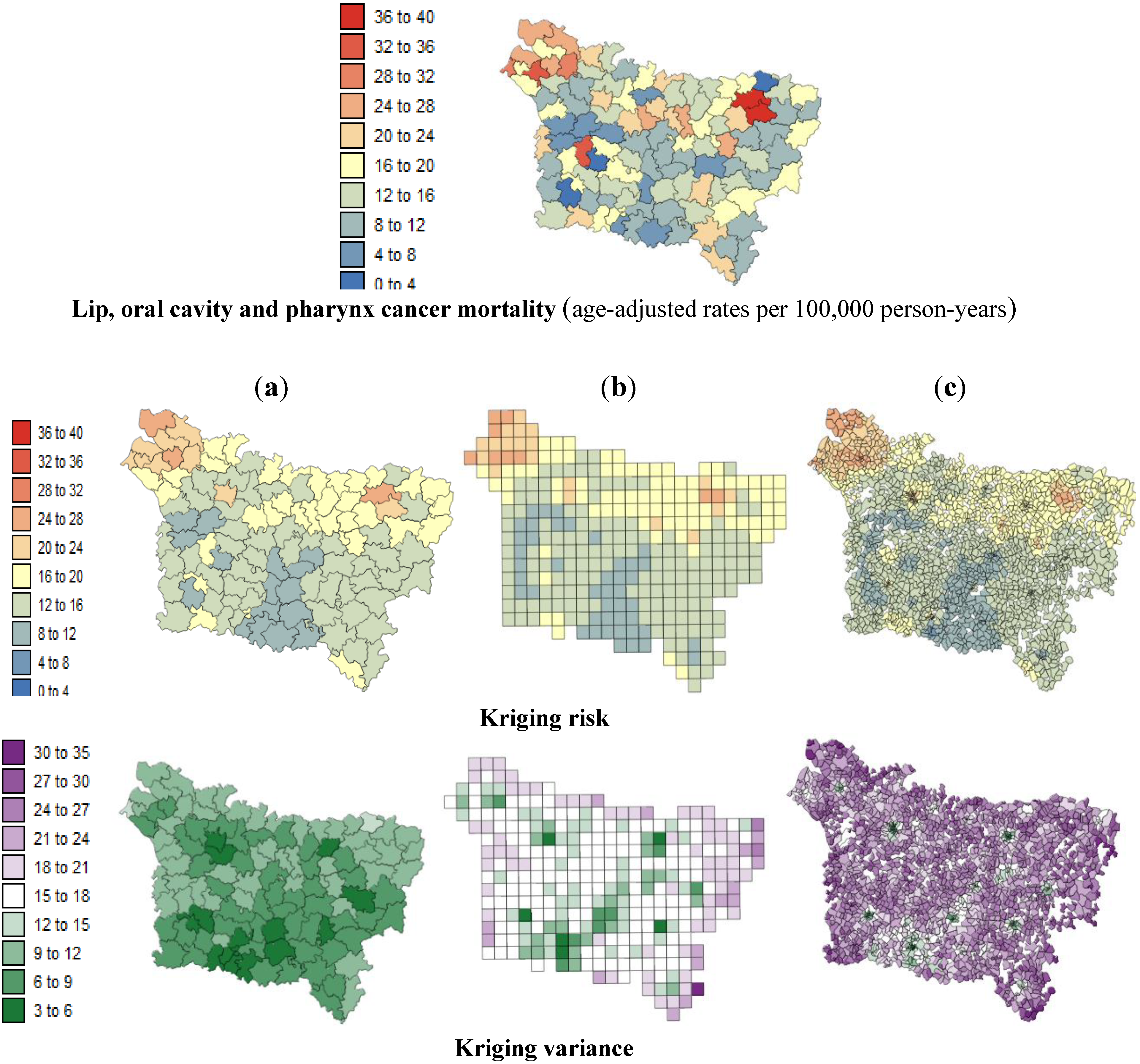
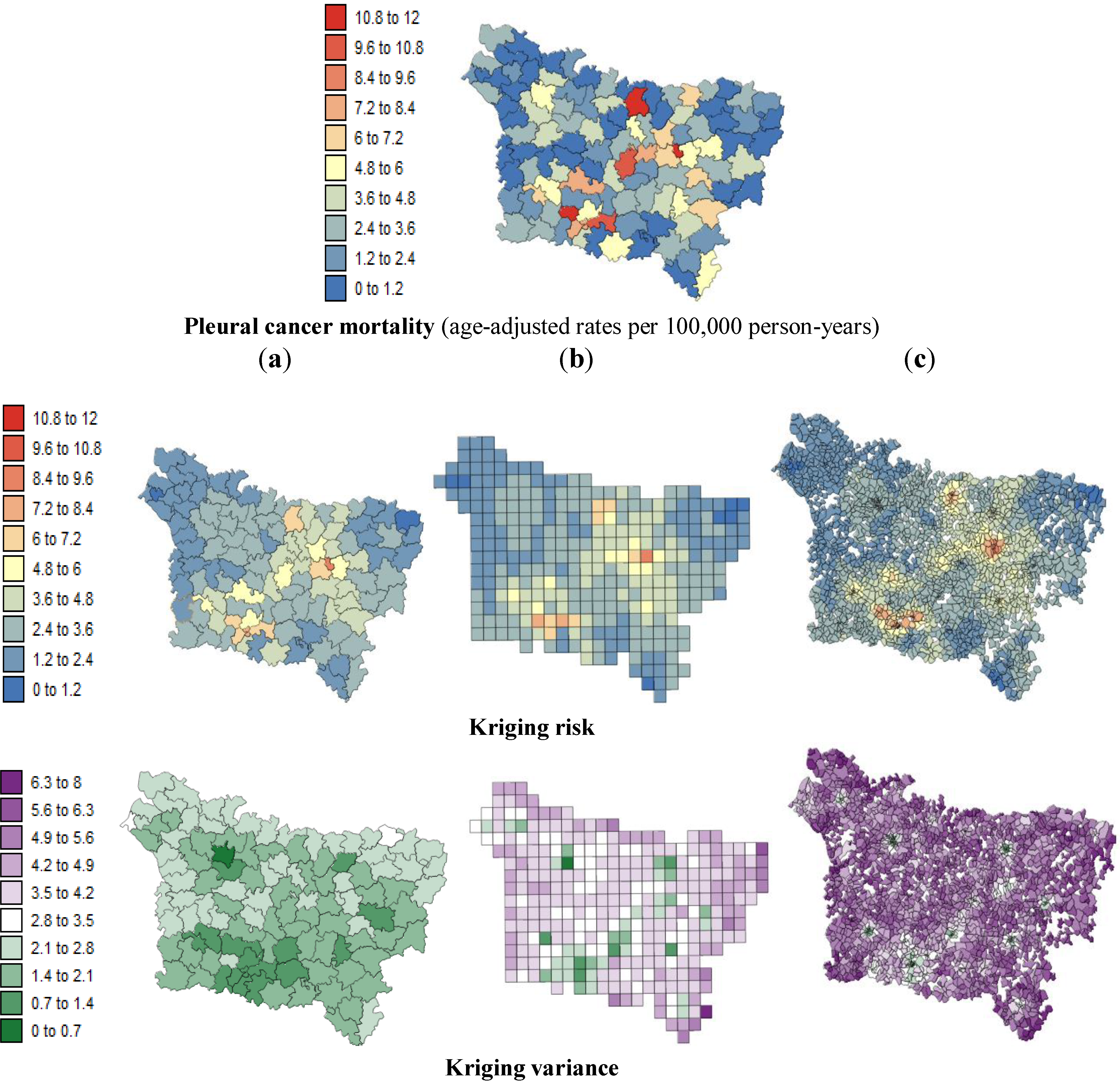
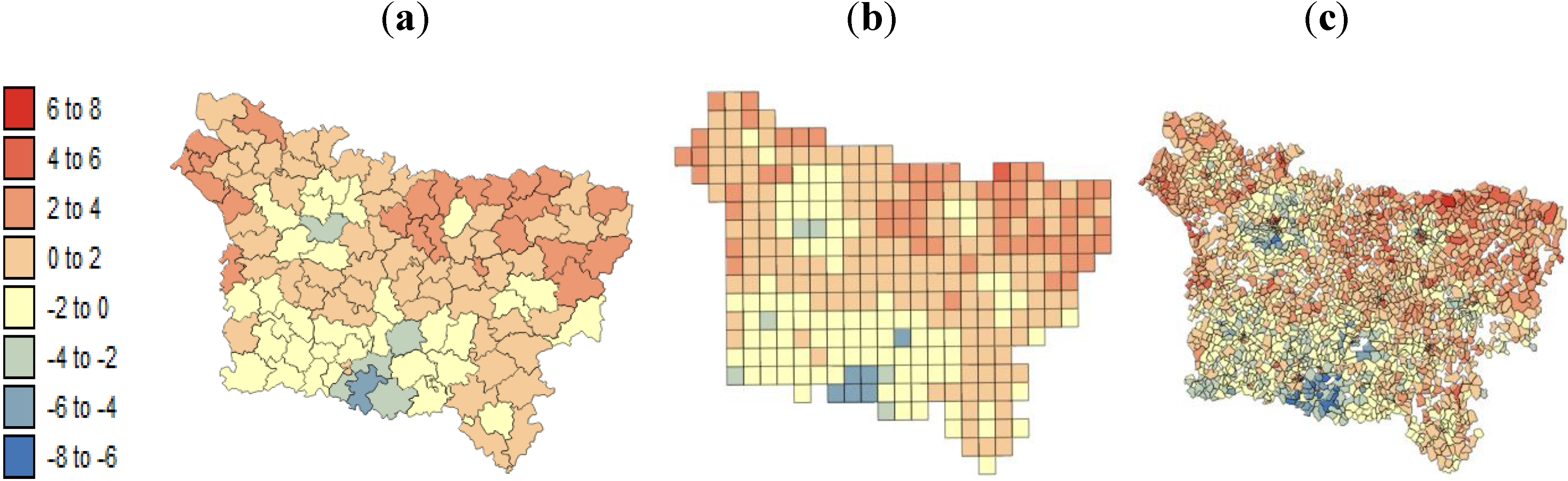
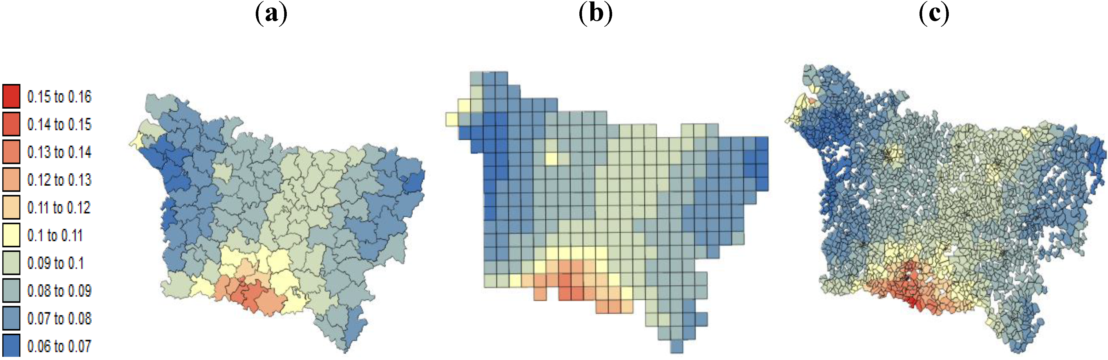
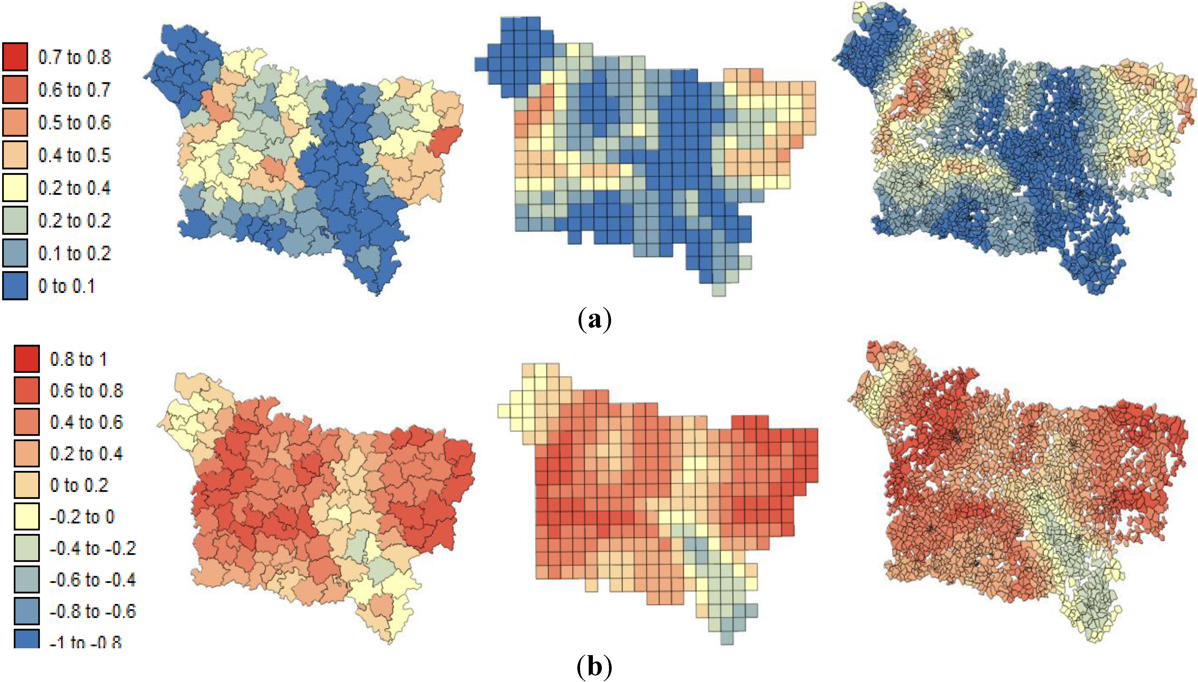
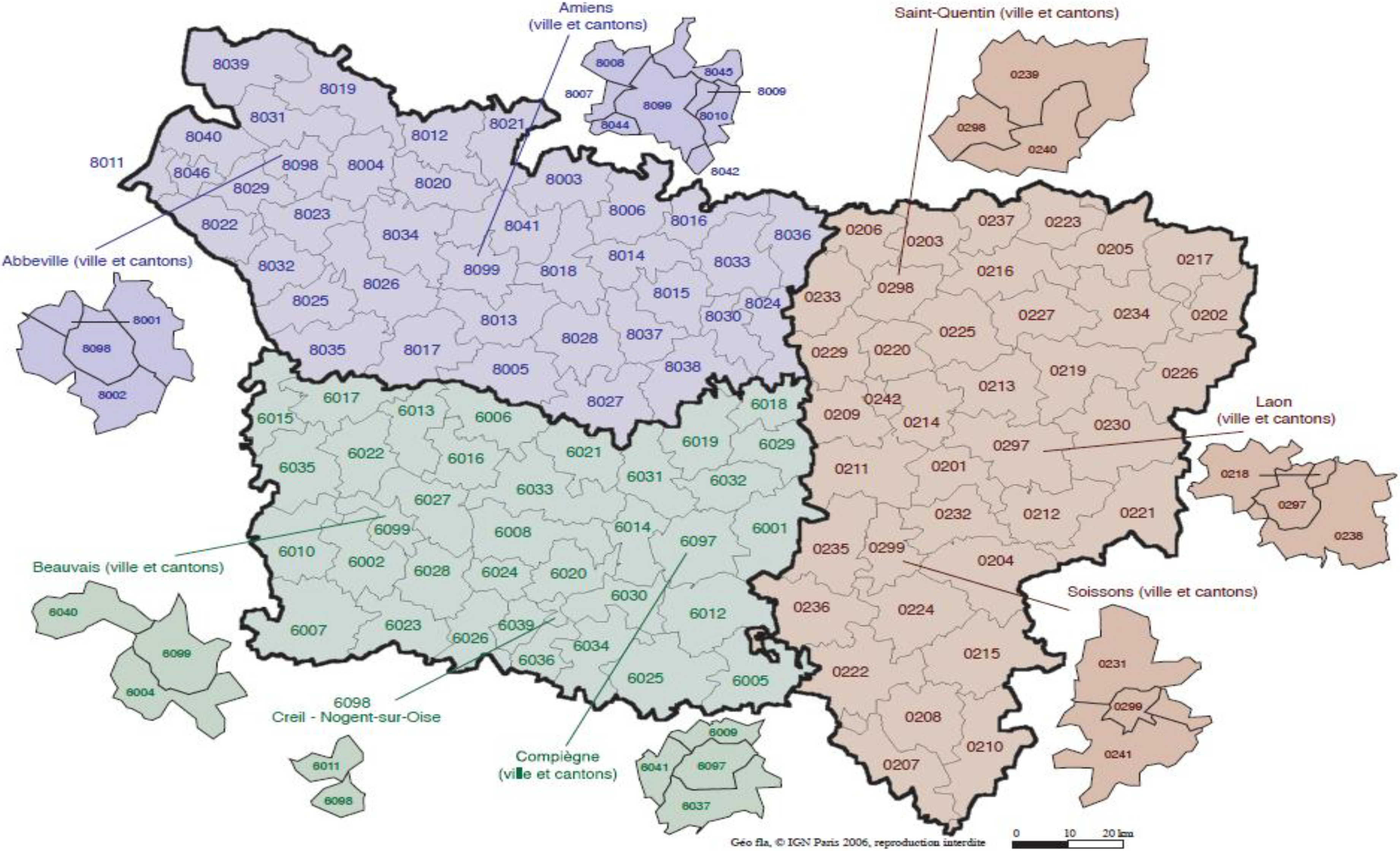
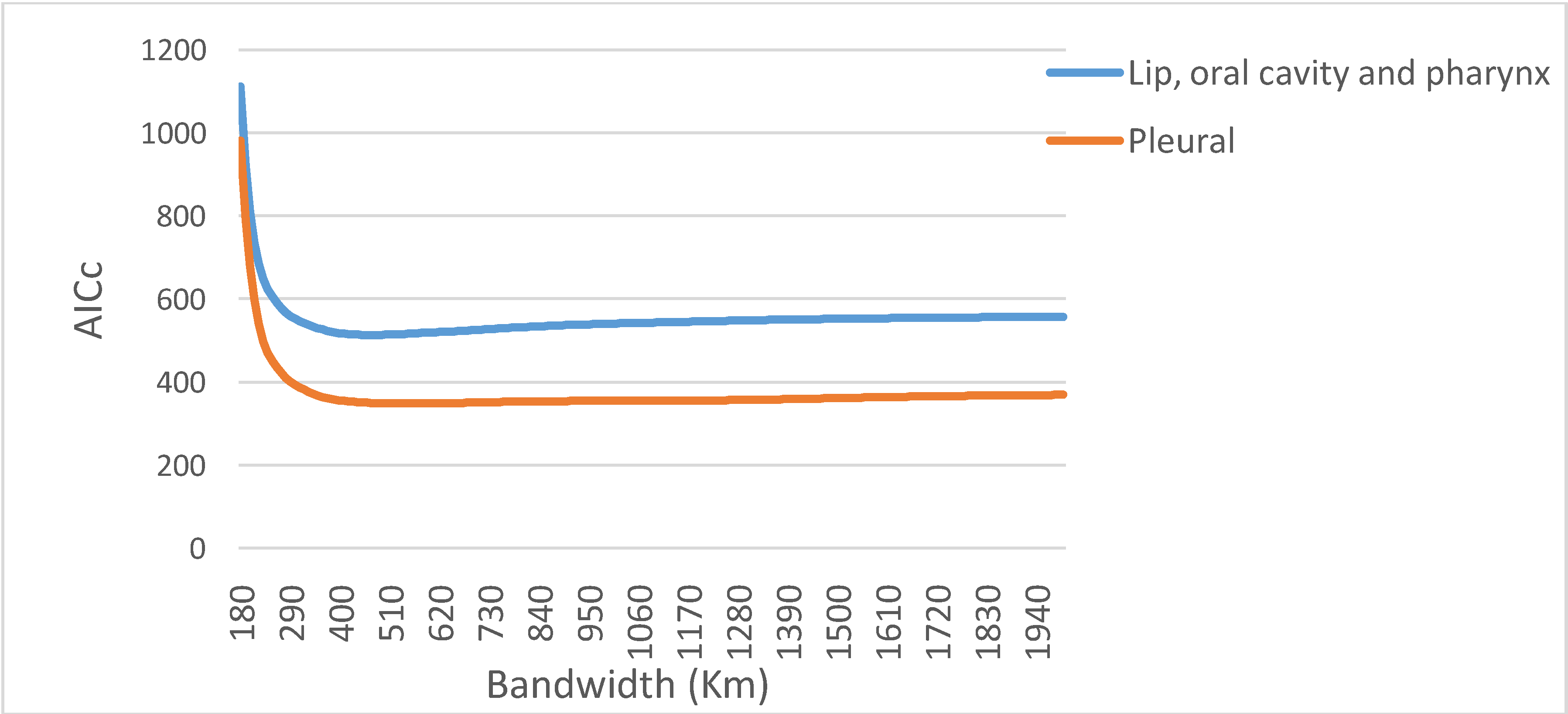
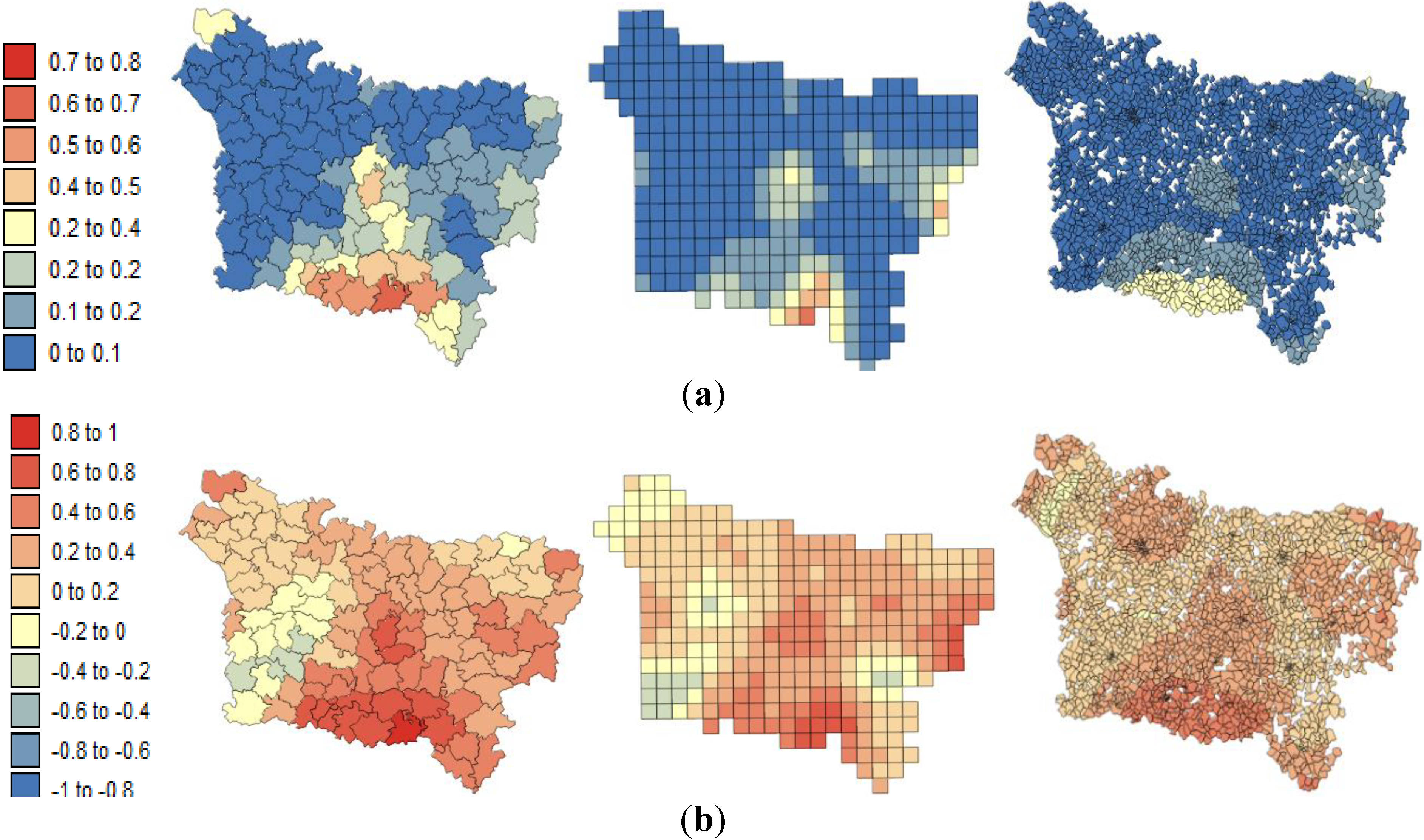
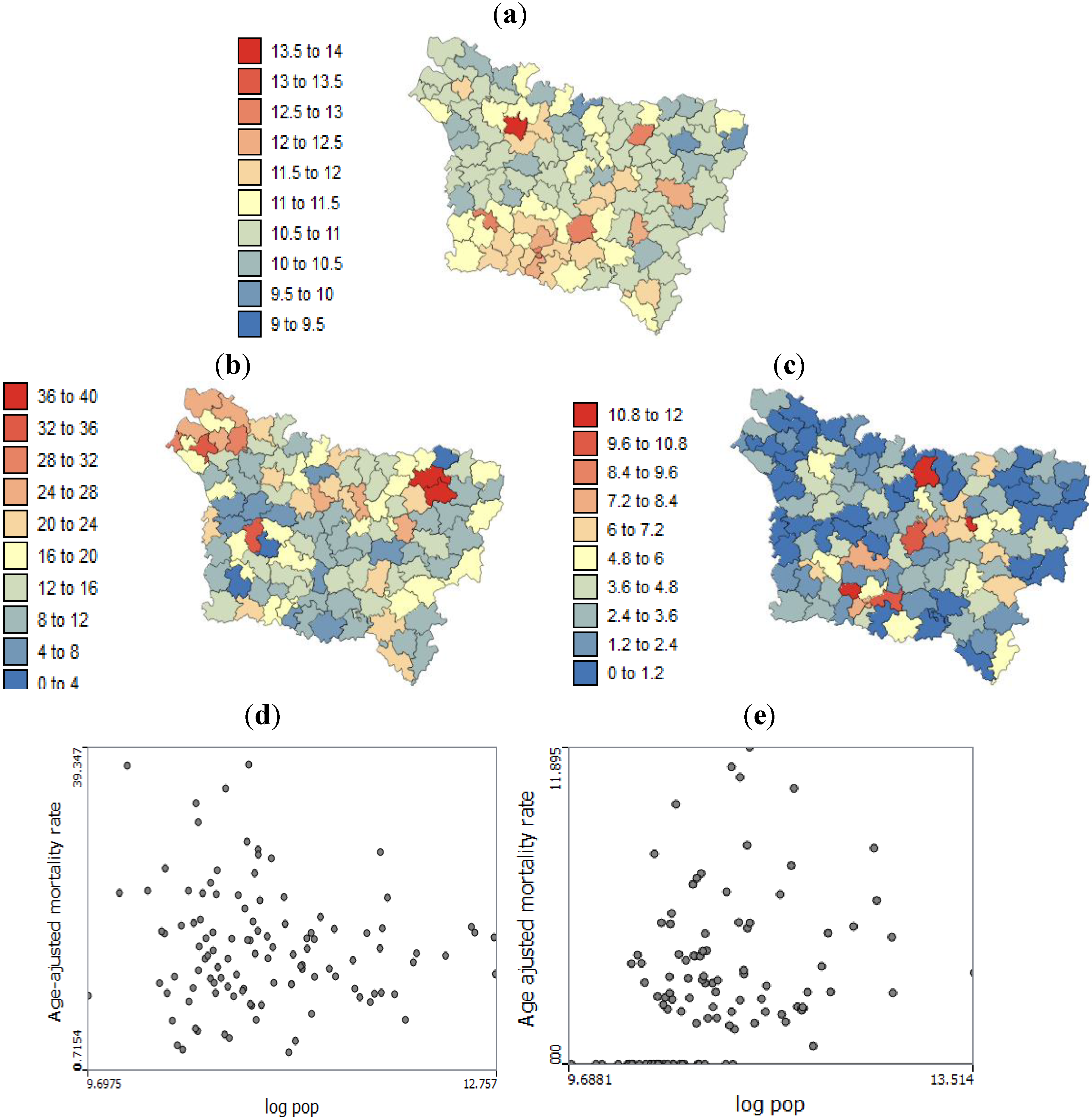
The present study aims to evaluate spatial relationships at three levels of aggregation: the IRIS level, an intermediate scale (the grid level), and the county level between health outcomes (mortality attributable to cancer) initially aggregated to the county level, district socioeconomic covariates, and exposure data modeled on a regular grid. The approach is illustrated using age-adjusted lip, oral cavity and pharynx, and pleural cancer mortality rates over the period 2000–2009 for the Picardy region. The deprivation index and trace metal exposure indicators are used as putative risk factors.
4. Discussion
Our results substantiate the work on noise filtering described in the introduction section from Oliver
et al. [
11] and Goovaerts
et al. [
12,
18]. Indeed, we found the following: (1) the mean risk values estimated under each of the three spatial structures were similar; (2) the IRIS risk estimates were non-negative; (3) and their sums were equal to the original county risk. Although the disaggregation of cancer data on a small scale is somewhat arbitrary, in particular when it does not take into account secondary information to guide this downscaling, the approach should facilitate the analysis of the relationships between health data and the putative covariates (
i.e., environmental, socioeconomic, behavioral or demographic factors) that are typically estimated for different spatial scales. These covariates can potentially be subsequently used as secondary information in the kriging, leading to more detailed risk maps at finer scales [
42].
The other issue was the so-called modifiable areal unit problem (MAUP), for which different geographic scales can lead to inconsistent results for relationships analysis. For example, the mortality rate reported at (1) the county level requires an aggregated deprivation index at the same resolution, and this aggregation obscures the intra-county variation and thus the relationship and (2) the IRIS level, at which the disaggregation leads to a large variance in estimated risk. Exploratory methods, such as the univariate Moran’s can serve as indications of the potential effect of the MAUP in the study how relationships based on the homogeneity and heterogeneity of spatial data are affected by the study level and may affect the ability of the study to detect a relationship [
43].
In this study, very similar results were obtained for the different spatial scales between:
pleural cancer mortality and the exposure indicator F1.
lip, oral cavity, pharynx cancer mortality and the SE index.
Whereas other studies on the relationship between heath and deprivation showed that the use of spatial representations other than the census tract produced different analytical results [
35,
44], the significant association between lip, oral cavity, pharynx cancer mortality and the SE index estimated using the county structure were stronger than they were under the IRIS structure.
This difference between the significant correlation coefficients is the result of aggregation because the aggregation level is known to increase the strength of correlation [
20]. Future work could provide tools to exhaust all possible aggregations and generate empirical frequency distributions of the statistical estimates that could be used to evaluate the sensitivity of results to aggregation effects.
Based on the results obtained, we can confirm that the presence of this significant statistical association was likely not induced by the use of a particular geography. At the three spatial scales, the strongest correlation coefficients were found where low deprivation was associated with low lip, oral cavity and pharynx cancer mortality and where low environmental pollution was associated with low pleural cancer mortality.
5. Conclusions
This paper presents an approach for evaluating spatial relationships between health outcomes (mortality attributable to cancer) initially aggregated at the county level, district socioeconomic covariates, and exposure data modeled on a regular grid. The approach was illustrated using age-adjusted lip, oral cavity and pharynx, and pleural cancer mortality rates measured over the period 2000–2009 for the Picardy region. The deprivation index and trace metal exposure indicators were used as putative risk factors. For the different spatial scales, the strongest associations were found where low deprivation was associated with low lip, oral cavity and pharynx cancer mortality and where low environmental pollution was associated with low pleural cancer mortality. However, applying this approach to other areas, for other causes of death, or with other indicators always requires exploratory analysis to assess the role of the MAUP and downscaling health data in the study of the relationships that will allow decision-makers to develop interventions where they are the most needed.


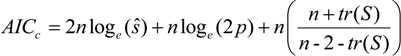
 is the estimate of the standard deviation of the residuals, and tr(S) is the trace of the hat matrix. For more information on the theory and practical application of GWR, the reader is referred to Fotheringham et al. [34].