1. Introduction
The cone-beam scanning configuration with a circular trajectory remains one of the most popular scanning configuration and has been widely employed for data acquisition in 3-D X-ray computed tomography (CT), because it allows for operating at a high rotating speed due to its symmetry, avoiding the need to axially translate the patient, such as in helical or step-and-shoot CT [
1,
2]. Unfortunately, a circular trajectory does not satisfy Tuy's data sufficiency condition [
3] which requires every plane that passes through the reconstruction region (ROI) must also cut the trajectory at least once and therefore only approximate reconstructions are possible. In the pursuit of the data sufficiency condition, various scanning trajectories have been proposed, such as circle and line [
4,
5], circle plus arc [
6,
7], double orthogonal circles [
8,
9] and dual ellipses [
10].
Recently, the FDK algorithm [
11] has been implemented for a cone-beam vertex trajectory consisting of three-orthogonal isocentric circles [
12]. On the other hand, we know that 3D image reconstruction based on three-orthogonal circular isocentric orbits is sufficient in the sense of Tuy data sufficiency condition. Therefore the datum obtained from three-orthogonal circular isocentric orbits can derive an exact reconstruction algorithm. In this paper, another theoretically exact and general inversion formula which was proposed in Katsevich [
13] will be implemented for three-orthogonal circular isocentric orbits. Compared with the aforementioned algorithms, the distinctive features of Katsevich's algorithm can be summarized as the choice of a more general weight and a novel way to dealing with discontinuous in weight. Furthermore, Katsevich's algorithm has been implemented for various scanning trajectories, such as circle and line [
14,
15], circle plus arc [
16], several circular segment [
17], two orthogonal circles [
13] and helix [
18,
19].
In contrast to a singular circular trajectory, there are several advantages in using weighted reconstruction with the three-orthogonal-circular trajectory. First, for the reconstruction noise due to the algorithm is ’trajectory’ dependent. Using three-orthogonal geometry with weighting function, the noise is suppressed. Second, the three-orthogonal setting yields better image quality in comparison with classical scheme for larger cone-angles. Last, the scan method for three-orthogonal geometry can be implemented with minimal requirements and can provide a better 3D reconstruction for small animals or objects. At the same time, compared to the two-circular trajectory, artifacts of the boundaries of the ROI where artifacts are likely to appear are suppressed by the additional filtering lines and according weighting functions.
In our implementation, a new weighting scheme is developed so that all measurements are used by accurately averaging over multiply measured projections of the three-orthogonal-circular scanning. Moreover, this new weighted reconstruction is differs from the weighted FDK [
11] reconstruction with the three-orthogonal-circular trajectory [
12] considerably, in that it is a theoretically exact formulation of a general shift invariant filtered back-projection (FBP) reconstruction framework. In this paper, we show the derivation of our cone-beam FBP reconstruction algorithm starting with Tuy's inversion formula. In other words, we discuss how to derive a FBP cone-beam reconstruction formula from the Tuy's classical inversion formula. To construct the reconstruction formula, several operators are needed. First, using some properties of the cone-beam transform, the classical Tuy's inversion formula can be written as (the first-order derivative of the Radon transform in ℝ
3) Grangeat's inversion formula [
20] in a weighted form. Then, using the methodology in[
13], we can get the final inversion formula. The features of our inversion formula can be summarized as follow: using some properties of the cone-beam transform to derive the inversion formula, a proper choice of the weighting function, deriving equations of the filtering lines and describing geometric properties of filtering lines in the planar detector plane.
The organization of this paper is as follows. In Section 2, we derive Katsevich's inversion formulation by Tuy's weighted form. In Section 3, we derive equations of the filtering planes and filtering lines. In Section 4, we show the geometric properties of filtering lines in the planar detector plane and according weighting functions.
3. Equation of Filtering Lines for the Three-Orthogonal Circular Scanning
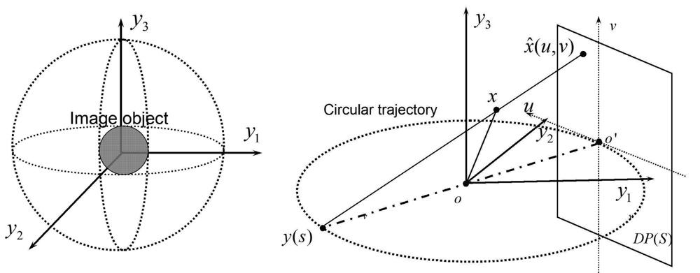
We propose the use of three independent, orthogonal to each other, circular isocentic scan-paths for X-ray projection acquisitions. Let a trajectory
C =
C1 ∪
C2 ∪
C3, as shown in
Figure 1.
Let
f(
x) is the density function to be constructed. Assume that the function is smooth and vanishes outside the ball:
where
r is the radius of the subject ball and R is the radius of the scanning circular. We assume that the physical detector is a planar-detector, which is denoted as
DP(
s), where s is the parameter of source point. Furthermore, let the planar-detector is at distance 2
R from the source, as shown in
Figure 1. Denote by (
u, v) the horizontal and vertical coordinates of the planar-detector plane, where
u is parallel to the tangent vector of source,
v is the normal vector of scanning trajectory and the origin is at the projection of the source point
y(
s) onto the detector plane.
Therefore, in the (
y1,
y2,
y3) coordinate system, any point on the detector plane can be characterized completely by use of (
u, v). It can be shown that:
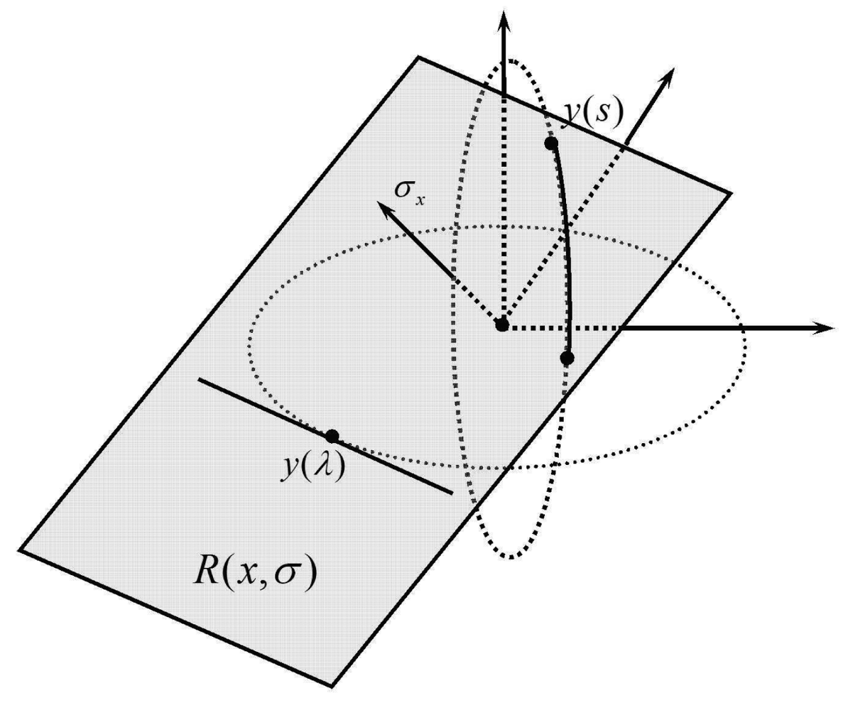
Figure 2 shows a filtering plane
R(x, σ) through the
y(s) and is tangent to other trajectory at point
y(λ). Without loss of generality we consider the source
y(s) ∈
C1 (the case
y(s) ∈
C2,3 is treated in a similar fashion). The point of tangency is given by either
y(λ) = (
R cosλ, 0,
R sinλ) or
y(λ) =(0,
R cosλ,
R sinλ). In the first case, the normal vector to the tangent plane is given by:
The equation of tangent plane, which is a filter plane, is given by:
Filtering lines on the detector are obtained by intersecting the detector plane and filtering planes. Substituting
Equation (20) and
Equation (23) into
Equation (24) and solving for
v, we obtain the equation of the filtering line on the planar-detector:
In the second case, the normal vector to the tangent plane is given by:
The equation of the filtering line on the planar-detector is given by:
4. Weighting Functions of Filtering Lines
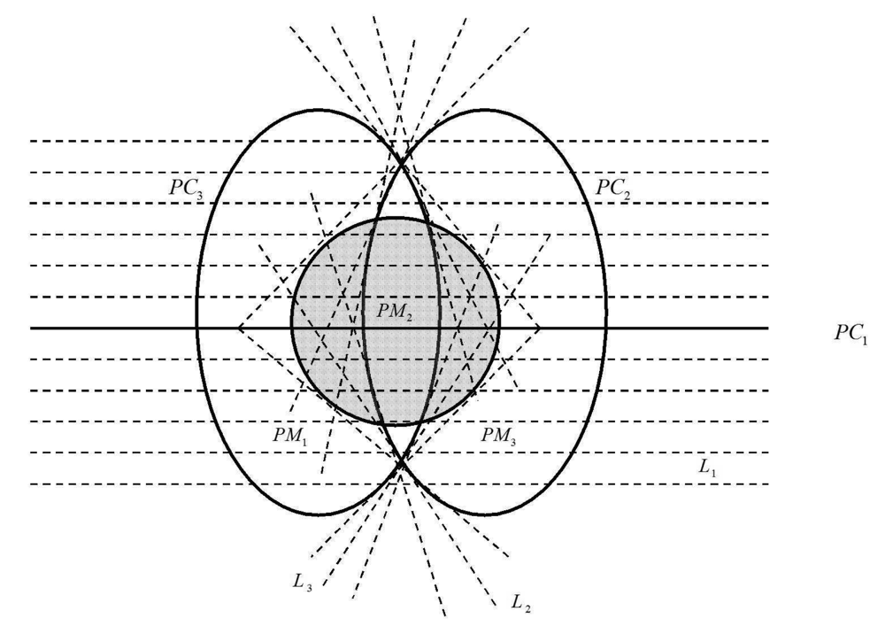
In the following, we define adequate filtering lines for the three-orthogonal scanning case. In order to define the different filtering lines, which are necessary to perform the three-orthogonal circular reconstruction, we first, introduce certain curves, which separate the planar-detector into different regions. As an example consider the X-ray source moving on the trajectory
C1. We project stereographically the trajectories
C2 and
C3 onto the detector plane as shown in
Figure 3. Let
PC2 and
PC3 denote these projections. The line
PC1 is the projection of trajectory
C1. Supp
f(
x) is supposed to be inside a ball centered as the origin and with sufficiently small radius
r <
R, so that the projection of ROI has a circular shape, as shown by the shaded region in
figure 3. The curves
PC2 and
PC3 split the entire ROI into three sub-ROIs:
PRm, m = 1,2,3. The object point x is projected into the area
PRm,m = 1,2,3. Let
x̂ denotes this projection.
If
x̂ ∈
PR1,
L(
φ) is the projection of the plane through
x with normal
σx(
s, φ). As
φ increase,
σx(
s, φ)
φ β⊥(
s, x) rotates in the clockwise direction on
DP(
s). From definition of
kx(
s, φ) with
equation (14) k is discontinuous if
L(
φ) is parallel to
y'(
s) or is tangent to
C2. In the first case, such a plane has six points of intersection with
C =
C1 ∪
C2 ∪
C3, so
k = 1/6 on the side of the jump, where
y'(
s) ·
σ > 0 and
k = −1/6 on the other side. The filtering line is parallel to
y'(
s), which is denoted as
L1(see the dot-dashed lines in
Figure 3). The corresponding weighting function of filtering line
L 1 is
wx(
s, φ1) = 1/3. In the second case, the number of intersection changes form four to six. So the filtering line is tangent to
C2, which is denoted as
L2 (see the dot-dashed lines in
Figure 3). For the signum function in
Equation (14) is unchagened, the corresponding weighting function of filtering line
L2 is
wx(
s, φ2) = 1/12. If
x̂ ∈
PR2,
k is discontinuous only
L(
φ) is parallel to
y'(
s). So the filtering line
L1 is parallel to
y(
s). The corresponding weight function is
wx(
s, φ1) = 1/3. If
x̂ ∈
PR3,
k is discontinuous if
L(
φ) is parallel to
y'(
s) or is tangent to
C3. In the first case, such a plane has six points of intersection with trajectory, so
k = 1/6 on the side of the jump, where
y'(
s) ·
e > 0 and
k = −1/6 on the other side. The filter line is parallel to
y'(
s), which is denoted as
L1 (as shown in
Figure 3).The corresponding weighting function of filtering line
L1 is
wx(
s, φ1) = 1/3. In the second case, the number of intersection changes form four to six. So the filtering line is tangent to
C3, which is denoted as
L3(see the dot-dashed lines in
Figure 3). The corresponding weighting function of filtering line
L3 is
wx(
s, φ3) = 1/12.
Figure 3 summarizes the above information.

 2 to ℝ3 × ℝ3 as: