Spatial Forecast of Landslides in Three Gorges Based On Spatial Data Mining

Abstract
:1. Introduction
2. Choice of Forecast Factors
2.1. Spectral Factors
2.2. Textural Factors
- Contrast
- Correlation
- Mean
- Entropy
- Homogeneity
- Dissimilarity
- Angle Second Moment
- Variancein which p(i, j) is the pixel value in the position (i, j) in GLCM.
2.3. Vegetation Coverage Factors
2.4. Geological, Physiognomy and Environmental Factors
3. Decision Tree C4.5 Algorithm
3.1. Production of Decision Tree
3.2. Pruning of Decision Tree
4. Experiments of Criterion Mining and Spatial Intelligent Forecast of Landslides in Three Gorges
5. Conclusions
Acknowledgments
References and Notes
- Kumar, K.V.; Lakhera, R.C.; Martha, T.R.; Chatterjee, R.S.; Bhattacharya, A. Analysis of the 2003 Varunawat Landslide, Uttarkashi, India using Earth Observation data. Environ. Geol 2008, 55, 789–799. [Google Scholar]
- Borgatti, L.; Corsini, A.; Marcato, G.; Ronchetti, F.; Zabuski, L. Appraise the structural mitigation of landslide risk via numerical modelling: a case study from the northern apennines. Georisk 2008, 2, 141–160. [Google Scholar]
- Nandi, A.; Shakoor, A. Application of logistic regression model for slope instability prediction in Cuyahoga River Watershed, Ohio, USA. Georisk 2008, 2, 16–27. [Google Scholar]
- Kumar, S.V.; Bhagavanulu, D.V.S. Effect of Deforestation on Landslides in Nilgiris District. J. Indian Soc. Remote Sens 2008, 36, 105–108. [Google Scholar]
- Yin, K.L.; Yan, T.Z. Landslide Forecast and Related Models. Chin. J. Rock Mech. Eng 1996, 15, 1–8. [Google Scholar]
- Yin, K.L. Mechanism and dynamic simulation of Landslide by precipitation. Geol. Sci. Tech. Info 2002, 22, 75–78. [Google Scholar]
- Yan, T.Z.; Yin, K.L. Landslide. Proceedings of Hydrological and Engineering Geology, Beijing, China, June 1992; pp. 155–160.
- Xie, J.M.; Liu, L.L.; Yin, K.L. Warning system for rain-induced Landslides based on internet in Zhejiang Province, China. Geol. Sci. Tech. Info 2003, 22, 101–105. [Google Scholar]
- Zhu, L.F.; Wu, X.C. Risk Zonation of Landslide in China based on Information Content Model. J. Earth Sci. Environ 2004, 26, 52–56. [Google Scholar]
- Shan, X.J.; Ye, H.; Li, Z.F. Prediction of regional Landslide danger areas using AI-GIS based on environment factors: an example of Lantau Island. Hongkong Geol. Sci. Tech. Info 2004, 23, 109–112. [Google Scholar]
- Lumb, P. Slope failures in Hong Kong. Quart. J. Eng. Geol 1975, 8, 31–65. [Google Scholar]
- Ruxton, B.P. Slope problems in Hong Kong, a geological appraisal. H. K. Eng 1980, 8, 31–39. [Google Scholar]
- Fourie, A.B.; Anderson, M.G.; Hartshorne, J.; Lloyd, D.M.; Othman, A. Predicting rainfall-induced slope instability. Proc. Inst. Civ. Eng. – Geotech. Eng 1996, 119, 211–218. [Google Scholar]
- Collison, A.J.C.; Anderson, M.G. Using a combined slope hydrology-stability model to identify suitable conditions for landslide prevention by vegetation in the humid tropics. Earth Surf. Proc. Land 1996, 21, 737–747. [Google Scholar]
- Evans, N.C. Natural terrain landslide study: preliminary assessment of the influence of rainfall on natural terrain landslide initiation. H. K. Geotech. Eng. Off 1997, 28–29. [Google Scholar]
- Carrara, A.; Cardinali, M.; Detti, R.; Guzzetti, F.; Pasqui, V.; Reichenbach, P. GIS Techniques and Statistical Models in Evaluating Landslide Hazard. Earth Surf. Proc. Land 1991, 16, 427–445. [Google Scholar]
- Brabb, E.E. Innovative approach to landslide hazard mapping. Proceedings of 4th International Symposium on Landslides, Toronto, Canada, July 1984; pp. 307–324.
- Zai, X.Y.; Xue, H.F.; Lei, X.W. The Remote Sensing Image Classification Research Based on Mining Classification Rules on the Spatial Database. J. Remote Sens 2006, 10, 332–338. [Google Scholar]
- Sun, Q.X.; Fang, T.; Guo, D.Z. Zonging effect in spatial data mining and its application in coal mine. J. Chn. Coal Soc 2007, 32, 804–807. [Google Scholar]
- Chen, X.Y. The Classification of Remote Sensing Image Based on Spatial Data Mining and Knowledge Discovery; Fujian Normal University Press: Fuzhou, China, 2007. [Google Scholar]
- Lin, Y.B.; Lin, Y.P.; Deng, D.P.; Chen, K.W. Integrating remote sensing data with directional two-dimensional wavelet analysis and open geospatial techniques for efficient disaster monitoring and management. Sensors 2008, 8, 1070–1089. [Google Scholar]
- Delacourt, C.; Raucoules, D.; Mouélic, S.L.; Carnec, C.; Feurer, D.; Allemand, P.; Cruchet, M. Observation of a large Landslide on La Reunion Island using differential Sar Interferometry (JERS and Radarsat) and correlation of optical (Spot5 and Aerial) images. Sensors 2009, 9, 616–630. [Google Scholar]
- Zhao, J.H.; Chen, H.L.; Yang, S.F. Landslide risk assessment based on decision tree arithmetic. J. Zhejiang Univ 2004, 31, 465–470. [Google Scholar]
- Ma, Z.J.; Chen, H.L.; Yang, S.F. Prediction of landslide hazard based on support vector machine theory. J. Zhejiang Univ 2003, 30, 592–596. [Google Scholar]
- Pandey, A.; Dabral, P.P.; Chowdary, V.M.; Yadav, N.K. Landslide hazard Zonation using remote sensing and GIS: a case study of Dikrong River Basin, Arunachal Pradesh. Indian Environ. Geol 2008, 54, 1517–1529. [Google Scholar]
- Zhang, W.J.; Wang, W.H. Landslide Occurring Probability Decision Based on Remote Sensing and Quantification Theory II. In In International Archives of the Photogrammetry, Remote Sensing and Spatial Information Sciences; Beijing, China, 2008; Volume XXXVII, Part B 8,; pp. 925–928. [Google Scholar]
- Hua, L.Z.; Cui, S.H.; Li, X.H.; Yin, K.; Qiu, Q.Y. Remote sensing identification of earthquake trigged landslides and their impacts on ecosystem services: a case study of Wenchuan county. Acta Ecol. Sinica 2008, 28, 5909–5916. [Google Scholar]
- Park, N.W.; Chi, K.H. Quantitative assessment of landslide susceptibility using high-resolution remote sensing data and a generalized additive model. Int. J. Remote Sens 2009, 29, 247–264. [Google Scholar]
- Hunt, G.R. Spectroscopic Properties of Rocks and Minerals. In Handbook of Physical Properties of Rocks; CRC Press: Boca Raton, FL, USA, 1982; Volume I, pp. 128–188. [Google Scholar]
- Kruse, F.A.; Lefkoff, A.B.; Boardman, J.W.; Heidebrecht, K.B.; Shapiro, A.T.; Barloon, P.J.; Goetz, A.F.H. The spectral Image Processing System (SIPS) interactive visualization and analysis of imaging spectrometer data. Remote Sens. Environ 1993, 44, 145–163. [Google Scholar]
- Gani, N.D.; Abdelsalam, M.G. Remote sensing analysis of the Gorge of the Nile, Ethiopia with emphasis on Dejen-Gohatsion region. J. Afr. Earth Sci 2006, 44, 135–150. [Google Scholar]
- Lawrence, C.R.; Colin, J.S.; John, C.M. Hyperspectral analysis of the ultramafic complex and adjacent lithologies at MordNT. Austrlia. Remote Sens. Environ 2004, 91, 419–431. [Google Scholar]


| engineering rock group = 0.0000: dangerous (3.0/1.1) |
| engineering rock group = 1.6000: unstable (26.0/1.3) |
| engineering rock group = 1.2000: |
| | slope structure = 0.0000: basically stable (0.0) |
| | slope structure = 0.9000: basically stable (66.0/1.4) |
| | slope structure = 1.2000: basically stable (0.0) |
| | slope structure = 0.6000: |
| | | band3dissimilarity <= 4.2222 : |
| | | | band3variance <= 11.8765 : basically stable (340.0/3.9) |
| | | | band3variance > 11.8765 : |
| | | | | water level of reservoir = 0.1000: stable (9.0/2.4) |
| | | | | water level of reservoir = 0.2000: basically stable (2.0/1.0) |
| | | | | water level of reservoir = 0.4000: stable (0.0) |
| | | | | water level of reservoir = 0.5000: basically stable (2.0/1.0) |
| | | | | water level of reservoir = 0.0000: stable (0.0) |
| | | band3dissimilarity > 4.2222 : |
| | | | water level of reservoir = 0.1000: stable (52.0/1.4) |
| | | | water level of reservoir = 0.2000: basically stable (7.0/1.3) |
| | | | water level of reservoir = 0.4000: basically stable (2.0/1.0) |
| | | | water level of reservoir = 0.5000: basically stable (1.0/0.8) |
| | | | water level of reservoir = 0.0000: stable (0.0) |
| | slope structure = 1.5000: |
| | | band2 <= 77 : basically stable (36.0/1.4) |
| | | band2 > 77 : |
| | | | water level of reservoir = 0.4000: unstable (23.0/1.3) |
| | | | water level of reservoir = 0.5000: unstable (0.0) |
| | | | water level of reservoir = 0.0000: unstable (0.0) |
| | | | water level of reservoir = 0.1000: |
| | | | | dem > 139 : unstable (15.0/1.3) |
| | | | | dem <= 139 : |
| | | | | | dem <= 41 : unstable (2.0/1.0) |
| | | | | | dem > 41 : basically stable (59.0/1.4) |
| | | | water level of reservoir = 0.2000: |
| | | | | band4 <= 150 : |
| | | | | | band3variance <= 8.1728 : unstable (387.0/1.4) |
| | | | | | band3variance > 8.1728 : |
| | | | | | | dem <= 78 : basically stable (4.0/1.2) |
| | | | | | | dem > 78 : unstable (50.0/2.6) |
| | | | | band4 > 150 : |
| | | | | | dem <= 126 : basically stable (4.0/1.2) |
| | | | | | dem > 126 : unstable (10.0/1.3) |
| | slope structure = 0.3000: |
| | | NDVI <= 0.2917 : unstable (38.0/1.4) |
| | | NDVI > 0.2917 : |
| | | | band4 <= 158 : |
| | | | | band3 <= 37 : |
| | | | | | dem <= 337 : stable (13.0/1.3) |
| | | | | | dem > 337 : basically stable (18.0/1.3) |
| | | | | band3 > 37 : |
| | | | | | aspect <= 298.811 : |
| | | | | | | band4 <= 155 : basically stable (90.0/1.4) |
| | | | | | | band4 > 155 : |
| | | | | | | | slope <= 39.0801 : basically stable (18.0/1.3) |
| | | | | | | | slope > 39.0801 : stable (2.0/1.0) |
| | | | | | aspect > 298.811 : |
| | | | | | | band4 <= 151 : basically stable (7.0/1.3) |
| | | | | | | band4 > 151 : unstable (3.0/1.1) |
| | | | band4 > 158 : |
| | | | | slope > 10.1868 : stable (71.0/1.4) |
| | | | | slope <= 10.1868 : |
| | | | | | aspect <= 276.87 : basically stable (6.0/1.2) |
| | | | | | aspect > 276.87 : unstable (2.0/1.8) |
| engineering rock group = 2.0000: |
| | slope structure = 0.6000: dangerous (22.0/1.3) |
| | slope structure = 0.0000: unstable (0.0) |
| | slope structure = 0.3000: unstable (305.0/1.4) |
| | slope structure = 0.9000: dangerous (39.0/1.4) |
| | slope structure = 1.2000: dangerous (11.0/1.3) |
| | slope structure = 1.5000: |
| | | dem > 362 : unstable (25.0/1.3) |
| | | dem <= 362 : |
| | | | aspect <= 259.38 : |
| | | | | dem <= 147 : dangerous (53.0/1.4) |
| | | | | dem > 147 : |
| | | | | | band3 <= 46 : dangerous (19.0/2.5) |
| | | | | | band3 > 46 : |
| | | | | | | aspect <= 197.526 : |
| | | | | | | | band3homogeneity > 0.5222 : dangerous (19.0/1.3) |
| | | | | | | | band3homogeneity <= 0.5222 : |
| | | | | | | | | band3correlation > −3.0981 : unstable (9.0/1.3) |
| | | | | | | | | band3correlation <= −3.0981 : |
| | | | | | | | | | dem <= 161 : unstable (6.0/1.2) |
| | | | | | | | | | dem > 161 : |
| | | | | | | | | | | band4 > 145 : unstable (6.0/1.2) |
| | | | | | | | | | | band4 <= 145 : |
| | | | | | | | | | | | band3mean <= 19.6667 : dangerous (44.0/7.2) |
| | | | | | | | | | | | band3mean > 19.6667 :[S1] |
| | | | | | | aspect > 197.526 : |
| | | | | | | | band4 > 128 : unstable (58.0/2.6) |
| | | | | | | | band4 <= 128 : |
| | | | | | | | | water level of reservoir = 0.1000: unstable (1.0/0.8) |
| | | | | | | | | water level of reservoir = 0.4000: dangerous (4.0/1.2) |
| | | | | | | | | water level of reservoir = 0.5000: unstable (0.0) |
| | | | | | | | | water level of reservoir = 0.0000: unstable (0.0) |
| | | | | | | | | water level of reservoir = 0.2000: |
| | | | | | | | | | band3mean <= 20.7778 : |
| | | | | | | | | | | dem <= 187 : unstable (4.0/1.2) |
| | | | | | | | | | | dem > 187 : dangerous (8.0/1.3) |
| | | | | | | | | | band3mean > 20.7778 : |
| | | | | | | | | | | band4 > 118 : unstable (18.0/1.3) |
| | | | | | | | | | | band4 <= 118 : |
| | | | | | | | | | | | band3mean <= 23.6667 : dangerous (7.0/1.3) |
| | | | | | | | | | | | band3mean > 23.6667 : unstable (2.0/1.0) |
| | | | aspect > 259.38 : |
| | | | | band4 <= 152 : dangerous (195.0/7.3) |
| | | | | band4 > 152 : |
| | | | | | band3entropy <= 2.0432 : dangerous (2.0/1.0) |
| | | | | | band3entropy > 2.0432 : unstable (5.0/1.2) |
| engineering rock group = 0.4000: |
| | slope structure = 0.6000: basically stable (0.0) |
| | slope structure = 0.0000: basically stable (0.0) |
| | slope structure = 0.3000: unstable (14.0/1.3) |
| | slope structure = 0.9000: basically stable (0.0) |
| | slope structure = 1.2000: basically stable (0.0) |
| | slope structure = 1.5000: |
| | | dem <= 263 : basically stable (231.0/1.4) |
| | | dem > 263 : |
| | | | band3variance > 1.284 : stable (73.0/1.4) |
| | | | band3variance <= 1.284 : |
| | | | | aspect <= 257.735 : |
| | | | | | slope <= 3.7242 : |
| | | | | | | band3secondmoment <= 0.1852 : stable (8.0/1.3) |
| | | | | | | band3secondmoment > 0.1852 : basically stable (3.0/2.1) |
| | | | | | slope > 3.7242 : |
| | | | | | | band4 <= 128 : stable (2.0/1.0) |
| | | | | | | band4 > 128 : basically stable (68.0/3.8) |
| | | | | aspect > 257.735 : |
| | | | | | 3/2 <= 0.4949 : basically stable (3.0/2.1) |
| | | | | | 3/2 > 0.4949 : stable (29.0/1.4) |
| Subtree [S1] |
| band3contrast > 19.2222 : dangerous (6.0/1.2) |
| band3contrast <= 19.2222 : |
| | band3homogeneity <= 0.3951 : unstable (16.0/2.5) |
| | band3homogeneity > 0.3951 : |
| | | band3contrast <= 3.8889 : unstable (7.0/2.4) |
| | | band3contrast > 3.8889 : dangerous (6.0/1.2) |
| Forecast criterions of stable region: |
| Rule 1: band3variance > 1.284 & engineering rock group = 0.4000 & dem > 263 -> class stable [98.1%] |
| Rule 2: band4 > 158 & slope > 10.1868 & engineering rock group = 1.2000 & slope structure = 0.3000 -> class stable [98.1%] |
| Rule 3: 3/2 > 0.4949 & engineering rock group = 0.4000 & aspect > 257.735 & dem > 263 -> class stable [98.0%] |
| Rule 4: water level of reservoir = 0.1000 & band3dissimilarity > 4.2222 & slope structure = 0.6000 -> class stable [97.4%] |
| Rule 5: band1 > 62 & dem <= 75 & water level of reservoir = 0.1000 & slope structure = 0.6000 -> class stable [97.0%] |
| Rule 6: band4 > 155 & slope > 39.0801 & engineering rock group = 1.2000 & slope structure = 0.3000 -> class stable [97.0%] |
| Rule 7: band3secondmoment <= 0.1852 & engineering rock group = 0.4000 & slope <= 3.7242 & dem > 263 - > class stable [95.2%] |
| Rule 8: water level of reservoir = 0.1000 & band3variance > 11.8765 & slope structure = 0.6000 -> class stable [94.6%] |
| Rule 9: band3 <= 37 & dem <= 337 & slope structure = 0.3000 -> class stable [92.2%] |
| Rule10: band4 <= 128 & engineering rock group = 0.4000 & dem > 263 -> class stable [89.1%] |
| Rule 11: band3variance <= 11.8765 & dem > 75 & engineering rock group = 1.2000 & slope structure = 0.6000 -> class basically stable [99.5%] |
| Forecast criterions of basically stable region: |
| Rule1: dem <= 263 & engineering rock group = 0.4000 & slope structure = 1.5000 -> class basically stable [99.4%] |
| Rule2: band3variance <= 11.8765 & band3dissimilarity <= 4.2222 & band1 <= 62 & slope structure = 0.6000 -> class basically stable [99.4%] |
| Rule 3: water level of reservoir = 0.2000 & slope structure = 0.6000 -> class basically stable [99.3%] |
| Rule 4: NDVI > 0.2917 & band3 > 37 & band4 <= 155 & engineering rock group = 1.2000 & aspect <= 298.811 & slope structure = 0.3000 -> class basically stable [98.5%] |
| Rule 5: dem > 41 & dem <= 139 & water level of reservoir = 0.1000 & slope structure = 1.5000 -> class basically stable [98.4%] |
| Rule 6: NDVI > 0.2917 & band3 > 37 & slope <= 39.0801 & engineering rock group = 1.2000 & band4 <= 158 & slope structure = 0.3000 & aspect <= 298.811 -> class basically stable [98.0%] |
| Rule 7: engineering rock group = 1.2000 & slope structure = 0.9000 -> class basically stable [97.9%] |
| Rule 8: dem > 337 & engineering rock group = 1.2000 & slope structure = 0.3000 -> class basically stable [97.8%] |
| Rule 9: NDVI > 0.2917 & band3 > 37 & band4 <= 151 & engineering rock group = 1.2000 & slope structure = 0.3000 -> class basically stable [97.6%] |
| Rule 10: band2 <= 77 & engineering rock group = 1.2000 & slope structure = 1.5000 -> class basically stable [96.2%] |
| Rule 11: band3variance <= 1.284 & band4 > 128 & slope > 3.7242 & aspect <= 257.735 & engineering rock group = 0.4000 -> class basically stable [95.9%] |
| Rule 12: 3/2 <= 0.4949 & band3variance <= 1.284 -> class basically stable [93.2%] |
| Rule 13: band3variance > 8.1728 & dem <= 78 & engineering rock group = 1.2000 & slope structure = 1.5000 -> class basically stable [90.6%] |
| Rule 14: band4 > 150 & dem <= 126 & engineering rock group = 1.2000 & slope structure = 1.5000 -> class basically stable [89.1%] |
| Rule 15: engineering rock group = 1.2000 & water level of reservoir = 0.5000 & slope structure = 0.6000 -> class basically stable [87.1%] |
| Forecast criterions of unstable region: |
| Rule 1: engineering rock group = 2.0000 & slope structure = 0.3000 -> class unstable [99.5%] |
| Rule 2: NDVI <= 0.2917 & slope structure = 0.3000 -> class unstable [99.4%] |
| Rule 3: dem > 139 & engineering rock group = 1.2000 & slope structure = 1.5000 -> class unstable [99.3%] |
| Rule 4: dem > 78 & engineering rock group = 1.2000 & water level of reservoir = 0.2000 & slope structure = 1.5000 -> class unstable [99.2%] |
| Rule 5: dem <= 41 & engineering rock group = 1.2000 & slope structure = 1.5000 -> class unstable [98.8%] |
| Rule 6: dem > 362 & slope structure = 1.5000 -> class unstable [98.4%] |
| Rule 7: band3mean <= 20.7778 & band3 > 46 & dem <= 187 & slope structure = 1.5000 & aspect <= 259.38 & dem > 147 -> class unstable [97.8%] |
| Rule 8: band3 > 46 & band4 > 128 & slope structure = 1.5000 & aspect > 197.526 & aspect <= 259.38 & dem > 147 -> class unstable [97.1%] |
| Rule 9: band3mean > 19.6667 & band3homogeneity <= 0.3951 & band3contrast <= 19.2222 & dem <= 362 & engineering rock group = 2.0000 & aspect <= 197.526 & dem > 147 -> class unstable [96.5%] |
| Rule10: band3 > 46 & band4 > 145 & slope structure = 1.5000 & aspect <= 259.38 & dem > 147 -> class unstable [96.3%] |
| Rule11: band3homogeneity <= 0.5222 & band3correlation > −3.0981 & engineering rock group = 2.0000 & band3 > 46 & aspect <= 259.38 & dem > 147 & dem <= 362 -> class unstable [96.2%] |
| Rule 12: engineering rock group = 1.6000 -> class unstable [94.8%] |
| Rule13: band3mean > 20.7778 & band4 > 116 & water level of reservoir = 0.2000 & slope structure = 1.5000 & aspect > 197.526 & aspect <= 259.38 & dem > 147 -> class unstable [93.8%] |
| Rule 14: band3mean > 19.6667 & band3homogeneity <= 0.5222 & band3contrast <= 3.8889 & band4 <= 145 & aspect <= 197.526 & dem > 147 & dem <= 362 -> class unstable [93.7%] |
| Rule 15: band4 > 151 & band4 <= 158 & aspect > 298.811 & slope structure = 0.3000 -> class unstable [93.6%] |
| Rule 16: water level of reservoir = 0.4000 & band3mean <= 19.6667 & slope structure = 1.5000 & aspect <= 259.38 -> class unstable [93.6%] |
| Rule17: engineering rock group = 0.4000 & slope structure = 0.3000 -> class unstable [90.6%] |
| Rule 18: band3mean > 20.7778 & band3homogeneity > 0.304 & water level of reservoir = 0.2000 & slope structure = 1.5000 & band1 > 65 & aspect > 259.38 -> class unstable [87.9%] |
| Rule 19: water level of reservoir = 0.1000 & engineering rock group = 2.0000 & band4 <= 128 -> class unstable [82.0%] |
| Rule20: band3entropy > 2.0432 & engineering rock group = 2.0000 & slope structure = 1.5000 & band4 > 152 & aspect > 259.38 -> class unstable [75.8%] |
| Forecast criterions of dangerous region: |
| Rule 1: dem <= 147 & engineering rock group = 2.0000 & slope structure = 1.5000 -> class dangerous [97.9%] |
| Rule 2: engineering rock group = 2.0000 & slope structure = 0.9000 -> class dangerous [96.5%] |
| Rule 3: band4 <= 152 & engineering rock group = 2.0000 & slope structure = 1.5000 & aspect > 259.38 & dem <= 362 -> class dangerous [96.2%] |
| Rule 4: water level of reservoir = 0.4000 & engineering rock group = 2.0000 & slope structure = 1.5000 & band4 <= 128 -> class dangerous [95.0%] |
| Rule 5: band3mean <= 20.7778 & dem > 187 & engineering rock group = 2.0000 & band4 <= 128 -> class dangerous [94.8%] |
| Rule 6: band3homogeneity > 0.5222 & engineering rock group = 2.0000 & slope structure = 1.5000 & aspect <= 197.526 -> class dangerous [94.8%] |
| Rule 7: band3 <= 46 & engineering rock group = 2.0000 & aspect <= 259.38 & dem <= 362 -> class dangerous [94.4%] |
| Rule 8: engineering rock group = 2.0000 & slope structure = 0.6000 -> class dangerous [93.9%] |
| Rule 9: band3mean > 19.6667 & band3contrast > 19.2222 & engineering rock group = 2.0000 & slope structure = 1.5000 & dem <= 362 -> class dangerous [93.2%] |
| Rule10: band3mean <= 23.6667 & engineering rock group = 2.0000 & band4 <= 118 & aspect > 197.526 -> class dangerous [88.5%] |
| Rule 11: slope structure = 1.2000 -> class dangerous [88.2%] |
| Rule 12: band3mean <= 19.6667 & engineering rock group = 2.0000 & band3correlation <= −3.0981 & band4 <= 145 & aspect <= 197.526 & dem > 161 & dem <= 362 -> class dangerous [87.9%] |
| Rule 13: band3homogeneity > 0.3951 & band3contrast > 3.8889 & engineering rock group = 2.0000 & slope structure =1.5000 & band3correlation <= −3.0981 & aspect <= 197.526 & dem > 161 & dem <= 362 -> class dangerous [87.1%] |
| Rule 14: engineering rock group = 0.0000 -> class dangerous [63.0%] |
| Default Class: basically stable |
| Values of forecast indexes | Connotation |
|---|---|
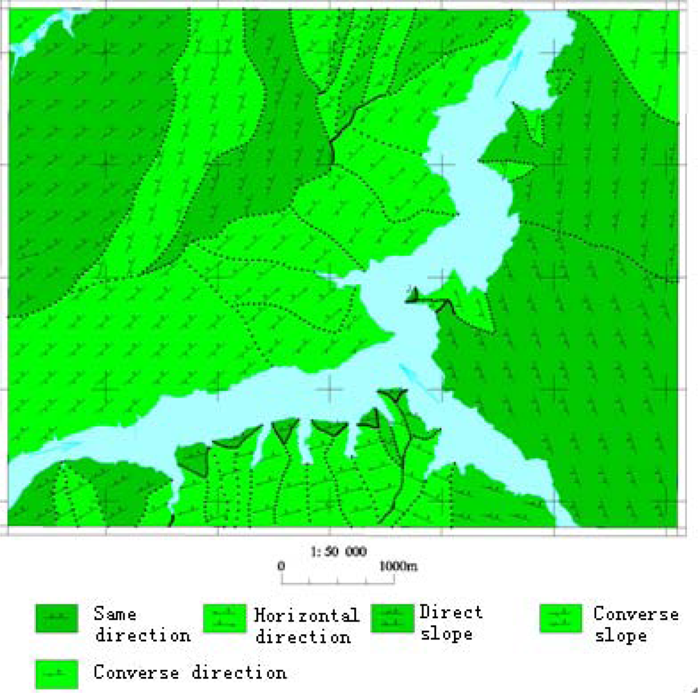
| slope structure=1.5 | Slopes with the same direction |
| slope structure=0.6 | Slopes with the converse direction |
| slope structure=0.3 | Slopes with the horizontal direction |
| slope structure=0.9 | Converse slope |
| slope structure=1.2 | Direct slope |
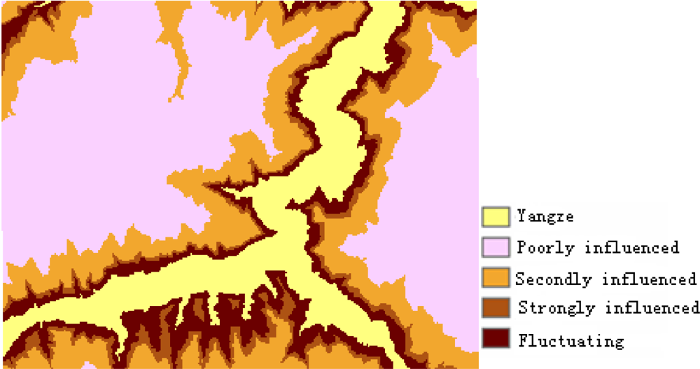
| water level of reservoir=0.1 | Poorly influenced region |
| water level of reservoir=0.2 | Medium influenced region |
| water level of reservoir=0.4 | Strongly influenced region |
| water level of reservoir=0.5 | Fluctuating region |
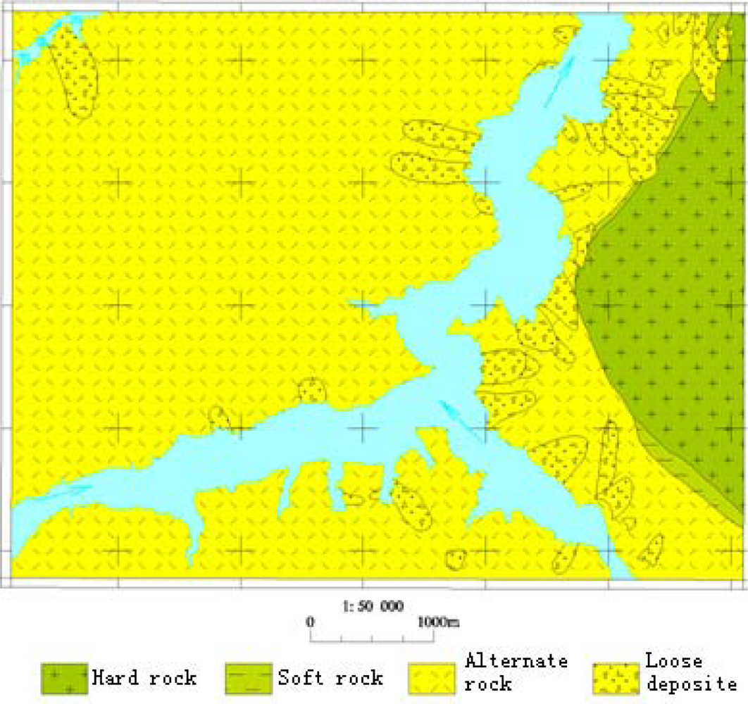
| engineering rock group=1.2 | Alternate soft and hard stratum |
| engineering rock group=1.6 | Hard rock |
| engineering rock group=0.4 | Soft rock |
| engineering rock group=2 | Loose deposits |
| Precision assessment | Unsupervised method | Supervised method | Decision tree | ||||
|---|---|---|---|---|---|---|---|
| IsoData Method | K-Means Method | Paralle-lepiped | Minimum Distance | Mahalanobis Distance | Maximum likelihood | ||
| Overall Accuracy | 15.99% | 15.99% | 46.59% | 28.21% | 73.44% | 80.97 % | 99.15% |
| Kappa Coefficient | 0 | 0 | 0.2126 | 0.0960 | 0.6311 | 0.7322 | 0.9876 |
© 2009 by the authors; licensee MDPI, Basel, Switzerland This article is an open-access article distributed under the terms and conditions of the Creative Commons Attribution license (http://creativecommons.org/licenses/by/3.0/).
Share and Cite
Wang, X.; Niu, R. Spatial Forecast of Landslides in Three Gorges Based On Spatial Data Mining. Sensors 2009, 9, 2035-2061. https://doi.org/10.3390/s90302035
Wang X, Niu R. Spatial Forecast of Landslides in Three Gorges Based On Spatial Data Mining. Sensors. 2009; 9(3):2035-2061. https://doi.org/10.3390/s90302035
Chicago/Turabian StyleWang, Xianmin, and Ruiqing Niu. 2009. "Spatial Forecast of Landslides in Three Gorges Based On Spatial Data Mining" Sensors 9, no. 3: 2035-2061. https://doi.org/10.3390/s90302035