Acoustic Sensor Planning for Gunshot Location in National Parks: A Pareto Front Approach


Abstract
:
1. Introduction
2. Gunshot Location
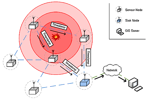
2.1. System architecture
- Sensor nodes: The sensor nodes in known positions are equipped with the necessary hardware for the detection of acoustic events. They can discriminate between normal and shot segment classes in audio streams. When a sensor node detects a sound event, it transmits a packet with information about the type of sound event and a sound timestamp to a special node, the sink.
- Sink nodes: Sink nodes collect the packets sent by sensor nodes and deliver them to the GIS server to calculate the position of the sound event. Sink nodes may be sensing nodes as well.
- GIS server: Using the information from the sink nodes, the GIS server estimates the position of the acoustic event by means of a hyperbolic method, described in Section 2.2.
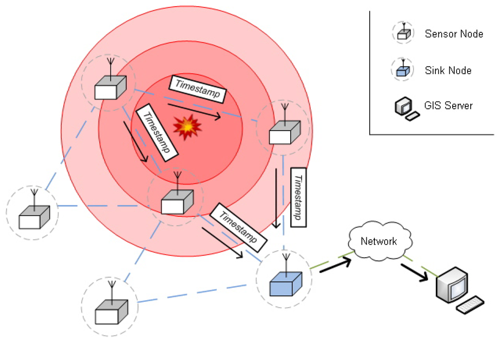
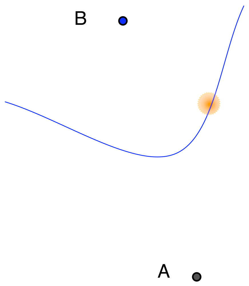
2.2. Source location procedure
- The speed of sound varies depending on altitude, humidity and air temperature. As we have mentioned, multi-path propagation affects the accuracy of acoustic signal detection. Single spread-spectrum techniques such as those in [27] largely mitigate it.
- The microphone directionality or polar pattern affects the result.
- The clock drift may drastically vary in time due to environmental temperature and humidity changes. In Section 2.3. we propose an approach to reduce sensor clock deviations.
2.3. Synchronization schema
- Level discovery: This step is similar to the level discovery stage in TPSN [19]. Before the synchronization process takes place, the network has to organize itself as a hierarchical tree, beginning at a root node (in our case we choose the sink). According to the minimum number of hops to the sink, a level is assigned to each node (level 0 to the root). To compute the tree, the process starts at the root, broadcasting a level discovery packet to the nodes at level 0. The nodes that receive this packet are marked as children of the root node, and they set their level to 1. The nodes ignore further level discovery packets with greater or equal level numbers. Then, level 1 nodes broadcast their level discovery packets, and so on. Note that this process also permits discover of optimal communication paths (in number of hops) to the root, and, thus, it is valid for network routing.
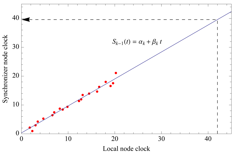
- Synchronization: Once the hierarchical network structure is completed, the synchronization process may start. In general, level k nodes synchronize their children (of level k + 1).Besides its own local clock, a sensor node will maintain an estimation of its synchronizer node clock in the upper hierarchical level. The approximation consists of calculating the regression line of those two clocks. Previously, the level k node receives several synchronized time-stamps of level k – 1 (see Figure 4), which are broadcast following the tree structure that was created at the level discovery step. Figure 4 shows the regression line used to calculate the parent node clock in a level k node. Value αk represents the clock offset at reference time t = 0, and the slope βk is the rate of change (clock drift) of the local clock.Once a node detects a gunshot, it sends the event to its parent node in the upper level, according to the parent time clock. After one or more hops, level 0 (sink node) will receive estimations of the detection time that are synchronized with the sink clock, from one or more level 1 nodes. This way, local clock exchanges do not spend power. Since clock drift varies slowly, the regression line must only be calculated every 6 or 8 hours, according to our tests with MicaZ motes. Only large temperature variations affect the regression line slope, requiring node re-synchronization.
3. Optimization Model
- ω1(s, x) corresponds to propagation distance through wood space.
- ω2(s, x) corresponds to propagation distance through open space.
Remark 1
4. Solving the Optimization Model
4.1. Alternative approaches
4.2. Derivative-free unconstrained minimization
- A1. f(S) : IR2p → IR is bounded below, and remains in a compact set,
- A2. f(S) has directional derivatives f′(S, D) everywhere defined:
- A3. The unit directions D1, …, Dn positively span R2p.
- A4. The function ν(·) : IR+ → IR+ is little-o of τ, that is: lim ν(τ)/τ = 0
- A5. The reference values are upper bounds of f(·), i.e., φi ≥ f(Si) for all i, and decrease sufficiently after a given finite number of successful iterations.
- A6. f(S) is strictly differentiable or locally convex at all limit points of the sequence generated by the algorithm.
Remark 2
Remark 3
Remark 4
Remark 5
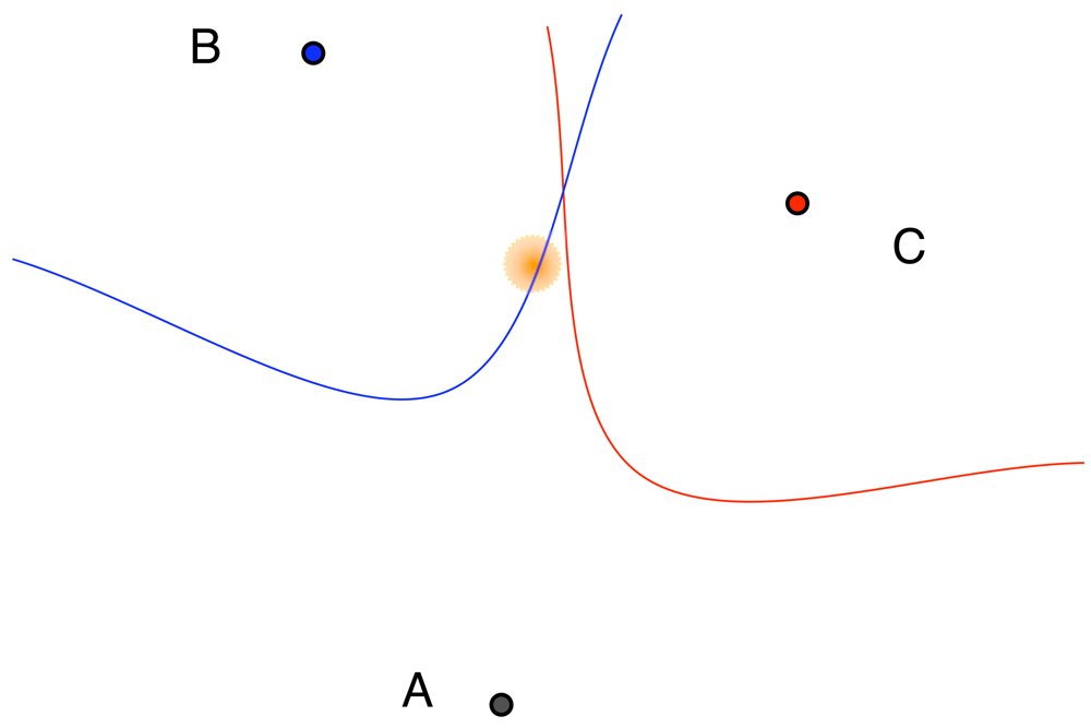
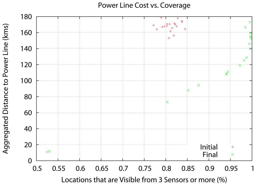
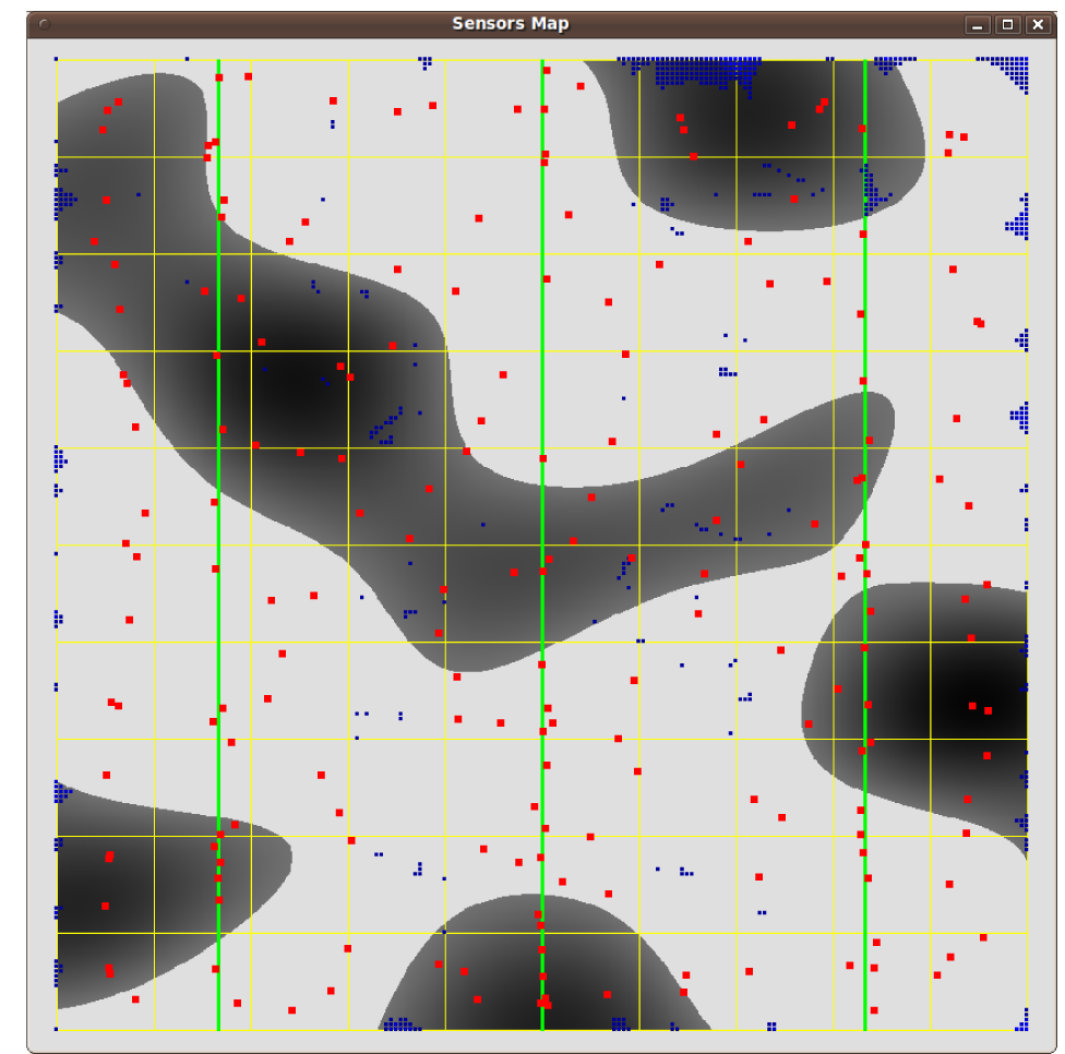
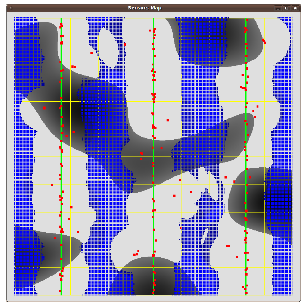
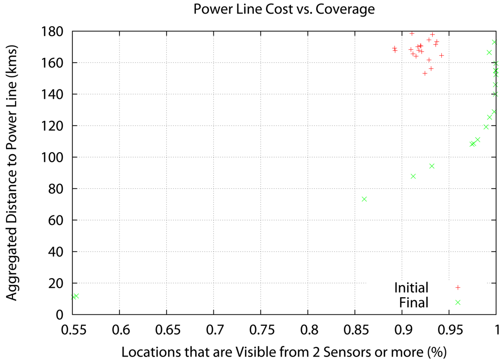
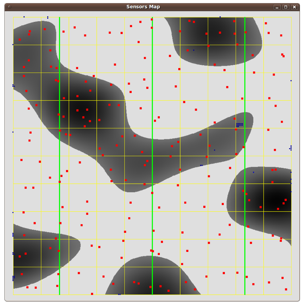
5. Numerical Tests
- Δ = 0.1 Km, i.e., the method stops when the maximum sensor displacement is under 100 m.
- ετ = 1
- τ = 5
- max_success= 40 (20%p), but we do not allow τ > 8.
- We initially set φ to the value of the objective function at the starting point.
- α = 0, i.e., we perform a monotone derivative-free search.
- Finally, we set ν(τΔ) = 0.001(τΔ)2.
6. Conclusions
Acknowledgments
References
- SEPRONA. Servicio de Protección a la Naturaleza webpage. Available online: http://www.guardiacivil.org/quesomos/organizacion/operaciones/seprona/ (accessed September 20, 2009), (in Spanish).
- Detenidos 12 cazadores furtivos en la Operación Bambi. Available online: http://www.elpais.com/articulo/espana/Detenidos/cazadores/furtivos/Operacion/Bambi/elpepuesp/20080312elpepunac_14/Tes (accessed September 22, 2009), (in Spanish).
- Desarticulada un red de cazadores furtivos en la Sierra de Gredos. Available online: http://www.hoy.es/20090325/local/desarticulada-cazadores-furtivos-sierra-200903251611.html (accessed September 24, 2009), (in Spanish).
- Spanish National Parks webpage. Available online: http://reddeparquesnacionales.mma.es/en/parques/cabaneros/home_parque_cabaneros.htm (accessed September 25, 2009), (in Spanish).
- Silvano webpage. Available online: http://www.furtivos.com/ (accessed September 26, 2009).
- Anti-sniper/sniper detection/gunfire detection systems at a glance. Defense Rev. Available online: http://www.defensereview.com/anti-snipersniper-detectiongunfire-detection-systems-at-a-glance (accessed September 27, 2009).
- Clavel, C.; Ehrette, T.; Richard, G. Events detection for an audio-based surveillance system. Proceedings of IEEE International Conference on Multimedia and Expo, Amsterdam, the Netherlands; 2005. [Google Scholar]
- Rouas, J.; Louradour, J.; Ambellouis, S. Audio events detection in public transport vehicle. Proceedings of 9th International IEEE Conference on Intelligent Transportation Systems, Toronto, Canada, September 17–20, 2006.
- Niculescu, D.; Nath, B. Ad hoc positioning system (APS) using AOA. Proceedings of 22nd Annual Joint Conference of the IEEE Computer and Communications Societies, San Francisco, CA, USA, April 1–3, 2003; Vol. 3. pp. 1734–1743.
- Doukhnitch, E.; Salamah, M.; Ozen, E. An efficient approach for trilateration in 3D positioning. Comput. Commun. 2008, 31, 4124–4129. [Google Scholar]
- Karl, H.; Willig, A. Protocols and Architectures for Wireless Sensor Networks; Kluwer Academic Publisher: Dordrecht, The Netherlands, 2005; ISBN: ISBN: 978-0-470-09510-2. [Google Scholar]
- Chen, J.; Huang, Y.; Benesty, J. Audio Signal Processing for Next-Generation Multimedia Communication Systems; Kluwer Academic Publisher: Dordrecht, The Netherlands, 2004; pp. 4–5. [Google Scholar]
- Krishnamachari, B. Networking Wireless Sensors; Cambridge University: Cambridge, UK, 2006; pp. 3–4. [Google Scholar]
- Valenzise, G.; Gerosa, L.; Tagliasacchi, M.; Antonacci, F.; Sarti, A. Scream and gunshot detection and localization for audio-surveillance systems. Proceedings of IEEE International Conferences on Advanced Video and Signal-based Surveillance Systems, London, UK; 2007. [Google Scholar]
- Chen, J.C.; Yip, L.; Elson, J.; Hanbiao, W.; Maniezzo, D.; Hudson, R.R.; Kung, Y.; Estrin, D. Coherent acoustic array processing and localization on wireless sensor networks. IEEE 2003, 91, 1154–1162. [Google Scholar]
- Brandstein, M.S.; Adcock, J.E.; Silverman, H.F. A closed-form location estimator for use with room environment microphone arrays. IEEE Trans. Speech Audio Process. 1997, 5, 45–50. [Google Scholar]
- Patwari, N. Location Estimation in Sensor Networks. Dissertation; University of Michigan: Ann Arbor, MI, USA, 2005. Available online: http://www-personal.engin.umich.edu/npatwari/thesis.pdf (accessed September 26, 2009).
- Elson, J.; Girod, L.; Estrin, D. Fine-grained network time synchronization using reference broadcasts. ACM SIGOPS Operat. Syst. Rev. 2002, 36, 147–163. [Google Scholar]
- Ganeriwal, S.; Kumar, R.; Srivastava, M.B. Timing-sync protocol for sensor networks. Proceedings of 1st International Conference on Embedded Networked Sensor Systems, Los Angeles, CA, USA, November 5–7, 2003; pp. 138–149.
- Anderson, H.; McGeehan, J. Optimizing microcell base station locations using simulated annealing techniques. Proceedings of IEEE 44th Vehicular Technology Conference, Stockholm, Sweden; 1994; pp. 858–862. [Google Scholar]
- Lieska, K.; Laitinen, E.; Läteenmäki, J. Radio coverage optimization with genetic algorithms. Proceedings the 9th IEEE International Symposium on Personal, Indoor and Mobile Radio Communications, Boston, MA, USA; 1998; pp. 318–322. [Google Scholar]
- Sherali, H.D.; Pendayla, C.M.; Rappaport, T.S. Optimal location of transmitters and receivers for micro-cellular radio communication system design. IEEE J. Sel. Areas Commun. 1996, 14, 662–673. [Google Scholar]
- Kamenetsky, M.; Unbehaun, M. Coverage planning for outdoor wireless LAN systems. Proceedings International Zurich Seminar on Broadband Communications, Zurich, Switzerland; 2002; pp. 49:1–49:6. [Google Scholar]
- Unbehaun, M. ; Kamenetsky M. On the deployment of picocellular wireless infrastructure. IEEE Wirel. Commun. 2003, 10, 70–80. [Google Scholar]
- García-Palomares, U.M.; González-Castaño, F.J.; Burguillo-Rial, J.C. A combined global and local search approach to global optimization. J. Global Optim. 2006, 34, 409–426. [Google Scholar]
- García-Palomares, U.M.; Rodríguez, J.F. New sequential and parallel derivative free algorithms for unconstrained minimization. SIAM J. Optim. 2002, 13, 79–96. [Google Scholar]
- Girod, L.; Estrin, D. Robust range estimation using acoustic and multimodal sensing. Proceedings of EEE/RSJ International Conference on Intelligent Robots and Systems, Maui, HI, USA; 2001. Vol. 3. pp. 1312–1320. [Google Scholar]
- Li, X.; Hua, B.; Shang, Y.; Xiong, Y. A robust localization algorithm in wireless sensor networks. Front. Comput. Sci. China 2008, 2, 438–450. [Google Scholar]
- Pääkkönen, R. Finnish Suppressor Project. Available online: http://www.guns.connect.fi/rs/measure.html (accessed September 28, 2009).
- Bucur, V. Acoustics of Wood; Springer Series in Wood Science; Springer: Berlin, Germany, February 10 2006. [Google Scholar]
- García-Palomares, U.M.; Burguillo-Rial, J.C.; González-Castaño, F.J. Explicit gradient information in multiobjective optimization. Operat. Res. Lett. 2008, 36, 722–725. [Google Scholar]
- Locatelli, M. Simulated annealing algorithm for continuous global optimization: Convergence conditions. J. Optim. Theory Appl. 2000, 104, 121–133. [Google Scholar]
- González-Castaño, F.J.; Costa-Montenegro, E.; Burguillo-Rial, J.C.; García-Palomares, U. Outdoor WLAN planning via non-monotone derivative-free optimization: algorithm adaptation and case study. Comput. Optim. Appl. 2008, 40, 405–419. [Google Scholar]


| Parameters: ετ, μ, τ, φ | |
|---|---|
| Get S, let fS = f(S) | |
| DO success= 0 | |
| Choose Dk, k = 1, …, n that positively span IR2p | |
| FOR j = 1 TO n | |
| [Z fZ] = INTERPOLATE (S, Dk, τΔ) | Remark 2 |
| α = min(τ, α), φ = fS + α(φ − fS) | Remark 3 |
| IF (fZ ≤ ϕ − ν(τΔ)) | |
| success=success+1 | |
| S = Z, fS = fZ | |
| ENDIF | |
| END FOR | |
| φ = fS | Remark 4 |
| IF (success>max_success) | Remark 5 |
| τ = τ + 1 | |
| ELSE | |
| τ = τ − 1 | |
| ENDIF | |
| WHILE (τ > ετ) | |
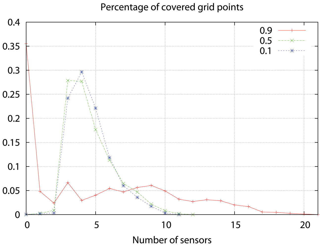
| >1 [0.99973%] | >2 [0.99777%] | >3 [0.99448%] | >4 [0.75258%] | >5 [0.45608%] | ||
| θ = 0.1 | sinc. < 1ms | 64.40 | 64.40 | 64.40 | 5.30 | 1.60 |
| sinc. 1ms | 78.00 | 66.90 | 73.90 | 5.50 | 0.00 | |
| sinc. 10ms | 76.90 | 90.70 | 73.40 | 13.60 | 3.90 | |
| >1 [0.99988%] | >2 [0.99730%] | >3 [0.98856%] | >4 [0.70991%] | >5 [0.43301%] | ||
| θ = 0.5 | sinc. < 1ms | 139.20 | 138.90 | 123.50 | 8.30 | 0.00 |
| sinc. 1ms | 146.70 | 120.20 | 125.40 | 22.50 | 0.00 | |
| sinc. 10ms | 144.90 | 162.60 | 150.20 | 42.70 | 4.00 | |
| >1 [0.64476%] | >2 [0.59659%] | >3 [0.57273%] | >4 [0.50632%] | >5 [0.47687%] | ||
| θ = 0.9 | sinc. < 1ms | 114.00 | 66.80 | 20.20 | 11.00 | 1.50 |
| sinc. 1ms | 99.30 | 56.40 | 49.90 | 19.20 | 2.40 | |
| sinc. 10ms | 171.80 | 127.10 | 88.00 | 31.70 | 19.50 | |
© 2009 by the authors; licensee Molecular Diversity Preservation International, Basel, Switzerland. This article is an open access article distributed under the terms and conditions of the Creative Commons Attribution license (http://creativecommons.org/licenses/by/3.0/).
Share and Cite
González-Castaño, F.J.; Vales Alonso, J.; Costa-Montenegro, E.; López-Matencio, P.; Vicente-Carrasco, F.; Parrado-García, F.J.; Gil-Castiñeira, F.; Costas-Rodríguez, S. Acoustic Sensor Planning for Gunshot Location in National Parks: A Pareto Front Approach. Sensors 2009, 9, 9493-9512. https://doi.org/10.3390/91209493
González-Castaño FJ, Vales Alonso J, Costa-Montenegro E, López-Matencio P, Vicente-Carrasco F, Parrado-García FJ, Gil-Castiñeira F, Costas-Rodríguez S. Acoustic Sensor Planning for Gunshot Location in National Parks: A Pareto Front Approach. Sensors. 2009; 9(12):9493-9512. https://doi.org/10.3390/91209493
Chicago/Turabian StyleGonzález-Castaño, Francisco Javier, Javier Vales Alonso, Enrique Costa-Montenegro, Pablo López-Matencio, Francisco Vicente-Carrasco, Francisco J. Parrado-García, Felipe Gil-Castiñeira, and Sergio Costas-Rodríguez. 2009. "Acoustic Sensor Planning for Gunshot Location in National Parks: A Pareto Front Approach" Sensors 9, no. 12: 9493-9512. https://doi.org/10.3390/91209493