Multi-Line Fit Model for the Detection of Methane at ν2 + 2ν3 Band using Hollow-Core Photonic Bandgap Fibres


Abstract
:
1. Introduction
2. Theory of absorption spectroscopy
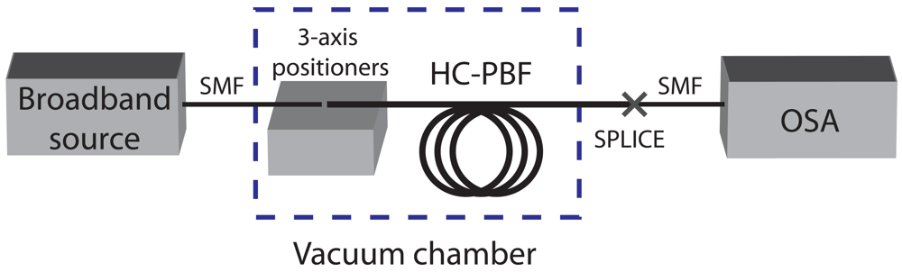
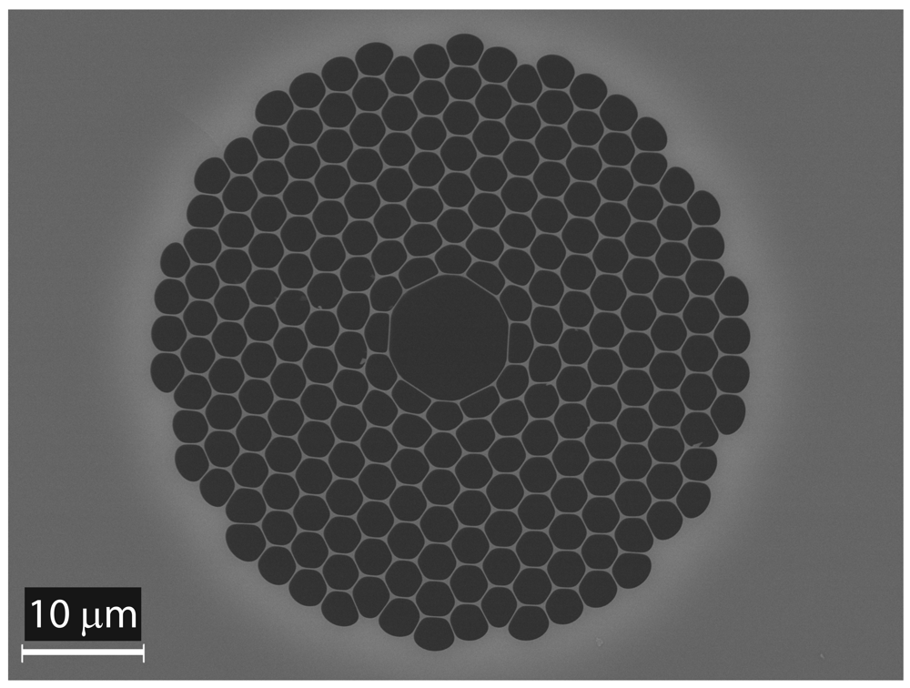
3. Experimental setup
4. Experimental results and Discussion
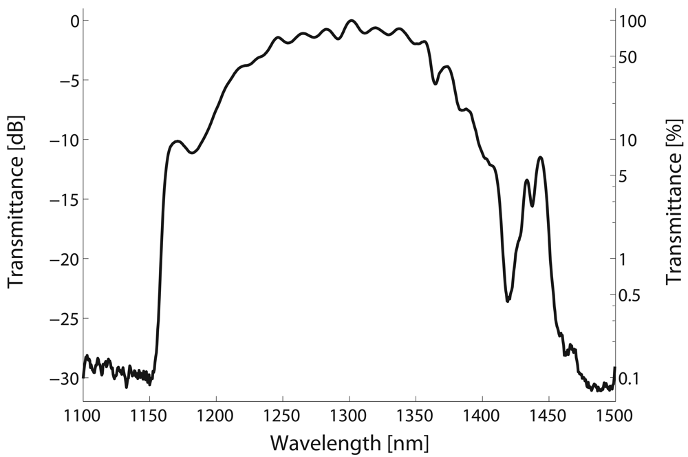
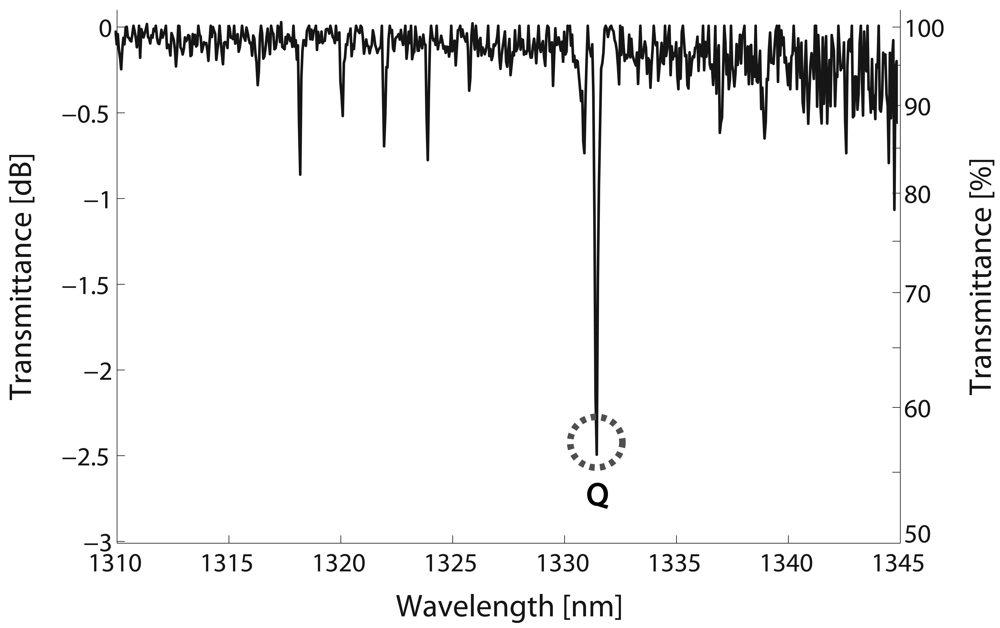
4.1. Selection of spectral lines
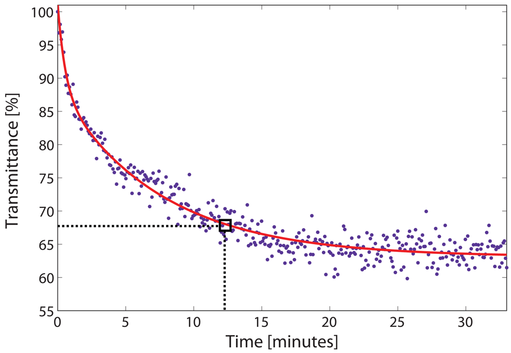
4.2. Filling dynamics of the HC-PBF
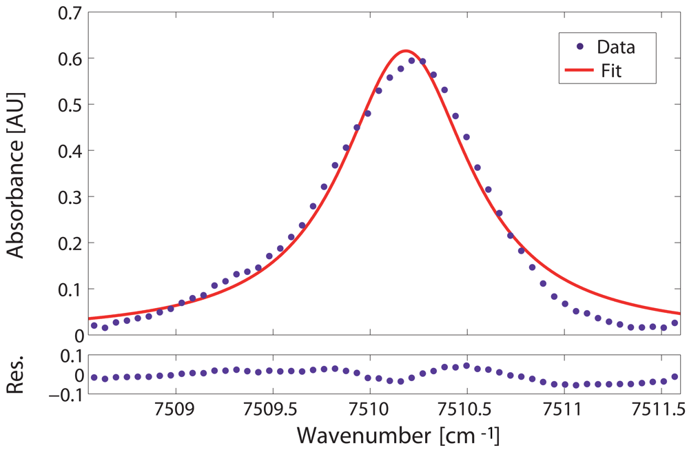
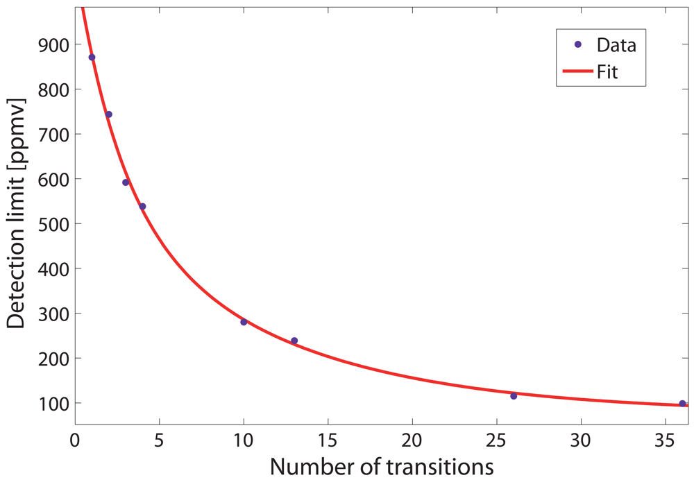
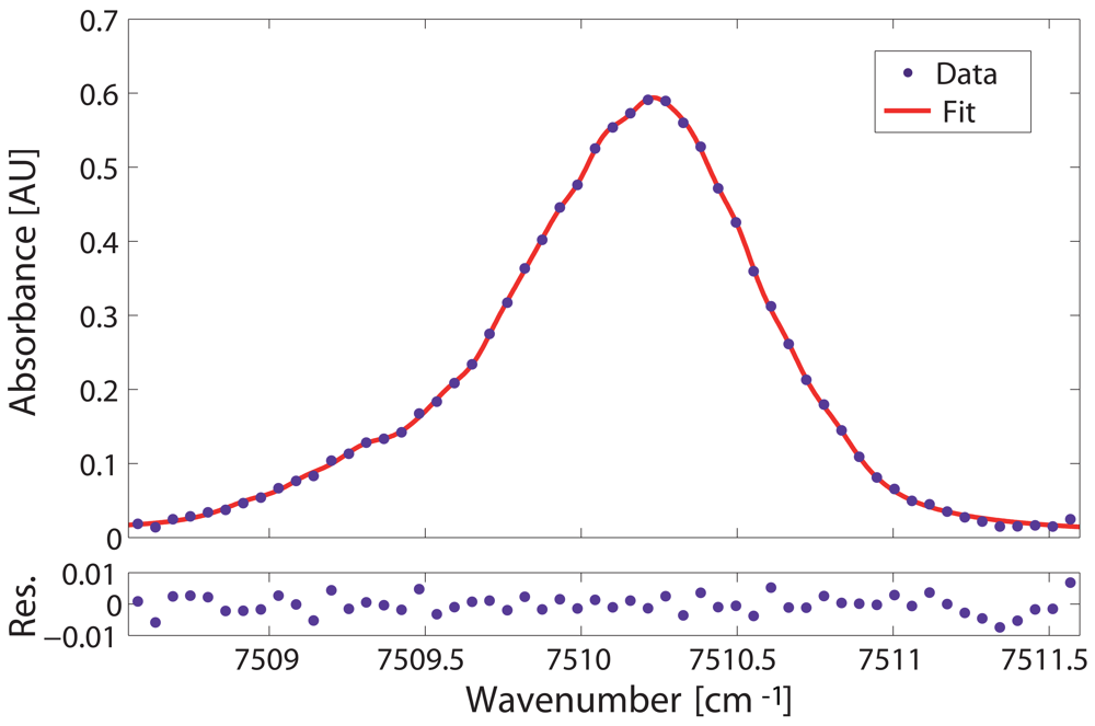
4.3. Data analysis and detection limit calculation
5. Conclusions
Acknowledgments
References and Notes
- Lopez-Higuera, J.M. Handbook of Optical Fibre Sensing Technology; Ed.; Ed. John Wiley & Sons: West Sussex, England, 2002. [Google Scholar]
- MNT gas sensor roadmap. Technical report; MNT Gas sensor forum, 2006. [Google Scholar]
- Culshaw, B.; Stewart, G.; Dong, F.; Tandy, C.; Moodie, D. Fibre optic techniques for remote spectroscopic methane detection. Sens. Actuators. B 1998, 51, 25–37. [Google Scholar]
- Stewart, G.; Jin, W.; Culshaw, B. Prospects for fibre-optic evanescent-field gas sensors using absorption in the near-infrared. Sens. Actuators. B 1997, 38-39, 42–47. [Google Scholar]
- Benabid, F. Hollow-core photonic bandgap fibre: new light guidance for new science and technology. Phil. Trans. R. Soc. A 2006, 364, 3439–3462. [Google Scholar]
- Petrovich, M.; van Brakel, A.; Poletti, F.; Musaka, K.; Austin, E.; Finazzi, V.; Petropoulos, P.; O'Driscoll, E.; Watson, M.; DelMonte, T.; Monro, T.M.; Dakin, J.P.; Richardson, D.J. Microstructured fibers for sensing applications. Du, Henry H., Ed.; In Proc. SPIE; Boston, USA, October 23C26 2005; Volume 6005, pp. 78–92. [Google Scholar]
- Ritari, T.; Tuominen, J.; Ludvigsen, H.; Petersen, J.C.; Sorensen, T.; Hansen, T.P.; Simonsen, H.R. Gas sensing using air-guiding photonic bandgap fibers. Opt. Express 2004, 12, 4080–4087. [Google Scholar]
- Kornaszewski, L.; Gayraud, N.; Stone, J.M.; Macpherson, W.; George, A.; Knight, J.C.; Hand, D.P.; Reid, D.T. Mid-infrared methane detection in a photonic bandgap fiber using a broadband optical parametric oscillator. Opt. Express 2007, 15, 11219–11224. [Google Scholar]
- Henningsen, J.; Hald, J.; Petersen, J.C. Saturated absorption in acetylene and hydrogen cyanide in hollow-core photonic bandgap fibers. Opt. Express 2005, 13, 10475–10482. [Google Scholar]
- Cubillas, A.M.; Hald, J.; Petersen, J.C. High resolution spectroscopy of ammonia in a hollow-core fiber. Opt. Express 2008, 16, 3976–3985. [Google Scholar]
- Tuominen, J.; Ritari, T.; Ludvigsen, H.; Petersen, J.C. Gas filled photonic bandgap fibers as wavelength references. Opt. Commun. 2005, 255, 272–277. [Google Scholar]
- Couny, F.; Light, P.; Benabid, F.; Russell, P.S.J. Electromagnetically induced transparency and saturable absorption in all-fiber devices based on 12C2H2-filled hollow-core photonic crystal fiber. Opt. Commun. 2006, 263, 28–31. [Google Scholar]
- Weldon, V.; O'Gorman, J.; Prez-Camacho, J.J.; Mcdonald, D.; Hegarty, J.; Corbett, B. Methane sensing with a novel micromachined single-frequency fabry-perot lased diode emitting at 1331 nm. IEEE Phot. Tech. Lett. 1997, 9, 357–359. [Google Scholar]
- Cubillas, A. M.; Lazaro, J.M.; Silva-Lopez, M.; Conde, O.M.; Petrovich, M. N.; Lopez-Higuera, J.M. Methane sensing at 1300 nm band with hollow-core photonic bandgap fibre as gas cell. Electron. Lett. 2008, 44, 403–404. [Google Scholar]
- Cubillas, A.M.; Silva-Lopez, M.; Lazaro, J. M.; Conde, O.M.; Petrovich, M.; Lopez-Higuera, J. M. Methane detection at 1670-nm band using a hollow-core photonic bandgap fiber and a multiline algorithm. Opt. Express 2007, 15, 17570–17576. [Google Scholar]
- Bransden, B. H.; Joachain, C. J. Physics of atoms and molecules, 2nd Ed. ed; Pearson education Ltd., Prentice Hall: N.J., April 2003. [Google Scholar]
- Thapa, R.; Knabe, K.; Corwin, K.L.; Washburn, B.R. Arc fusion splicing of hollow-core photonic bandgap fibers for gas-filled fiber cells. Opt. Express 2006, 14, 9576–9583. [Google Scholar]
- Rothman, L.S.; Jacquemart, D.; Barbe, A.; Benner, D.C.; Birk, M.; Brown, L.R.; Carleer, M.R.; Chackerian, C.; Chance, K.; Coudert, L.H.; Dana, V.; Devi, V.M.; Flaud, J. M.; Gamache, R.R.; Goldman, A.; Hartmann, J.M.; Jucks, K.W.; Maki, A.G.; Mandin, J.Y.; Massie, S.T.; Orphal, J.; Perrin, A.; Rinsland, C.P.; Smith, M.A.H.; Tennyson, J.; Tolchenov, R.N.; Toth, R.A.; Auwera, J.V.; Varanasi, P.; Wagner, G. The HITRAN 2004 molecular spectroscopic database. J. Quant. Spectrosc. Radiat. Transfer 2005, 96, 139–204. [Google Scholar]
- Henningsen, J.; Hald, J. Dynamics of gas flow in hollow core photonic bandgap fibers. Appl. Opt. 2008, 47, 2790–2797. [Google Scholar]
- Carvalho, J.P.; Magalhes, F.; Ivanov, O.V.; Frazo, O.; Arajo, F.M.; Ferreira, L.A.; Santos, J.L. Evaluation of coupling losses in hollow-core photonic crystal fibres. Proc. SPIE 2007, 6619, 66191V. [Google Scholar]
- Lazaro, J.M.; Cubillas, A.M.; Silva-Lopez, M.; Conde, O.M.; Petrovich, M.; Lopez-Higuera, J.M. Methane sensing using multiple-coupling gaps in hollow-core photonic bandgap fibers. 19th International Conference on Optical Fibre Sensors (Perth, Australia); 2008. [Google Scholar]
- Nagali, V.; Hanson, R.K. Design of a diode-laser sensor to monitor water vapour in high-pressure combustion gases. Appl. Opt. 1997, 36, 9518–9527. [Google Scholar]
- Gharavi, M.; Buckley, S.G. Diode laser absorption spectroscopy measurement of linestrengths and pressure broadening coefficients of the methane 2ν3 band at elevated temperatures. J. Mol. Spectrosc. 2005, 229, 78–88. [Google Scholar]
- Webber, M. E.; Kim, S.; Sanders, S. T.; Baer, D. S.; Hanson, R. K.; Ikeda, Y. In situ combustion measurements of CO2 by use of a distributed-feedback diode-laser sensor near 2.0 μm. Appl. Opt. 2001, 22, 821–828. [Google Scholar]


| Minimum Si [cm−1/(mol cm−2)] | Number of transitions | Detection limit [ppmv] | Computational time [s] |
|---|---|---|---|
| 16×10−23 | 1 | 870 | 0.113 |
| 14×10−23 | 2 | 744 | 0.121 |
| 10×10−23 | 3 | 592 | 0.131 |
| 8×10⁻²³ | 4 | 538 | 0.141 |
| 6×10⁻²³ | 10 | 280 | 0.177 |
| 4×10⁻²³ | 13 | 239 | 0.205 |
| 2×10⁻²³ | 26 | 115 | 0.347 |
| 10×10−24 | 36 | 98 | 0.431 |
© 2009 by the authors; licensee Molecular Diversity Preservation International, Basel, Switzerland. This article is an open access article distributed under the terms and conditions of the Creative Commons Attribution license (http://creativecommons.org/licenses/by/3.0/).
Share and Cite
Cubillas, A.M.; Lazaro, J.M.; Conde, O.M.; Petrovich, M.N.; Lopez-Higuera, J.M. Multi-Line Fit Model for the Detection of Methane at ν2 + 2ν3 Band using Hollow-Core Photonic Bandgap Fibres. Sensors 2009, 9, 490-502. https://doi.org/10.3390/s90100490
Cubillas AM, Lazaro JM, Conde OM, Petrovich MN, Lopez-Higuera JM. Multi-Line Fit Model for the Detection of Methane at ν2 + 2ν3 Band using Hollow-Core Photonic Bandgap Fibres. Sensors. 2009; 9(1):490-502. https://doi.org/10.3390/s90100490
Chicago/Turabian StyleCubillas, Ana M., Jose M. Lazaro, Olga M. Conde, Marco N. Petrovich, and Jose M. Lopez-Higuera. 2009. "Multi-Line Fit Model for the Detection of Methane at ν2 + 2ν3 Band using Hollow-Core Photonic Bandgap Fibres" Sensors 9, no. 1: 490-502. https://doi.org/10.3390/s90100490