A Novel Method for the Dynamic Coefficients Identification of Journal Bearings Using Kalman Filter


1
Tianjin Key Laboratory of Power Transmission and Safety Technology for New Energy Vehicles, School of Mechanical Engineering, Hebei University of Technology, Tianjin 300130, China
2
Centre for Efficiency and Performance Engineering, University of Huddersfield, Huddersfield HD1 3DH, UK
*
Author to whom correspondence should be addressed.
Sensors 2020, 20(2), 565; https://doi.org/10.3390/s20020565
Submission received: 2 December 2019
/
Revised: 14 January 2020
/
Accepted: 16 January 2020
/
Published: 20 January 2020
(This article belongs to the Section Physical Sensors)
Abstract
:The dynamic coefficients identification of journal bearings is essential for instability analysis of rotation machinery. Aiming at the measured displacement of a single location, an improvement method associated with the Kalman filter is proposed to estimate the bearing dynamic coefficients. Firstly, a finite element model of the flexible rotor-bearing system was established and then modified by the modal test. Secondly, the model-based identification procedure was derived, in which the displacements of the shaft at bearings locations were estimated by the Kalman filter algorithm to identify the dynamic coefficients. Finally, considering the effect of the different process noise covariance, the corresponding numerical simulations were carried out to validate the preliminary accuracy. Furthermore, experimental tests were conducted to confirm the practicality, where the real stiffness and damping were comprehensively identified under the different operating conditions. The results show that the proposed method is not only highly accurate, but also stable under different measured locations. Compared with the conventional method, this study presents a more than high practicality approach to identify dynamic coefficients, including under the resonance condition. With high efficiency, it can be extended to predict the dynamic behaviour of rotor-bearing systems.
1. Introduction
In a rotor-bearing system, the bearing dynamic coefficients affect the dynamic behaviour of the system directly, such as the critical speed, imbalance response, and stability performance. Many investigations based on the theoretical model have been carried out to calculate the dynamic coefficients [1,2,3,4]. However, the simplification in modeling inevitably leads to errors between the calculated and actual values. Thus, a high-accuracy identification method is necessary in terms of the assessment for the overall performance and operating conditions of the rotor system.
Many experimental identification methods have been developed to identify the bearing dynamic coefficients based on the model of the system and the measurement displacement, which are often designed based on the excitation methods, such as dynamic loads [5], impulse [6,7], and the imbalance mass [8]. Among these excitation methods, the imbalance mass, which has high accuracy and does not need extra devices, is more widely used in the identification of the bearing dynamic coefficients [9,10] and imbalance information [11,12]. Additionally, some optimization techniques, such as the equivalent dynamic load reconstruction [13], hybrid evolutionary algorithm [14], and the Bayesian inference [15], are combined with the imbalance excitation methods to improve the accuracy in bearing dynamic coefficients. Moreover, the ill-problems in the identification process are also a concern and should be avoided by combining the dynamic equations from the unbalance response and the proposed complementary equations [16].
For a flexible rotor-bearing system, the accuracy of the model-based identification method of the dynamic coefficients is sensitive to the system model and the displacement of the shaft at bearings. If the finite element model is perfect, and the displacement can be accurately measured, the actual dynamic coefficients can be identified directly. However, in real applications, the displacement of the shaft at bearings is very difficult to measure directly because the measured location cannot be installed at the bearing node in the finite element model. The measured displacement at the bearing housing also cannot be used to identify the bearing dynamic coefficients directly [5,6,11]. Therefore, to obtain the actual displacement of the shaft at bearings, a conventional method has been proposed and widely used, which is based on the linear interpolation to estimate the displacement of the shaft at both bearings using the measured displacements near every bearing location [9,10,17]. However, if the sensors are far away from the locations of bearings and only the displacement of the single location can be measured, the displacement of the shaft at bearing locations cannot be estimated by this method. For this problem, a double-section interpolation-iteration method, in which the initial dynamic coefficients are used to recover the displacement of the shaft at bearing locations to recalculate the dynamic coefficients, has been designed to identify the dynamic coefficients [18]. However, this method demands a large calculation space and easily causes divergent results.
The main challenge of previous model-based identification methods is to estimate the displacement of the shaft at bearings before the identification, especially when only the displacement of the single location can be measured. The Kalman filter is a system dynamic estimation algorithm which produces an estimation of unknown variables using a series of measurements observed over time containing statistical noise and other inaccuracies. This method has been used successfully in the estimation of the critical parameters of the system, such as force [19,20,21,22], structural damage diagnosis [23], inverse heat conduction [24], pore water electrical conductivity [25], and mobile-robot attitude [26] and dynamic state [27,28,29]. Additionally, compared with other algorithms, such as dual Kalman filter [30], join Kalman filter [31], and even recursive least squares (RLS) [32], Kalman filtering is not only easier to achieve for estimating the main parameters in the discrete-time dynamic system, but also can save computing time.
Therefore, in this paper, the Kalman filter is employed in estimating the displacement of the shaft at bearing locations using the measured displacement of the single location. With the estimated displacements and system model, which are transformed and reordered into the frequency domain, the bearing dynamic coefficients can be identified by the least-squares method [33]. Finally, numerical simulations are carried out to validate the accuracy of this method, considering the effect of the process noise covariance. Moreover, some comparisons between the proposed and conventional method are conducted, where the results show that this method has greater practicality and is more stable, including when the system is in the resonance condition.
The structure of this paper is organized as follows. Section 2 describes the experimental test rig and corresponding updated model of the system, which contains the flexible shaft, bearing supporting, and the discs. In Section 3, an identification method is presented. In Section 4, numerical simulations are carried out. Section 5 provides the experimental investigation, in which the imbalance mass is used to excite the flexible system supported by a pair of journal bearings. Section 6 presents the conclusion of the proposed method.
2. Test Rig and Rotor Modeling
2.1. Test Rig
The rotor-bearing test rig is shown in Figure 1. The shaft was supported by a pair of journal bearings (bearing 1 and bearing 2). Two steel discs were installed symmetrically on the shaft. The laser displacement sensors were used to measure the displacement of shaft in the horizontal and vertical directions, respectively. A three-phase electric motor connected the rotor through a flexible coupling. The rotational speed could be controlled by a variable frequency AC drive. The parameters of the test rig are given in Table 1.
2.2. Modeling
The corresponding finite element model of the test rig, as shown in Figure 2, was developed. The shaft was modeled by several mass nodes connected with Timoshenko beam elements [34]. Each of the shaft elements had two nodes. Each of the nodes had four degrees of freedom (DOF), including two translational and two rotational. Node 2 and node 10 represent bearing 1 and bearing 2, respectively. Node 4 and node 8 represent the discs’ locations.
The linear equation of motion for the system can be described as:
where MR, CR, GR, and KR are the global matrix of lumped masses and inertial, damping, gyroscopic, and stiffness matrices of the rotors, respectively. KB and CB are the stiffness and damping matrix, which are required to be identified. Ω is the rotation speed. f (t) is the imbalance force vector. , , and q (t) are vectors of acceleration, velocity, and displacements, respectively, which are written as
where n is the number of degrees of freedom, qB1 and qB2 are the displacement of the shaft at bearing 1 and 2 locations, respectively, xi and yi are the translational displacements in the horizontal and vertical, respectively, θxi and θyi are the rotational displacements in the horizontal and vertical, respectively. The imbalance mass was inputted into the model to develop the imbalance force fu, which is equal to:
where m is the imbalance mass, r is the distributing radius of the imbalance mass, ω = Ω is the imbalance excitation frequency, φ is the phase.
The finite element model was then updated to improve its precision. Firstly, the experimental modal parameters and the frequency responses of the shaft with discs were measured. Then, the mass matrix of the model was optimized by the Nelder–Mead simplex optimization algorithm [35]. Finally, the updated model was verified by the comparison of the frequency responses between the calculation and measurement. The theoretical first-four order mode shapes are shown in Figure 3. The modal frequencies obtained from the initial model, the updated model, and measured values are given in Table 2. It can be found that the modal frequencies of the updated finite element model were closer to the measured data than the initial model. Therefore, the finite element model was updated successfully.
3. Proposed Method
Most identification methods of the bearing dynamic coefficients are based on the estimated displacement of the shaft at bearing locations. Therefore, an improved identification method based on the Kalman filter is proposed using the measured displacement from a single location to identify the bearing dynamic coefficients. Firstly, applying the system parameters to the model of the system, the actual displacements of both bearings are estimated by Kalman filter using the measured displacement of the single location. Secondly, using the estimated displacement, the actual dynamic coefficients are identified by the least-squares method. The flowchart of the proposed method is given in Figure 4.
3.1. Displacement Estimation
Generally, the accuracy of the identification method mainly depends on the displacement of the shaft at bearing locations, because it is very difficult to measure directly. Therefore, in this section, based on the Kalman filter, the displacement of the shaft at bearing locations was estimated using a single measurement location outside of the bearing. To achieve the Kalman filter in high accuracy, the theoretical dynamic coefficients of different rotation speeds, which are close to the actual value and calculated by the perturbation method [36], were applied to the model of the system.
The Kalman filter requires the state-space representation of the governing equation of the system and Equation (1) should be transformed as:
where is the state vectors, Ac is the system matrix, Bc is the input matrix, Gc is the output influence matrix, Y(t) represents the measurement vector.
where KB_theoretical and CB_theoretical are the theoretical values of the stiffness and damping matrix, respectively.
Then, discretize (5) and (6) over the time interval of the ∆t, as given in the following,
where k is the time index, X(k) is the state vector, f(k) is the force vector, Z(k) denotes the measurement vector, A is the state transition matrix, B is the input matrix, G represents the output influence matrix, and W(k) and V(k) are the system and measurement noise vectors, which are assumed to be zero mean and white noise with variance Q and R, respectively.
Based on the Kalman filter, qx,B1, the displacement of the shaft at bearing 1 in the horizontal direction was estimated by the following three steps.
Step 1: State predicted.
Step 2: Kalman gain calculated.
Step 3: State updated.
where Gx, B1 is the output influence matrix corresponding to the bearing 1 node at the horizontal direction and can be obtained from G, is the predicted state vectors, denotes the updated state, which is the estimated displacement of qx, B1, P(k/k−1) and P(k/k) represent the predicted and updated covariance matrix, respectively, S(k) is the innovation covariance matrix, Kg is the Kalman gain, Z(k) represents the innovation matrix.
After the above calculation, the displacement of the shaft at bearing 1 location in the horizontal direction (qx, B1) has been obtained. Additionally, the displacement of the shaft at bearing 1 in the vertical direction (qy, B1), and bearing 2 in both directions (qx, B2, qy, B2) can be estimated by the same procedure.
3.2. Bearing Dynamic Coefficients Identification
The displacements of the shaft at both bearing locations can be determined, as shown in the last section. With the estimated displacement, the bearing dynamic coefficients can be identified in the following process.
In this study, the identification method was designed with the system model in the frequency domain. After applying the Fourier transform, Equation (1) can be expressed as:
and the transfer function between imbalance extrication and displacement is:
With:
Thus, the equation of the motion of the rotor-bearing system can be represented by HR(Ω) and HB(Ω) and rewritten as below:
where qu is the displacement vectors of the system, which is in the complex form and caused by the imbalance force.
To identify the dynamic coefficients directly, the algebraic system of Equation (23) was reordered by the use of matrix operation to bring the estimated displacements of the shaft at both bearing locations into the upper rows. The displacement vector can be rewritten as:
where the vector zu represents the vector of unknown rotor displacements. zB1 and zB2 represent the estimated displacement vectors of the shaft at bearing locations, respectively, as:
The system of Equation (23) can be rewritten and shown as:
With:
In order to calculate conveniently, is partitioned into a sub-matrix like below:
where the displacement of the shaft at bearing locations and the imbalance force vector can be measured and calculated directly. Thus, the third row of Equation (29), zu can be expressed as:
Then, from the first and second row of Equation (29), the following equations can be obtained:
Since the zu can be calculated from Equation (30) and the fB1 and fB2 are known, the bearing dynamic coefficients can be identified by:
where E is the displacement matrix of both bearings, β is the parameters matrix of the bearing dynamic coefficients, which are required to be identified, and D is the system matrix that contains fB1 and fB2.
Finally, the bearing dynamic coefficients can be calculated by the least-squares method in one operation, as:
4. Simulations
In this section, to validate the accuracy of the proposed method, the numerical simulations are conducted, where the effect of the variance Q for the bearing dynamic coefficients is considered and discussed.
Firstly, the imbalance mass was added to generate the corresponding imbalance force shown in Equation (4). The assumed dynamic coefficients of both bearings at rotation speeds from 600 to 4800 rpm were added to the model to generate the simulation displacement and achieve the Kalman filter, in which the dynamic coefficients of both bearings were the same value. During the range of the rotation speeds, the displacement of each node could be obtained by the simulation calculation. Secondly, based on the Kalman filter, the displacements of shafts at the bearing locations were estimated by the displacement of node 6, where the estimated displacements were validated by the actual value of the bearing nodes 2 and 10. Finally, with the estimated displacement, the stiffness and damping coefficients of both bearings were identified and compared with the assumed values. The details of the imbalance mass are given in Table 3.
The amplitude and phase of the estimated displacement during the range of the rotation speeds are shown in Figure 5 and Figure 6. The amplitude of bearing 2 was larger than the bearing 1 because the imbalance mass was added to disc 2 (node 8), which was close to bearing 2. To validate the estimation results, the actual displacements of shafts at the bearing locations (node 2 and 10) were also given in the following. It can be found that the estimated values matched quite well with the actual value, especially when the variance Q was less than 1 × 10⁻¹⁶.
Using the estimated displacement of shafts at the bearing locations, the dynamic coefficients of both bearings were identified during the range of the rotation speeds. The identified stiffness and damping coefficients of both bearings are presented as the same results. Therefore, the dynamic coefficients of bearing 2 are given in Figure 7 and Figure 8. From the results, it can be seen that all of the identified dynamic coefficients under different variances Q agreed well with the assumed coefficients, especially when the variance Q was 1 × 10⁻¹⁸. Therefore, it can be concluded that, theoretically, the presented method has high confidence in the identification of dynamic coefficients.
5. Experimental Analysis
The accuracy of the proposed method was preliminarily validated in the last section. In this section, based on the flexible test rig shown in Figure 2, the identification procedure used the measured displacement for the three cases of locations to determine the stiffness and damping coefficients of a pair of journal bearings.
5.1. Experimental Description
The imbalance masses as an excitation force were added to disc 1 and disc 2. The laser displacement sensors were used to measure the displacement of the shaft. In this paper, at the range of the rotation speed from 600 rpm to 2200 rpm, the displacement of the three different locations, 1, 2, and 3, were measured and used to identify the stiffness and damping coefficients. The details of the displacement sensors are shown in Figure 9. The parameters of the imbalance mass are given in Table 4.
To validate the accuracy and practicality of the proposed method, the displacements of the bearing locations and dynamic coefficients were also identified based on the conventional method [17], which requires the measured displacements of the two locations near the bearings. The conventional method is widely used but is not suitable for complex structures because it is sensitive to the selection of the measured locations. The comparisons between the proposed and conventional method are given in Section 5.2.
5.2. Results and Discussions
The amplitude and phase of the shaft displacement at both bearing locations were estimated and are provided in Figure 10 and Figure 11. The amplitude had an evident increase from 1600 to 1900 rpm because of the first-order critical speed. Over the whole range of the rotation speed, it can be seen that the estimated amplitude and phase under different measured displacements agreed well with the conventional method, including at the first-order critical speed.
With the estimated displacement of bearings, the stiffness and damping coefficients of both bearings were identified. The dynamic coefficients of bearing 1 are shown in Figure 12 and Figure 13. As the rotation speeds increased, the direct stiffness coefficient Kyy had significant decreases, whereas Kxx remained almost constant. The cross-coupled stiffness coefficients Kxy and Kyx were negative and had slight increases over the speed range considered. Besides this, the direct damping coefficients Cxx remained nearly invariant. The cross-coupled damping coefficients (Cxy, Cyx) were similar and smaller than the direct damping coefficients Cyy, which decreased throughout the speed range. From the results, it can be seen that this method not only has a similar accuracy to the conventional method, but is also stable under different measured locations. Compared with the conventional method, this method requiring fewer measured locations makes it more practical for complex structures.
In Figure 14 and Figure 15, the identified stiffness and damping coefficients of bearing 2 are provided. Since the machine was a symmetry structure supported by two same journal bearings, the dynamic coefficients of both bearings were similar.
From the comparisons, it can be seen that the identified dynamic coefficients of both bearings obtained satisfying accuracy, including under the resonance condition. Additionally, the proposed method was more flexible in the section of the measured locations because it is stable under different measured locations. Therefore, this method can improve the practicality for the identification of dynamic coefficients in complex structures.
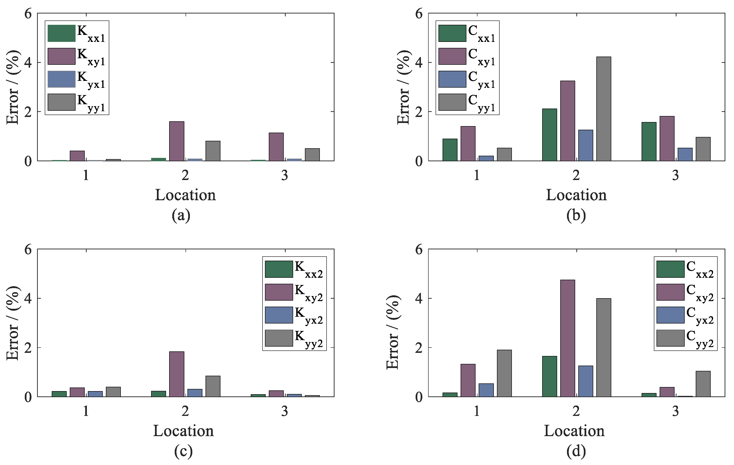
To investigate the influencing features of the measured locations, the errors between the proposed and conventional method were determined by:
Therefore, the errors of dynamic coefficients under different measured locations were calculated and are presented in Figure 16. From the results, it can be seen that the accuracy of the identification was not affected by the position of the sensor location. Compared with the conventional method, it can be believed that the proposed method, which only requires the displacement of the single location, is more practical and stable, especially in stiffness identification.
In the process of experimental identification, the sampling frequency was 10,240 Hz., while the number of data points was 20,480. The computing time was around 4.402008 s, including estimating the displacement and dynamic coefficients of both bearings. According to the identification results, the proposed method can be carried out for identification in real-time.
6. Conclusions
In this paper, the identification of dynamic coefficients was comprehensively investigated in a flexible rotor-journal bearing system. An improvement method was proposed to accurately estimate bearing dynamic coefficients from the measured displacement of a single location.
The procedure of the identification based on the updated finite element model was presented, where the Kalman filter was applied to estimate the actual displacement at the shaft of both bearing locations using the measured displacement from a single location. To validate the effectiveness and accuracy, numerical simulations under different process noise variances were carried out. The results show that all of the identified coefficients matched quite well with the assumed coefficients used for generating the simulation displacements. Furthermore, with the proposed method, experimental tests were also undertaken to identify the dynamic coefficients, including the stiffness and damping parameters. The high precision of the identified coefficients, particularly the stiffness, was confirmed under the operating conditions. Compared with the conventional method, this method is not only stable, including in the resonance condition, but more practical for complex systems. Additionally, the proposed method can achieve the identification of dynamic coefficients in real-time.
It can be concluded that this study can serve as a more efficient and reliable tool for monitoring the stable work of the rotor-bearing system, together with the fault diagnosis.
Author Contributions
All authors contributed to this work. Conceptualization, Y.K., Formal analysis, D.Z., Investigation, Y.K., Methodology, F.G., Validation, Z.S., Writing—original draft, D.Z., Writing—review and editing, H.Z. All authors have read and agreed to the published version of the manuscript.
Funding
This research was financially supported by the National Natural Science Foundation of China (Grant no. 51875166,51705127,51605133), Hebei Provincial International Science and Technology Cooperation Program of China (Grant no. 17394303D), China Scholarship Council (201906700007).
Conflicts of Interest
The authors declare no conflict of interest.
References
- Snyder, T.; Braun, M. Comparison of Perturbed Reynolds Equation and CFD Models for the Prediction of Dynamic Coefficients of Sliding Bearings. Lubricants 2018, 6, 5. [Google Scholar] [CrossRef] [Green Version]
- Li, Q.; Zhang, S.; Ma, L. Stiffness and damping coefficients for journal bearing using the 3D transient flow calculation. J. Mech. Sci. Technol. 2017, 31, 2083–2091. [Google Scholar] [CrossRef]
- Dyk, Š.; Rendl, J.; Byrtus, M. Dynamic coefficients and stability analysis of finite-length journal bearings considering approximate analytical solutions of the Reynolds equation. Tribol. Int. 2019, 130, 229–244. [Google Scholar] [CrossRef]
- Merelli, C.E.; Barilá, D.O.; Vignolo, G.G.; Quinzani, L.M. Dynamic Coefficients of Finite Length Journal Bearing. Evaluation Using a Regular Perturbation Method. Int. J. Mech. Sci. 2019, 151, 251–262. [Google Scholar] [CrossRef] [Green Version]
- Tiwari, R.; Lees, A.W.; Friswell, M.I. Identification of Speed-Dependent Bearing Parameters. J. Sound Vib. 2002, 254, 967–986. [Google Scholar] [CrossRef] [Green Version]
- Tiwari, R.; Chakravarthy, V. Simultaneous identification of residual imbalances and bearing dynamic parameters from impulse responses of rotor–bearing systems. Mech. Syst. Signal Process. 2006, 20, 1590–1614. [Google Scholar] [CrossRef]
- Qiu, Z.L.; Tieu, A.K. Identification of sixteen force coefficients of two journal bearings from impulse responses. Wear 1997, 212, 206–212. [Google Scholar] [CrossRef]
- Tiwari, R.; Lees, A.W.; Friswell, M.I. Identification of dynamic bearing parameters: A review. Shock Vib. Dig. 2004, 36, 99–124. [Google Scholar] [CrossRef]
- Tieu, A.K.; Qiu, Z.L. Identification of sixteen dynamic coefficients of two journal bearings from experimental imbalance response. Wear 1994, 177, 63–69. [Google Scholar] [CrossRef]
- Xu, Y.; Zhou, J.; Di, L.; Zhao, C. Active magnetic bearings dynamic parameters identification from experimental rotor unbalance response. Mech. Syst. Signal Process. 2016, 83, 228–240. [Google Scholar] [CrossRef]
- Tiwari, R.; Chakravarthy, V. Simultaneous estimation of the residual imbalance and bearing dynamic parameters from the experimental data in a rotor-bearing system. Mech. Mach. Theory 2009, 44, 792–812. [Google Scholar] [CrossRef]
- Han, F.; Guo, X.; Gao, H. Bearing parameter identification of rotor-bearing system based on Kriging surrogate model and evolutionary algorithm. J. Sound Vib. 2013, 332, 2659–2671. [Google Scholar] [CrossRef]
- Li, K.; Liu, J.; Han, X. Identification of oil-film coefficients for a rotor-journal bearing system based on equivalent load reconstruction. Tribol. Int. 2016, 104, 285–293. [Google Scholar] [CrossRef] [Green Version]
- Kim, Y.H.; Yang, B.S.; Tan, A.C.C. Bearing parameter identification of rotor–bearing system using clustering-based hybrid evolutionary algorithm. Struct. Multidiscip. Optim. 2007, 33, 493–506. [Google Scholar] [CrossRef]
- Tyminski, N.C.; Tuckmantel, F.W.S.; Cavalca, K.L.; De Castro, H.F. Bayesian inference applied to journal bearing parameter identification. J. Braz. Soc. Mech. Sci. Eng. 2017, 39, 2983–3004. [Google Scholar] [CrossRef]
- Chen, C.; Jing, J.; Cong, J.; Dai, Z. Identification of dynamic coefficients in circular journal bearings from imbalance response and complementary equations. J. Eng. Tribol. 2019, 233, 1016–1028. [Google Scholar]
- Santiago, O.D.; Andres, L.S. Experimental Identification of Bearing Dynamic Force Coefficients in a Flexible Rotor—Further Developments. Tribol. Lubr. Technol. 2007, 50, 114–126. [Google Scholar] [CrossRef]
- Li, Q.; Wang, W.; Weaver, B. Model-Based Interpolation-Iteration Method for Bearing Coefficients Identification of Operating Flexible Rotor-Bearing System. Int. J. Mech. Sci. 2017, 131, 471–479. [Google Scholar] [CrossRef]
- Ma, C.K.; Lin, D.C. Input forces estimation of a cantilever beam. Inverse Probl. Eng. 2000, 8, 511–528. [Google Scholar] [CrossRef]
- Loh, C.H.; Yang, J.N. Input force identification using Kalman filter techniques: Application to soil-pile interaction. Int. Soc. Opt. Eng. 2008, 6932, 1–12. [Google Scholar]
- Song, X.; Zhang, Y.; Liang, D. Load Identification for a Cantilever Beam Based on Fiber Bragg Grating Sensors. Sensors 2017, 17, 1733. [Google Scholar] [CrossRef] [PubMed] [Green Version]
- Shrivastava, A.; Mohanty, A.R. Estimation of single plane unbalance parameters of a rotor-bearing system using Kalman filtering based force estimation technique. J. Sound Vib. 2018, 418, 184–199. [Google Scholar] [CrossRef]
- Gao, F.; Lu, Y. A Kalman-filter based time-domain analysis for structural damage diagnosis with noisy signals. J. Sound Vib. 2006, 297, 916–930. [Google Scholar] [CrossRef]
- Pan, C.T.; Ji, C.; Li, W.F.; Wen, T.H. An input estimation approach to on-line two-dimensional inverse heat conduction problems. Numer. Heat Transf. 1996, 29, 345–363. [Google Scholar]
- Aljoumani, B.; Sanchez-Espigares, J.; Wessolek, G. Estimating Pore Water Electrical Conductivity of Sandy Soil from Time Domain Reflectometry Records Using a Time-Varying Dynamic Linear Model. Sensors 2018, 18, 4403. [Google Scholar] [CrossRef] [PubMed] [Green Version]
- Odry, A.; Fuller, R.; Rudas, I.J.; Odry, P. Kalman filter for mobile-robot attitude estimation: Novel optimized and adaptive solutions. Mech. Syst. Signal Process. 2018, 110, 569–589. [Google Scholar] [CrossRef]
- Battistelli, G.; Chisci, L. Stability of consensus extended Kalman filter for distributed state estimation. Automatica 2016, 68, 169–178. [Google Scholar] [CrossRef]
- Azam, S.E.; Chatzi, E.; Papadimitriou, C. A dual Kalman filter approach for state estimation via output-only acceleration measurements. Mech. Systems Signal Process. 2015, 60–61, 866–886. [Google Scholar] [CrossRef]
- Karimipour, H.; Dinavahi, V. Extended Kalman Filter-Based Parallel Dynamic State Estimation. IEEE Trans. Smart Grid 2015, 6, 1539–1549. [Google Scholar] [CrossRef]
- Manganiello, P.; Ricco, M.; Petrone, G.; Monmasson, E.; Spagnuolo, G. Dual-Kalman-filter-based identification and real-time optimization of PV systems. IEEE Trans. Ind. Electron. 2015, 62, 7266–7275. [Google Scholar] [CrossRef]
- Gao, S.; Liu, Y.; Wang, J. The Joint Adaptive Kalman Filter (JAKF) for Vehicle Motion State Estimation. Sensors 2016, 16, 1103. [Google Scholar] [CrossRef] [PubMed] [Green Version]
- Reichbach, N.; Kuperman, A. Recursive-Least-Squares-Based Real-Time Estimation of Supercapacitor Parameters. IEEE Trans. Energy Convers. 2016, 31, 1–3. [Google Scholar] [CrossRef]
- Zhao, S.X.; Zhou, H.; Meng, G.; Zhu, J. Experimental identification of linear oil-film coefficients using least-mean-square method in time domain. J. Sound Vib. 2005, 287, 809–825. [Google Scholar] [CrossRef]
- Nelson, H.D. A Finite Rotating Shaft Element Using Timoshenko Beam Theory. J. Mech. Des. 1980, 102, 793–803. [Google Scholar] [CrossRef]
- Nelder, J.A.; Mead, R. A Simplex Method for Function Minimization. Comput. J. 1965, 7, 308–313. [Google Scholar] [CrossRef]
- Kim, H.; Jang, G.; Ha, H. A generalized Reynolds equation and its perturbation equations for fluid dynamic bearings with curved surfaces. Tribol. Int. 2012, 50, 6–15. [Google Scholar] [CrossRef]
Figure 1.
Rotor bearing system.

Figure 2.
Finite element model.

Figure 3.
Theoretical mode shapes of the shaft with discs.

Figure 4.
Flowchart of the proposed method.
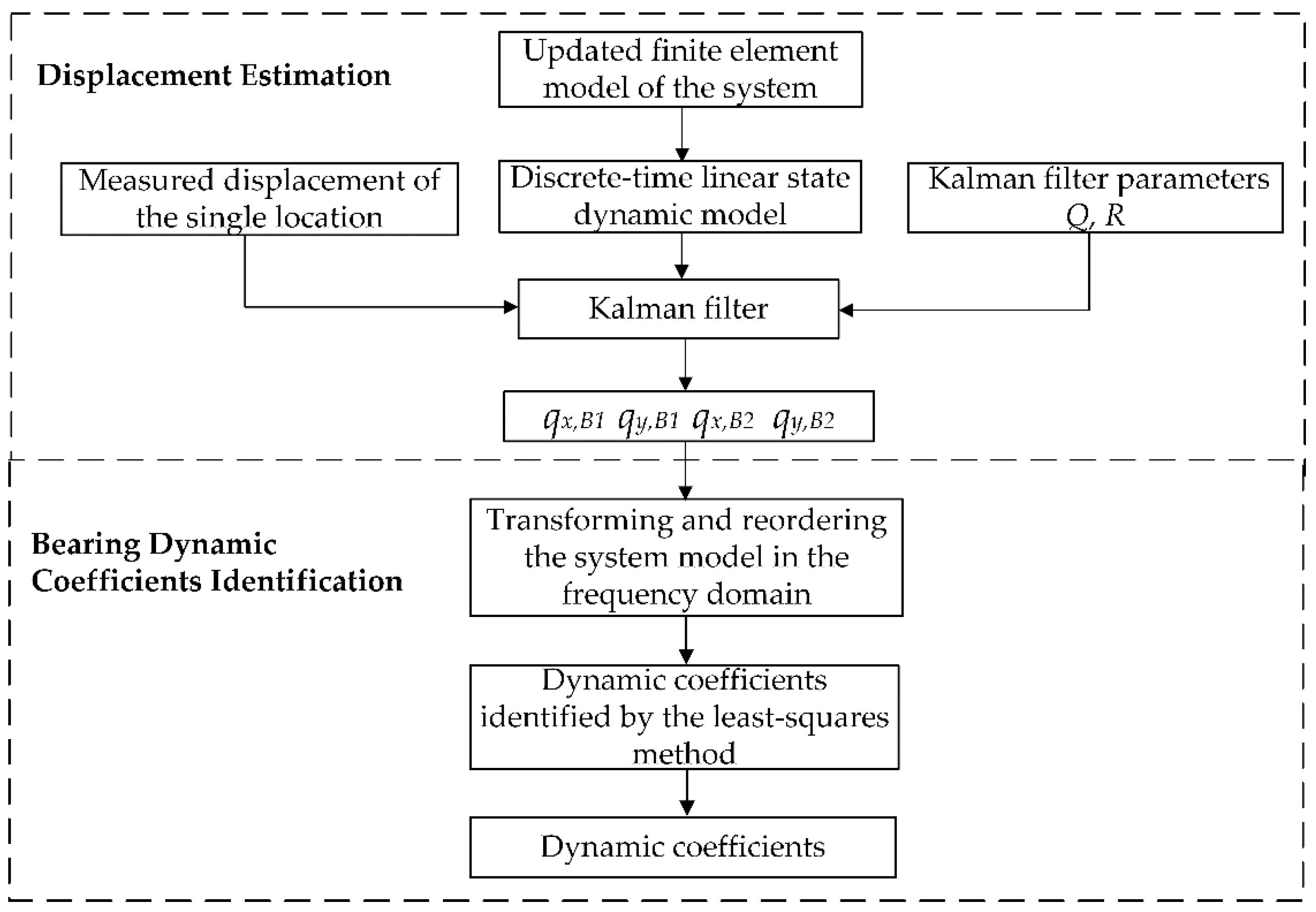
Figure 5.
Actual and estimated displacements of bearing 1; (a) amplitude of qx, B1; (b) phase of qx,B1; (c) Amplitude of qy, B1; (d) phase of qy, B1.
Figure 5.
Actual and estimated displacements of bearing 1; (a) amplitude of qx, B1; (b) phase of qx,B1; (c) Amplitude of qy, B1; (d) phase of qy, B1.
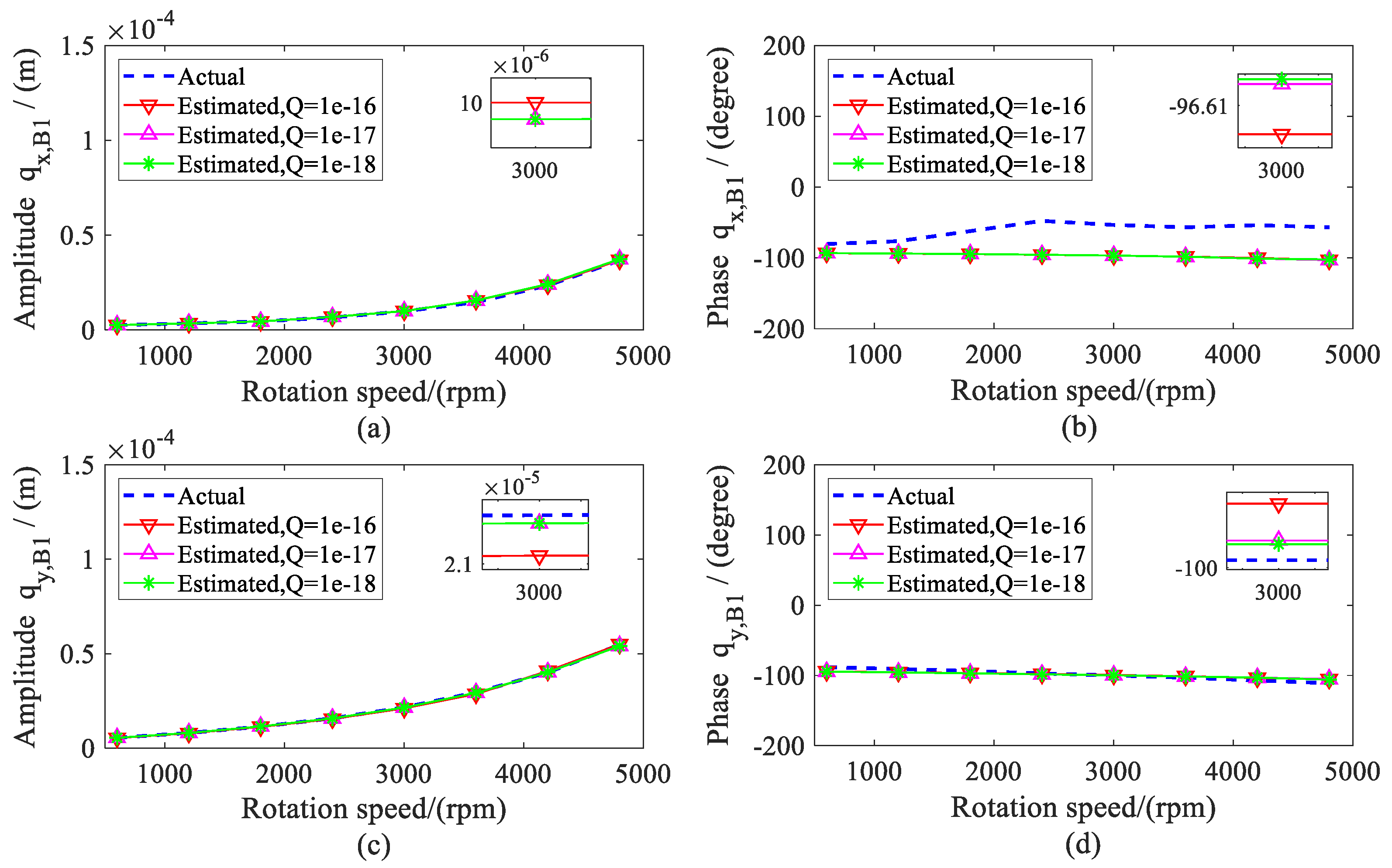
Figure 6.
Actual and estimated displacements of bearing 2. (a) amplitude of qx, B2; (b) phase of qx,B2; (c) amplitude of qy, B2; (d) phase of qy, B2.
Figure 6.
Actual and estimated displacements of bearing 2. (a) amplitude of qx, B2; (b) phase of qx,B2; (c) amplitude of qy, B2; (d) phase of qy, B2.
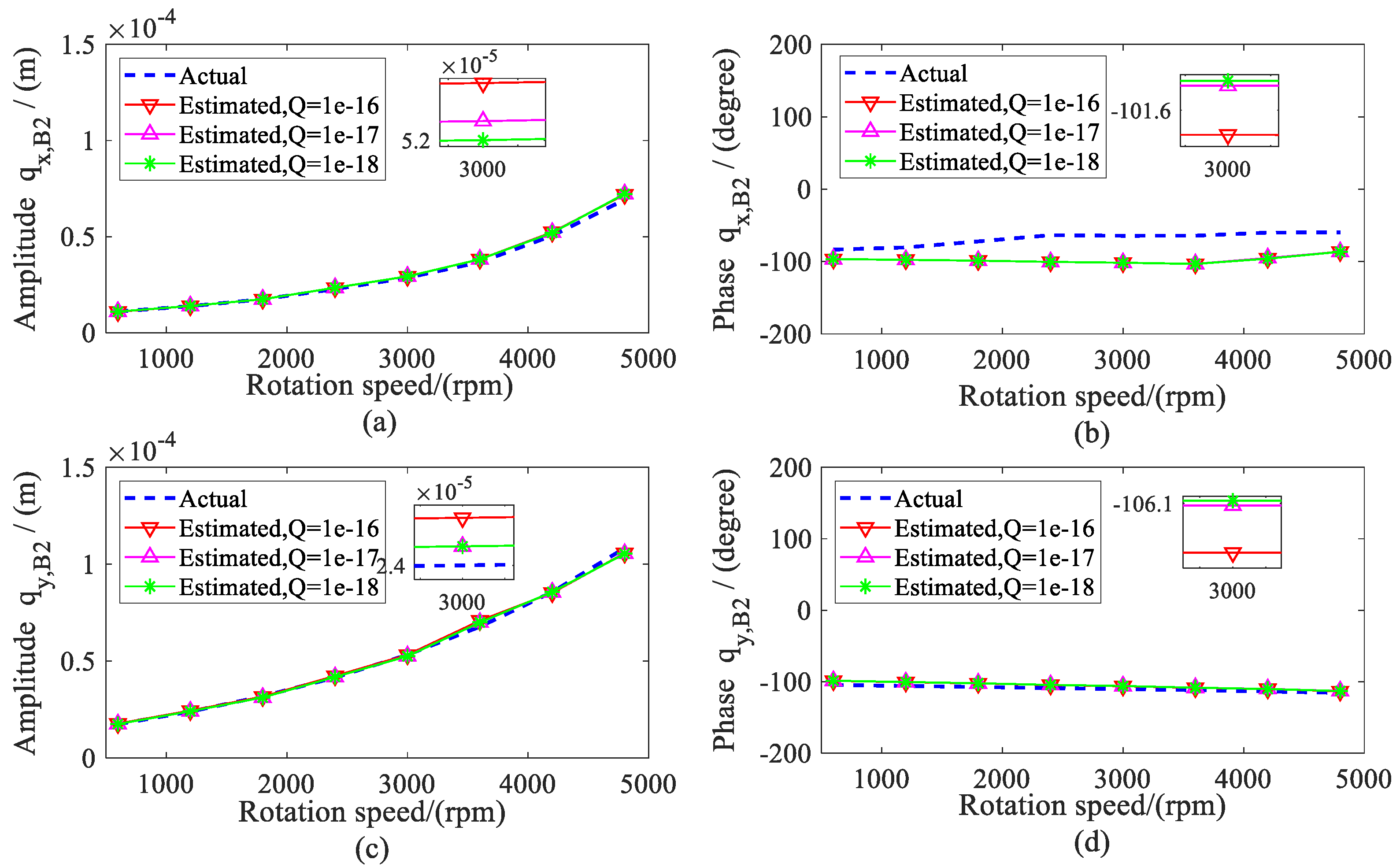
Figure 7.
Assumed and identified stiffness coefficients of bearing 2 versus rotation speed; (a) direct stiffness coefficient Kxx; (b) cross-coupled stiffness coefficient Kxy; (c) cross-coupled stiffness coefficients Kyx; (d) direct stiffness coefficients Kyy.
Figure 7.
Assumed and identified stiffness coefficients of bearing 2 versus rotation speed; (a) direct stiffness coefficient Kxx; (b) cross-coupled stiffness coefficient Kxy; (c) cross-coupled stiffness coefficients Kyx; (d) direct stiffness coefficients Kyy.
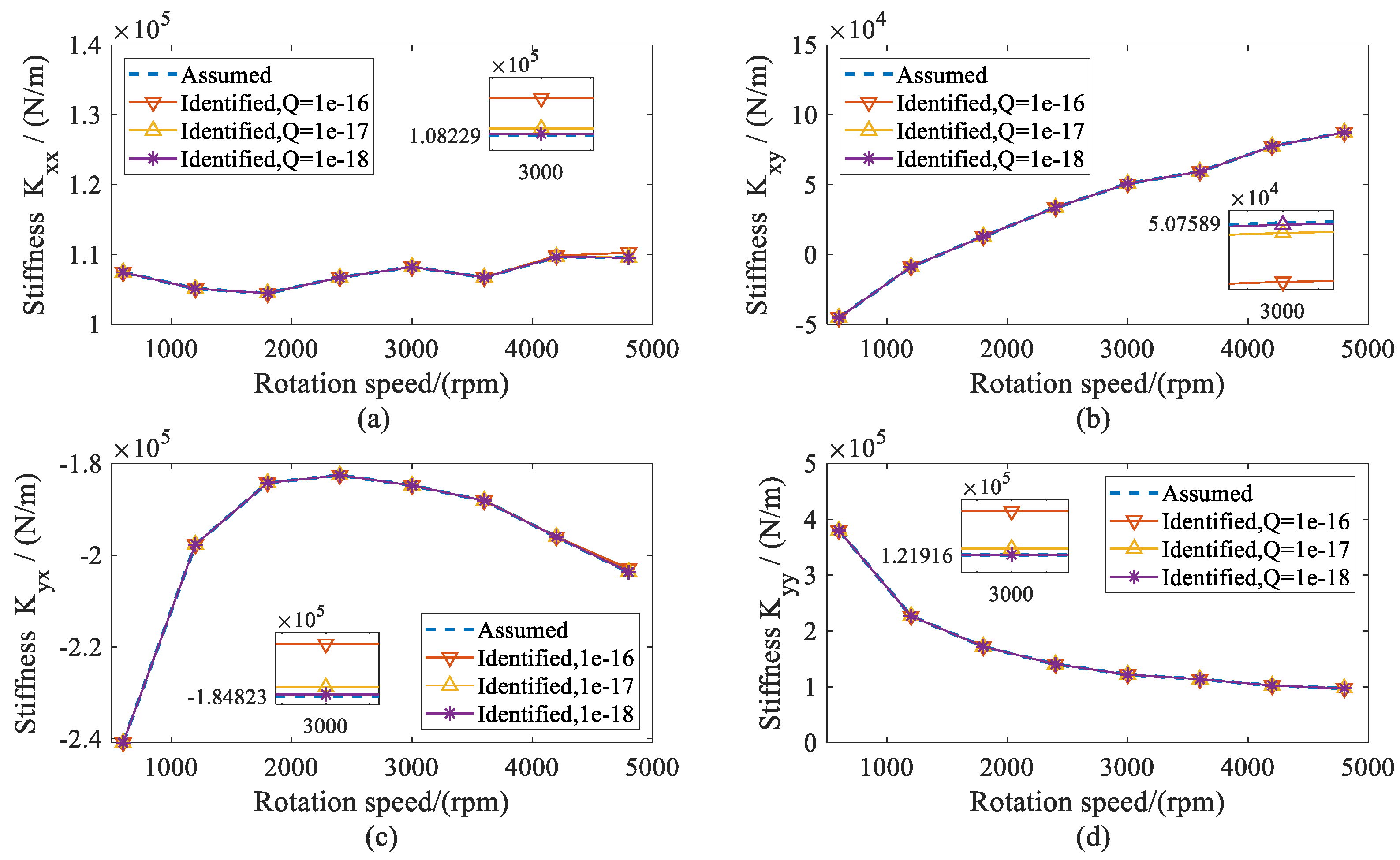
Figure 8.
Assumed and identified damping coefficients of bearing 2 versus rotation speed. (a) direct damping coefficients Cxx; (b) cross-coupled damping coefficients Cxy; (c) cross-coupled damping coefficients Cyx; (d) direct damping coefficients Cyy.
Figure 8.
Assumed and identified damping coefficients of bearing 2 versus rotation speed. (a) direct damping coefficients Cxx; (b) cross-coupled damping coefficients Cxy; (c) cross-coupled damping coefficients Cyx; (d) direct damping coefficients Cyy.

Figure 9.
The detail of the displacement sensor.
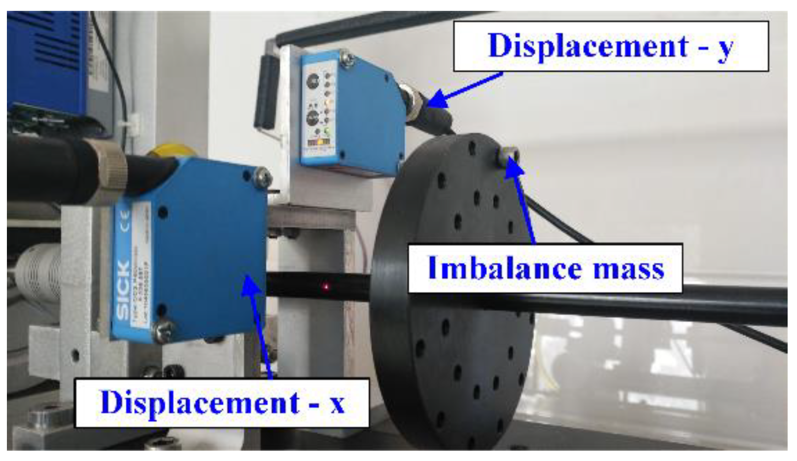
Figure 10.
Comparison for displacements of bearing 1. (a) amplitude of qx, B1; (b) phase of qx,B1; (c) amplitude of qy, B1; (d) phase of qy, B1.
Figure 10.
Comparison for displacements of bearing 1. (a) amplitude of qx, B1; (b) phase of qx,B1; (c) amplitude of qy, B1; (d) phase of qy, B1.
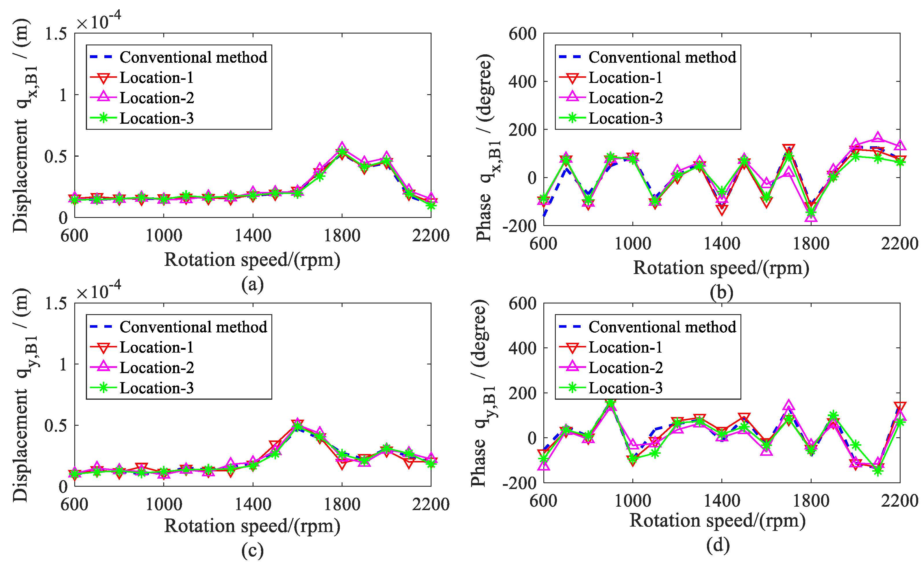
Figure 11.
Comparison for displacements of bearing 2. (a) amplitude of qx, B2; (b) phase of qx, B2; (c) amplitude of qy, B2; (d) phase of qy, B2.
Figure 11.
Comparison for displacements of bearing 2. (a) amplitude of qx, B2; (b) phase of qx, B2; (c) amplitude of qy, B2; (d) phase of qy, B2.
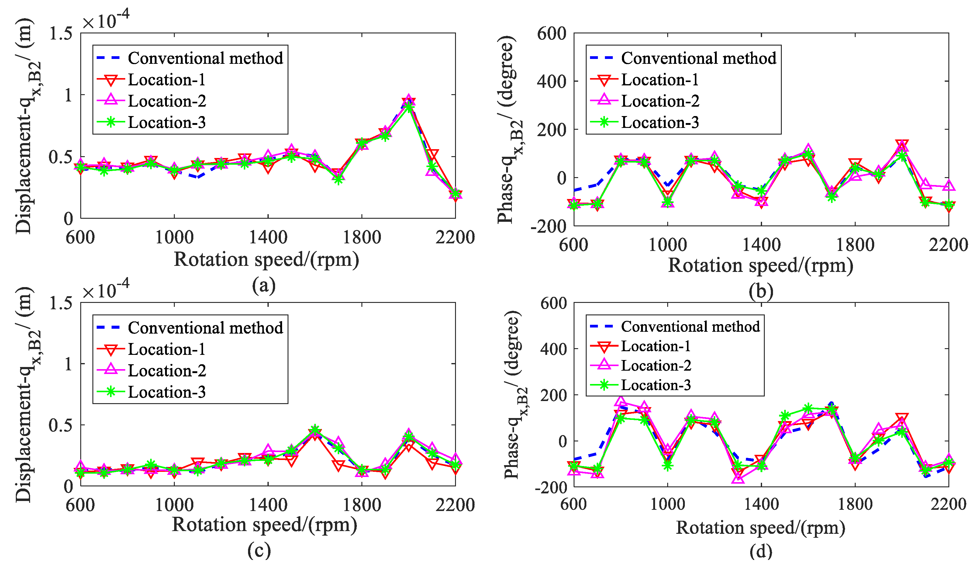
Figure 12.
Comparison for stiffness coefficients of bearing 1 versus rotation speed. (a) direct stiffness coefficient Kxx; (b) cross-coupled stiffness coefficient Kxy; (c) cross-coupled stiffness coefficients Kyx; (d) direct stiffness coefficients Kyy.
Figure 12.
Comparison for stiffness coefficients of bearing 1 versus rotation speed. (a) direct stiffness coefficient Kxx; (b) cross-coupled stiffness coefficient Kxy; (c) cross-coupled stiffness coefficients Kyx; (d) direct stiffness coefficients Kyy.
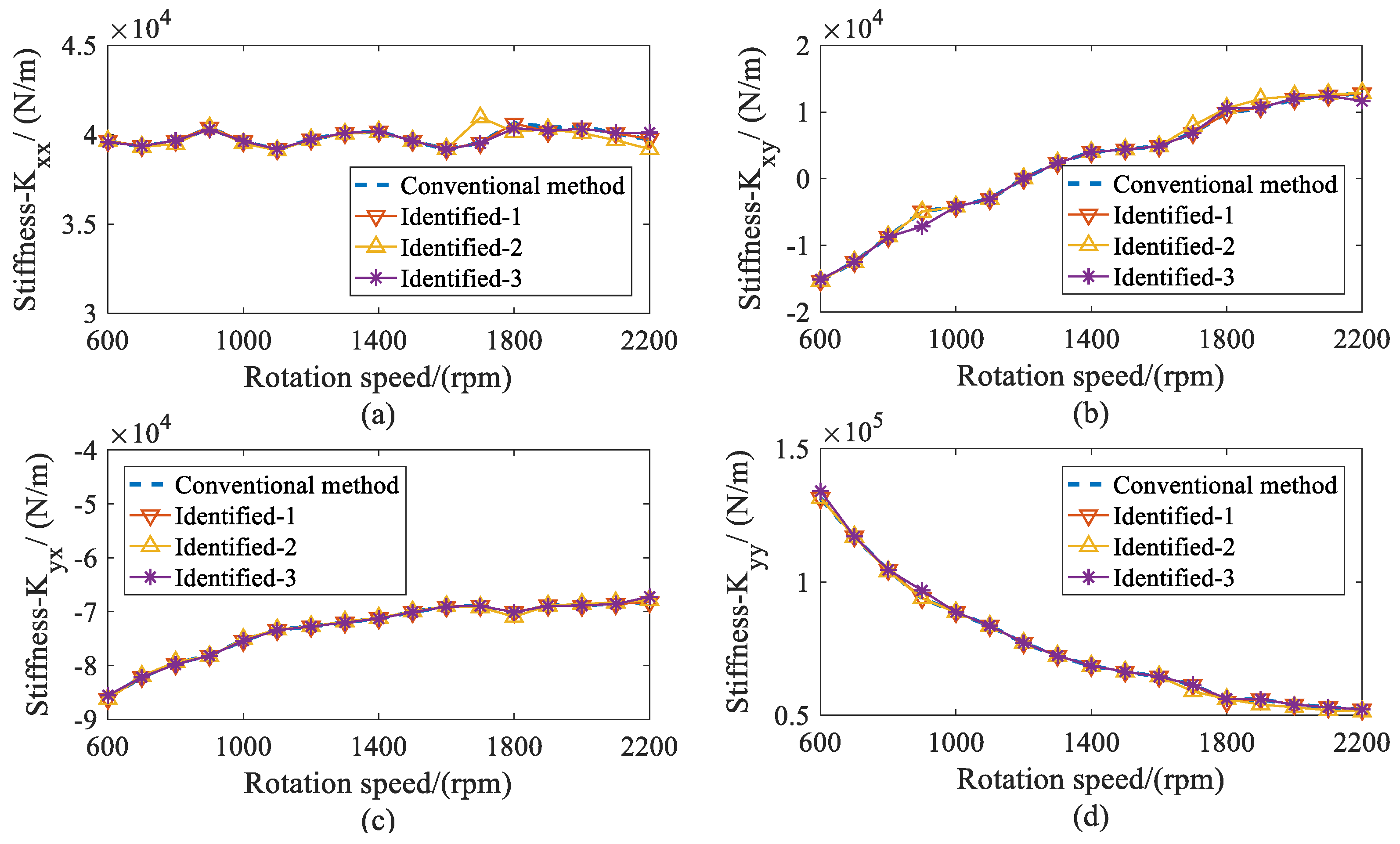
Figure 13.
Comparison for damping coefficients of bearing 1 versus rotor speed. (a) direct damping coefficients Cxx; (b) cross-coupled damping coefficients Cxy; (c) cross-coupled damping coefficients Cyx; (d) direct damping coefficients Cyy.
Figure 13.
Comparison for damping coefficients of bearing 1 versus rotor speed. (a) direct damping coefficients Cxx; (b) cross-coupled damping coefficients Cxy; (c) cross-coupled damping coefficients Cyx; (d) direct damping coefficients Cyy.
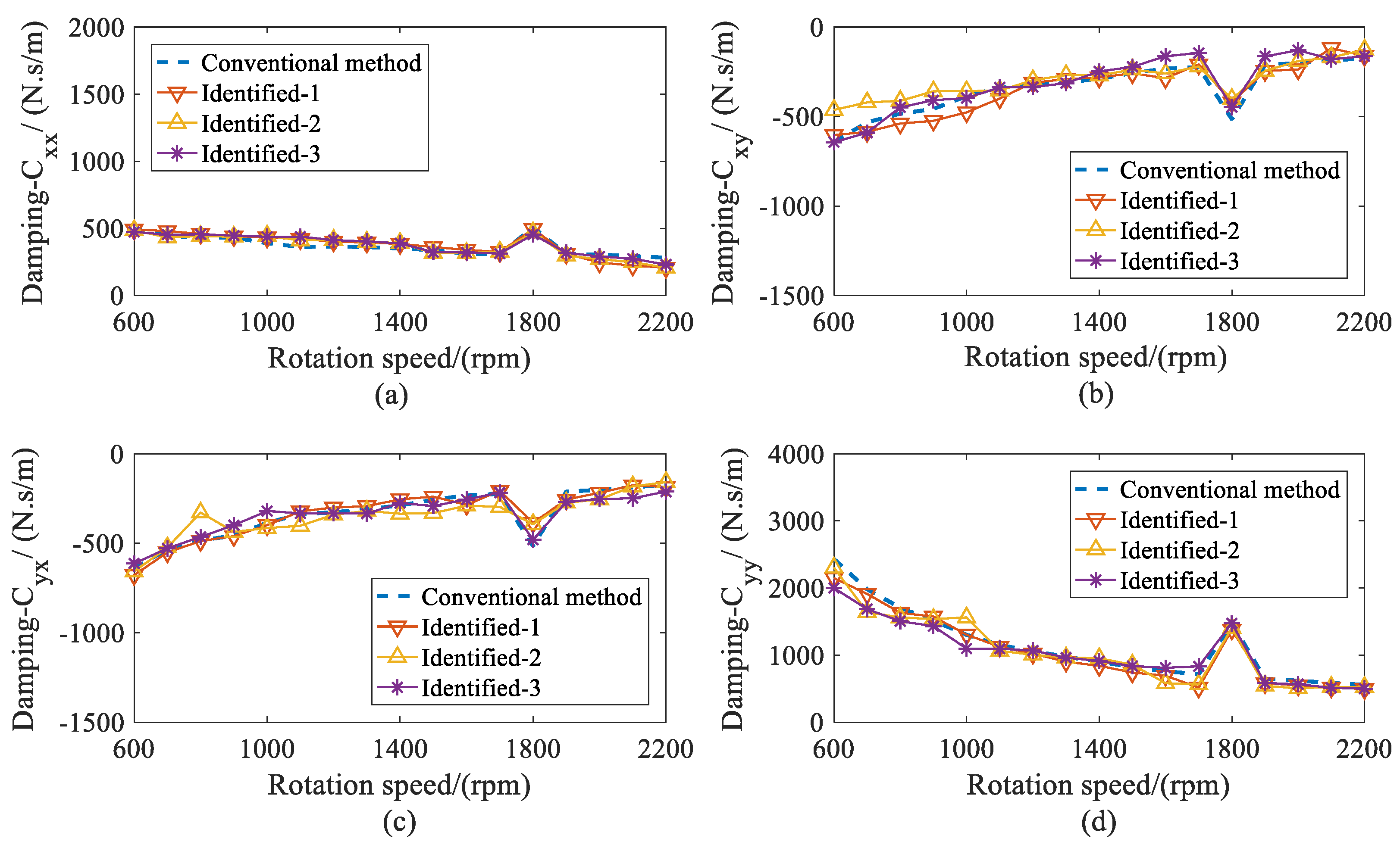
Figure 14.
Comparison for stiffness coefficients of bearing 2 versus rotation speed. (a) direct stiffness coefficient Kxx; (b) cross-coupled stiffness coefficient Kxy; (c) cross-coupled stiffness coefficients Kyx; (d) direct stiffness coefficients Kyy.
Figure 14.
Comparison for stiffness coefficients of bearing 2 versus rotation speed. (a) direct stiffness coefficient Kxx; (b) cross-coupled stiffness coefficient Kxy; (c) cross-coupled stiffness coefficients Kyx; (d) direct stiffness coefficients Kyy.
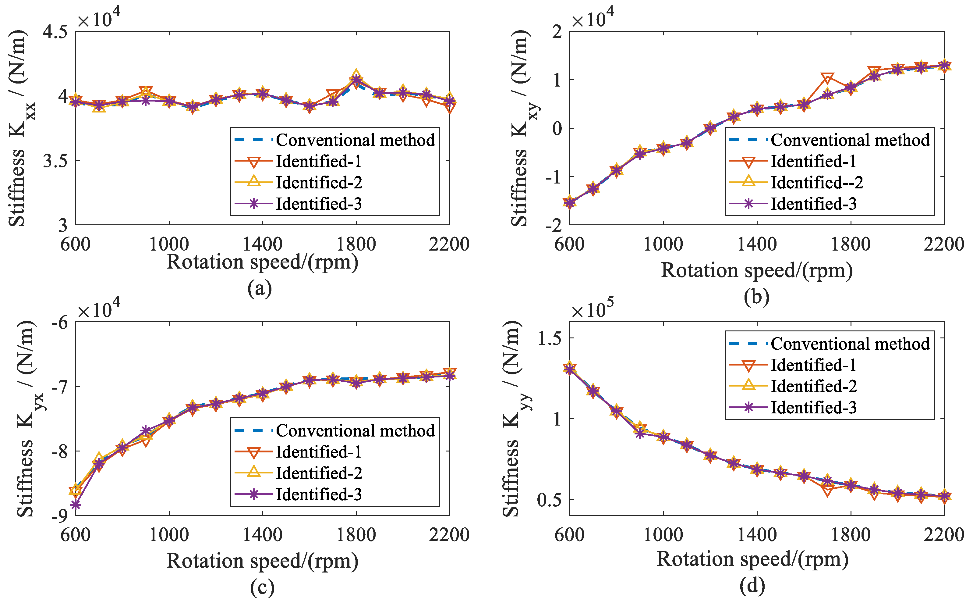
Figure 15.
Comparison for damping coefficients of bearing 2 versus rotor speed; (a) direct damping coefficients Cxx; (b) cross-coupled damping coefficients Cxy; (c) cross-coupled damping coefficients Cyx; (d) direct damping coefficients Cyy.
Figure 15.
Comparison for damping coefficients of bearing 2 versus rotor speed; (a) direct damping coefficients Cxx; (b) cross-coupled damping coefficients Cxy; (c) cross-coupled damping coefficients Cyx; (d) direct damping coefficients Cyy.
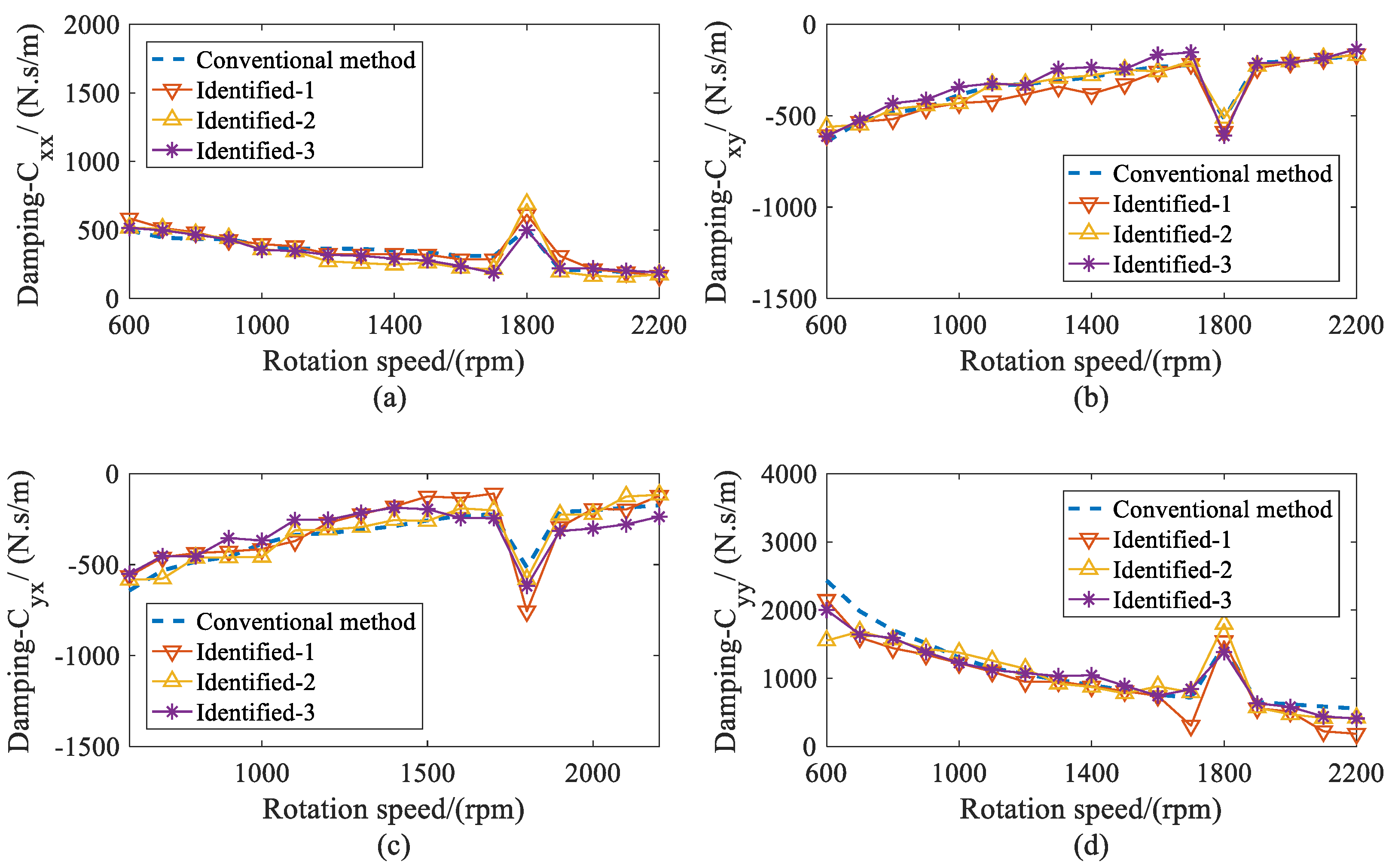
Figure 16.
Error between the proposed and conventional method. (a) stiffness coefficients of bearing 1; (b) damping coefficients of bearing 1; (c) stiffness coefficients of bearing 2; (d) damping coefficients of bearing 2.
Figure 16.
Error between the proposed and conventional method. (a) stiffness coefficients of bearing 1; (b) damping coefficients of bearing 1; (c) stiffness coefficients of bearing 2; (d) damping coefficients of bearing 2.

Table 1.
The parameters of the test rig.
| Property | Value |
|---|---|
| Rotor Shaft diameter, R | 0.01265 m |
| Maximum rotation speed, Ω | 6000 rpm |
| Mass, m | 0.86 kg |
| Length of rotor, L | 0.85 m |
| Density | 7800 kg/m3 |
| Rigid discs Inner diameter | 0.01265 m |
| Outer diameter | 0.08 m |
| Thickness | 0.015 m |
| Bearing Diameter | 0.01265 m |
| Length to diameter ratio | 1 |
| Radical clearance of bearings | 5 × 10⁻⁵ m |
Table 2.
Measured and theoretical (initial, updated) modal frequencies.
| Order | Initial Model (Hz) | Measured (Hz) | Updated Model (Hz) |
|---|---|---|---|
| 1 | 69.26 | 62.86 | 62.86 |
| 2 | 129.75 | 110.20 | 110.55 |
| 3 | 287.31 | 279.14 | 279.14 |
| 4 | 378.53 | 361.27 | 362.99 |
Table 3.
The parameters of the imbalance mass.
| Property | Mass (kg) | Radius (m) | Phase (°) |
|---|---|---|---|
| Node 8 | = 0.004 | r2 = 0.063 | 90 |
Table 4.
The parameters of the imbalance mass.
| Property | Mass (kg) | Radius (m) | Phase (°) |
|---|---|---|---|
| Node 4 | = 0.0025 | r1 = 0.063 | 0 |
| Node 8 | = 0.0050 | r2 = 0.063 | 90 |
© 2020 by the authors. Licensee MDPI, Basel, Switzerland. This article is an open access article distributed under the terms and conditions of the Creative Commons Attribution (CC BY) license (http://creativecommons.org/licenses/by/4.0/).
Share and Cite
MDPI and ACS Style
Kang, Y.; Shi, Z.; Zhang, H.; Zhen, D.; Gu, F. A Novel Method for the Dynamic Coefficients Identification of Journal Bearings Using Kalman Filter. Sensors 2020, 20, 565. https://doi.org/10.3390/s20020565
AMA Style
Kang Y, Shi Z, Zhang H, Zhen D, Gu F. A Novel Method for the Dynamic Coefficients Identification of Journal Bearings Using Kalman Filter. Sensors. 2020; 20(2):565. https://doi.org/10.3390/s20020565
Chicago/Turabian StyleKang, Yang, Zhanqun Shi, Hao Zhang, Dong Zhen, and Fengshou Gu. 2020. "A Novel Method for the Dynamic Coefficients Identification of Journal Bearings Using Kalman Filter" Sensors 20, no. 2: 565. https://doi.org/10.3390/s20020565
Note that from the first issue of 2016, this journal uses article numbers instead of page numbers. See further details here.