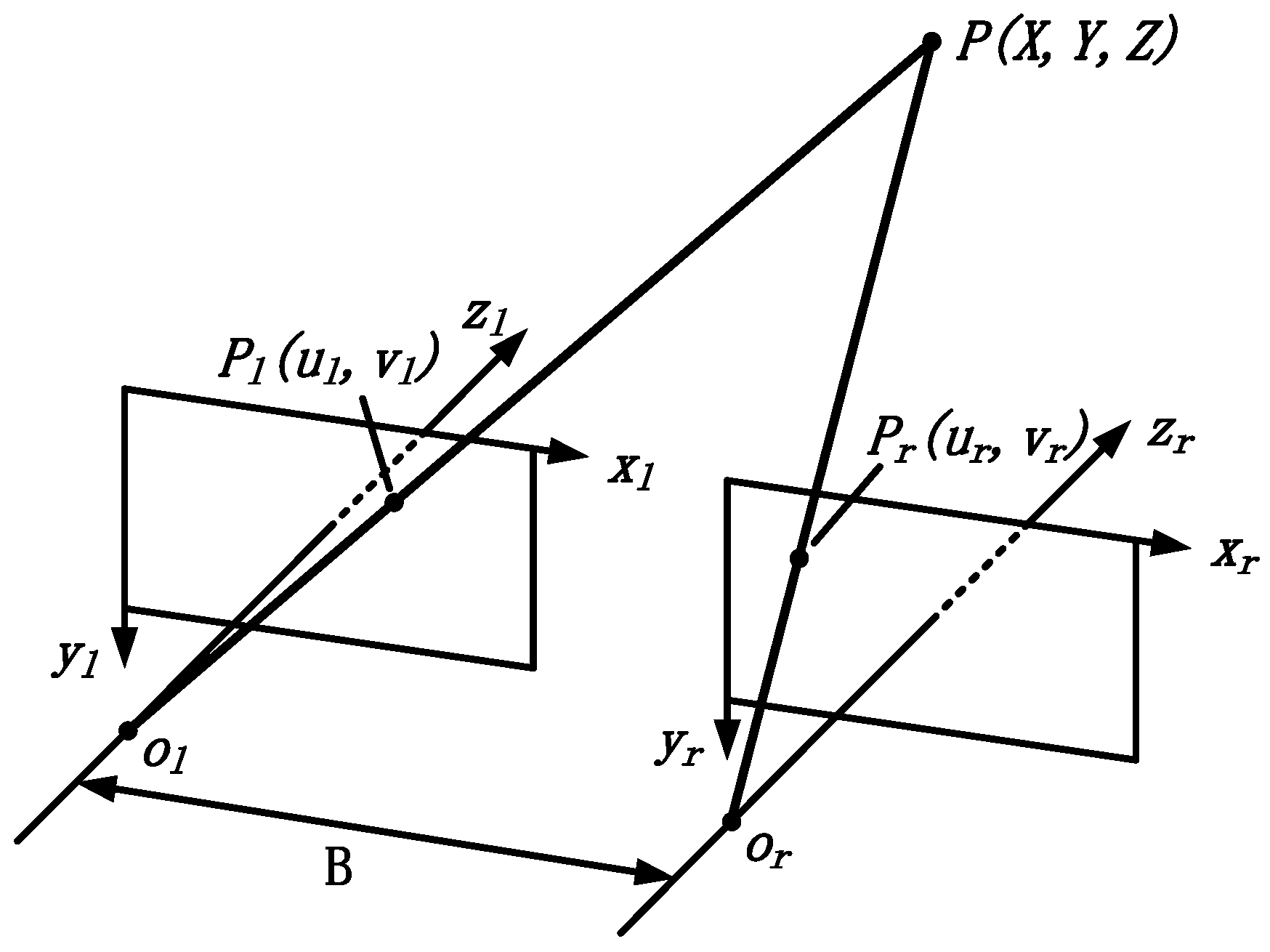
Stereo matching is one of the research focuses in computer vision, at its key ideal is to construct three-dimensional models for space scenes by matching the pixels in multiple images from different perspectives point-by-point and seeking for the three-dimensional coordinate of space points afterwards. Stereo matching is divided into four steps: cost initialization, cost aggregation, disparity computation and disparity optimization. And existing stereo matching algorithms can be categorized by global method and local method. The global method minimizes an energy function to obtain the optimal matching pixel while the local method overlays the pixel-value differencing of pixels in a local window. As the local method is advantageous in computation time and implementation, most of the stereo matching algorithms conduct similarity metric measuring based on pixels’ luminance or gray value, e.g., absolute intensity differences (AD), squared intensity differences (SD), adaptive weight, the Census transform [
16], etc. It is proved by Hirschmuller et al. that the method for acquiring matching cost based on the Census transform is robust to light distortion [
17]. Zhang et al. constructed a cross-based adaptive region based on the color differences of pixels [
18].
In terms of the advantages and disadvantages of current algorithms a stereo matching algorithm is proposed based on Gaussian-weighted AD-Census transform and improved cross-based adaptive regions; disparity optimization algorithm based on vote method, information entropy and region growing algorithm is adopted for the optimization of unreliable pixels’ disparities.
2.3.1. Cost Initialization
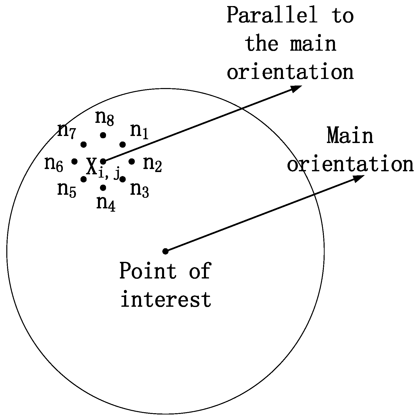
Traditional Census transformation (CT) compares gray value of a pixel with its neighborhood pixels’ gray value to generate a bit string, then the matching cost of two pixels is calculated by Hamming distance. For a pixel
p, the Census transformation is:
where
W(
p) is the neighborhood window of
p which has a gray value of
I(
p), and
q is pixels in
W(
p). CT only considers the gray relationship between
p and each of its neighborhood pixels and ignores the position relationship. Thus, the pixel value of
p is replaced by the Gaussian-weighted value in this paper, and the equation is:
where
Iwm is the weighted pixel value,
is the sum of weights,
x and
y is the position offset of the pixels in the window towards the center pixel
p, and
is a standard deviation of 1.5.
Assuming that
p(
x,
y) is a pixel in the left image,
q(
x − d,
y) is the correspondent pixel in the right image, and
d is the disparity of the two pixels. Taking two separate costs
Ccensus(
p,
d) and
CAD(
p,
d) into consideration,
CAD is the sum of the absolute values of color differences among
R,
G,
B components between the two pixels, and
Ccensus is defined as the Hamming distance of the Census strings of them:
Combine the two costs above, the total cost function is:
where
is a robust function on variable
:
2.3.2. Improved Cross-Based Local Support Region Construction
In stereo matching, the optimal matching pixels are retained by comparing the similarities between the reference pixel in the reference image and every waiting-for-matched pixel in the searching range of maximum disparity in another image. Meanwhile, it’s easy to occur mismatch because of the low distinctiveness of a single pixel. So, the window in an appropriate size for similarity matching should be created to improve the distinctiveness.
Utilizing the assumption that pixels with similar intensity within a constrained area are likely from the same image structure and have similar disparity, Zhang [
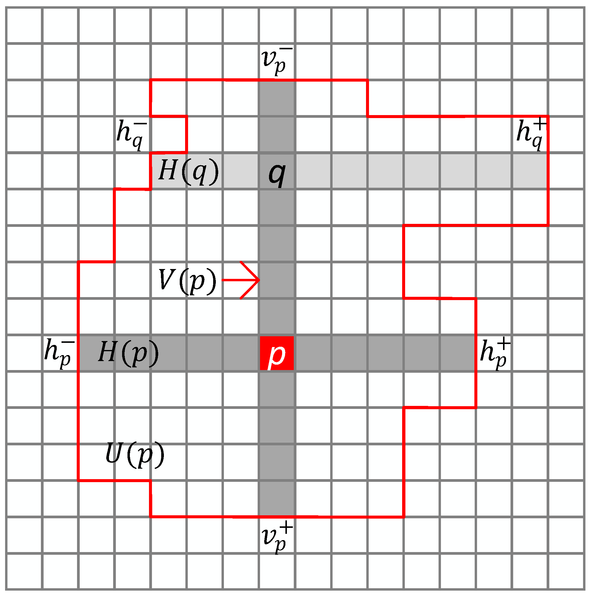
18] put forward a method for constructing a cross-base local support region for each pixel. For the anchor pixel
, construct a cross-based region composed by the horizontal segment
H(
p) and the vertical segment
V(
p) as the initial local support skeleton (see
Figure 5). The size of the cross-based region is determined by
which denotes the left, right, up, bottom arm length respectively. The determination criteria of the arm length are:
;
;
In criterion 1,
is defined as the maximum value of the color difference between
and
; in criterion 2,
is the space distance of the two pixels, which limits the maximum value of the arm length and avoids excessive growth of the local window.
and
L is the preset color and distance threshold. This method only takes into account the color differences between every regional pixel and the anchor pixel and is lack of consideration in the color differences of adjacent pixels. On this basis, the criterions are improved by increasing a gradient threshold for adjacent pixels and two different color thresholds in this paper. The gradient value is computed by Scharr operator [
19] here. The optimized criteria are:
;
;
;
where and are two different color thresholds (), and are two different distance thresholds (), and is a gradient threshold for adjacent pixels. For textureless areas, when the distance exceeds , a large window can be acquired while the excessive growth of the window is avoided by using the smaller threshold . For textured areas, the larger color gradient is used to retain the window in an appropriate size.
For edge and discontinuous areas, adjustments for thresholds are required to further reduce the growth of windows. Canny operator [
20] is used to filter out the edge and discontinuous areas as the white areas shown in
Figure 6. For these areas, the adjusting criteria are given here:
;
thresholds do not change, ;
The four arm lengths
for the pixel
can be confirmed by the improved criterion, and then the horizontal segment
H(
p) and the vertical segment
V(
p) can be acquired:
Zhang models the local support region by integrating multiple horizontal segments
H(
q), sliding along the vertical segment
V(
p) of the pixel
p, which only considers the differences among horizontal pixels and ignores the differences among vertical pixels. On this basis, the local region is constructed by jointing two windows, one of the windows is modeled by Zhang’s method and another is modeled by integrating multiple vertical segments
V(
q) sliding along the horizontal segment
H(
p) of the pixel
p:
2.3.4. Disparity Optimization
There are mismatches in the matching process, which lead to the deviation between the initial disparity and the real disparity. Therefore, the initial disparity reliability should be verified and the wrong disparity needs to be optimized.
Left-Right-Differences (LRD) is adopted to verify the initial disparity reliability and the specific method is implemented as follows: choose the left image as the reference image while the right one is the waiting-for-matched image to get one disparity map as
, and then reverse this process to get another disparity map as
. It is assumed that the disparity of the pixel
in
is
and the disparity of the pixel
in
is
. The initial disparity reliability of
can be verified by the formula:
where
is a preset threshold. If the difference between
and
is greater than
,
is considered to be invalid and its disparity is unreliable. Otherwise,
is considered to be valid and its disparity is reliable.
For every unreliable disparities, an optimization method based on region voting is proposed. Suppose is an invalid pixel. Then, count up number of all pixels as N and number of valid pixels as in the cross-based region of . And according to and N, there are three conditions for optimization:
Condition 1: If , search for the nearest valid pixel from to the left and right and replace the disparity of with the disparity of the valid pixel found. If no valid pixels are found, search to the top and bottom.
Condition 2: If , the average value of the disparities of all the valid pixels in the region is calculated as the optimized disparity of .
Condition 3: If , construct a disparity histogram and replace the disparity of with the value of the bin with the highest peak.
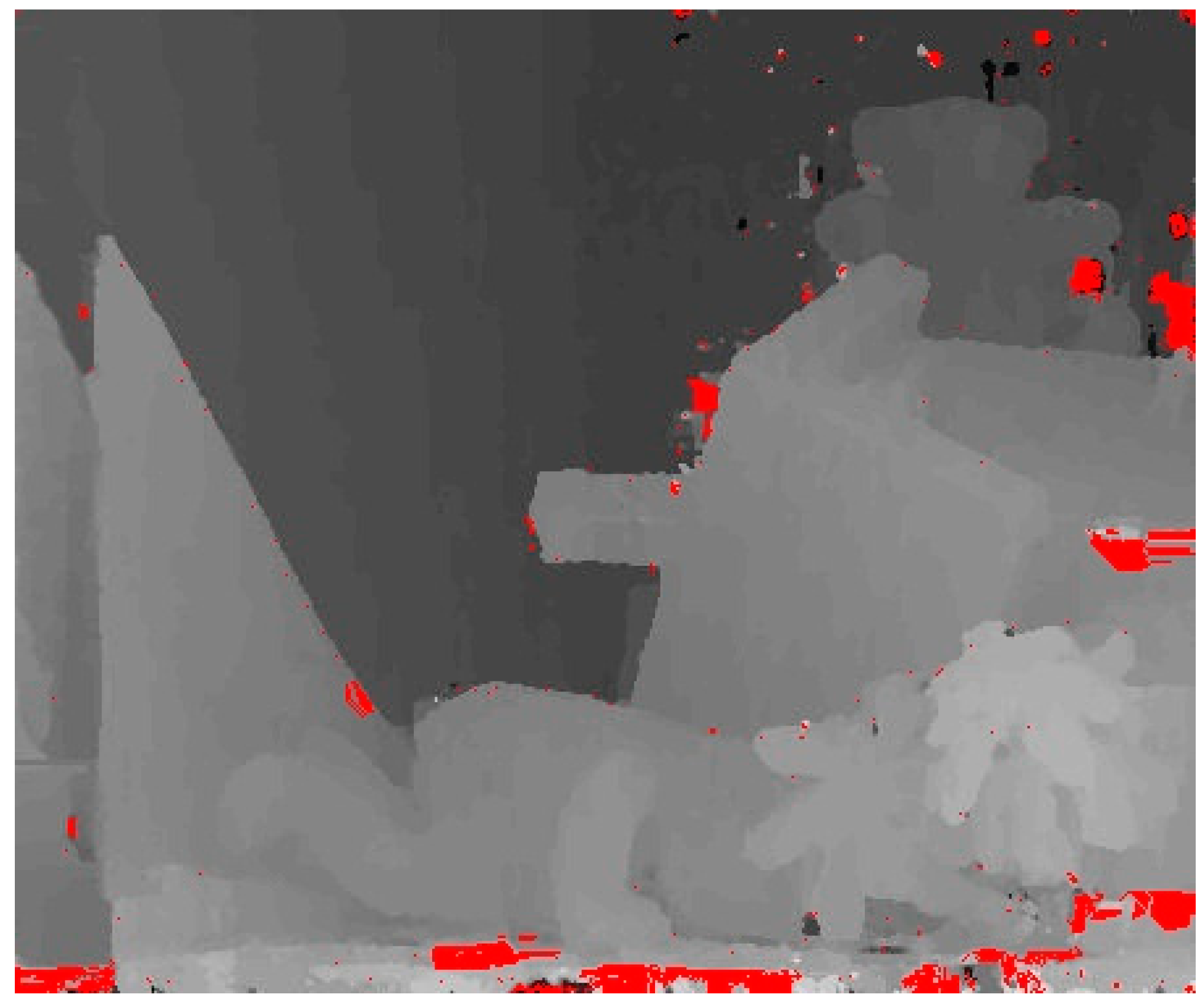
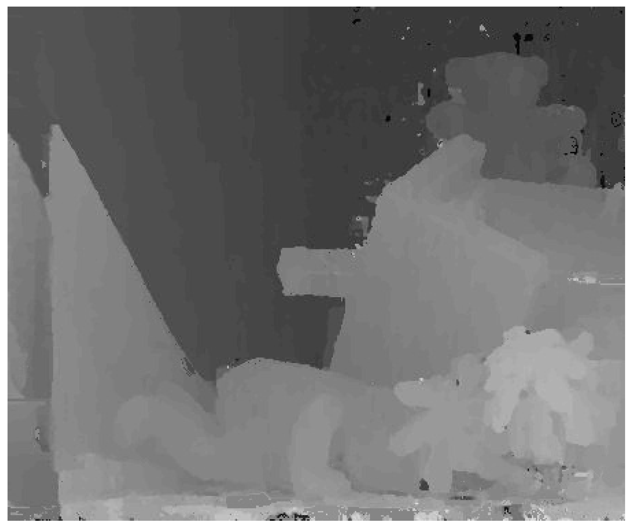
Finally, the optimized invalid pixels are set as valid pixels. The disparity optimization method can be performed on all invalid pixels effectively and most of disparities can be ensured to be reliable. Nevertheless, there may be mismatches caused by occlusion which result that the initial disparities deviated from the real disparities are considered to be reliable by LRD and can’t be optimized by the proposed disparity optimization method. For parts of the pixels with these disparities shown in
Figure 8 (the red areas), a method based on image entropy and region-growing algorithm is proposed to extract them and optimize their disparities.
Image entropy is a kind of information entropy which represents geometric average of the image grayscale and its magnitude shows the intensity of the change in pixels [
21]. The calculation equation of one-dimensional image entropy is as follows:
where
represents the appearance probabilities of gray value in a local window. Set the pixels whose entropy is less than 0.5 as invalid pixels and expend the regions around these pixels by region-growing algorithm. The algorithm is as follows:
Step 1: Choose one pixel from the invalid pixels as an initial pixel each time.
Step 2: Search the neighborhood pixels of . If and hasn’t been searched, set as another initial pixel.
Step 3: Repeat the Step 2 until all the initial pixels has been searched, then a consecutive region is obtained. If the number of the pixels in the region is smaller than 2000, set all the pixels in the region as invalid pixels. Otherwise, set them as valid pixels.
Step 4: Repeat Step 1 until all the invalid pixels has been chosen.
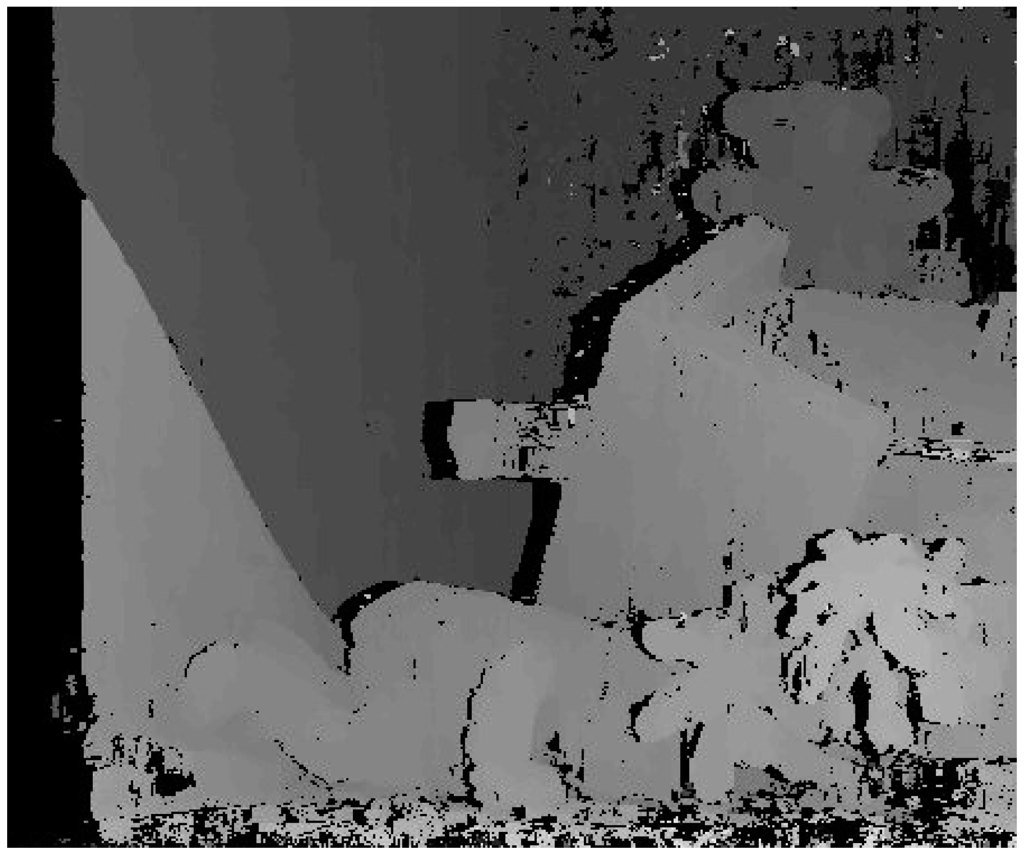
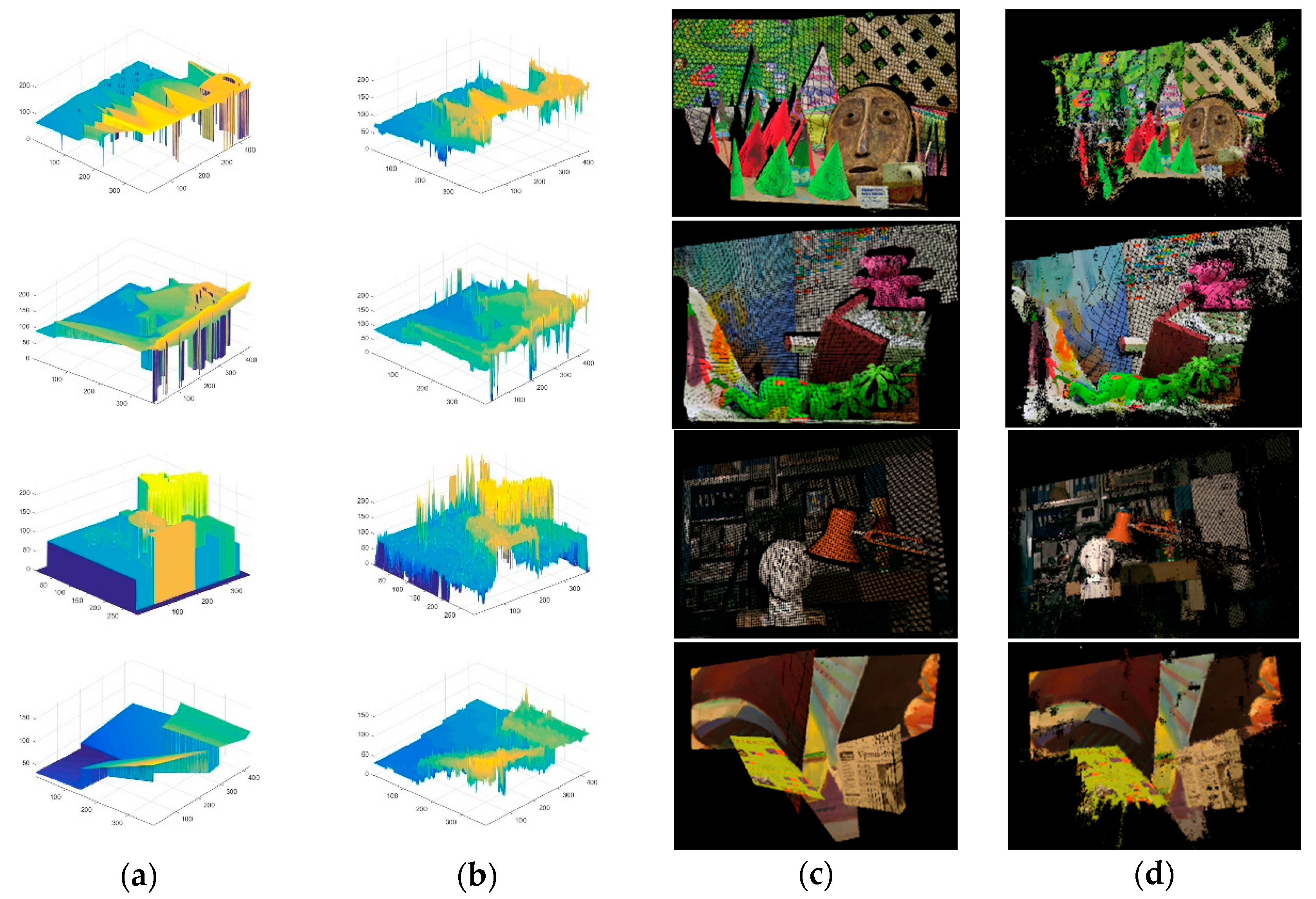
For the invalid pixels obtained by region-growing algorithm, the proposed disparity optimization method is adopted to optimize their disparities. As shown in
Figure 9, disparities of most of mismatched pixels are effectively optimized.


