Accurate Calibration of Multi-LiDAR-Multi-Camera Systems


Abstract
:1. Introduction
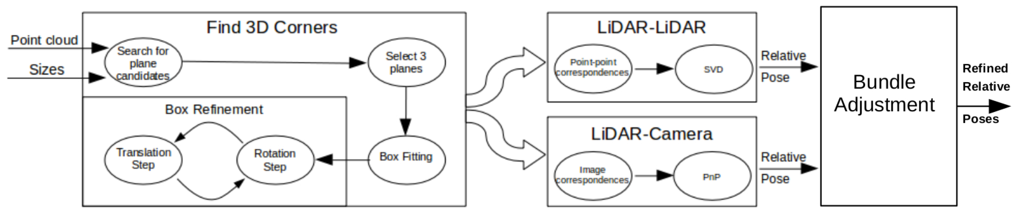
2. Calibration Outline
- Camera-LiDAR calibration: Projections of the box corners need to be selected in the camera image. The spatial (LiDAR) and 2D (camera) point correspondences define a PnP problem, which can be effectively solved by, e.g., the EPnP algorithm [16].
- LiDAR-LiDAR calibration: The corners of the same calibration box need to be calculated in the two point clouds, separately. Then, the extrinsic parameters can be found by point registration.
- Car Body-LiDAR calibration: The last calibration step is to estimate the car body location with respect to the sensors. This step is independent of the camera-LiDAR and LiDAR-LiDAR calibrations. A single plane is required that can be placed at four different locations: to the left and right side, in front of and behind the car. This step is essential for autonomous driving, as car dimension determines the free space of the car in order to avoid collision.
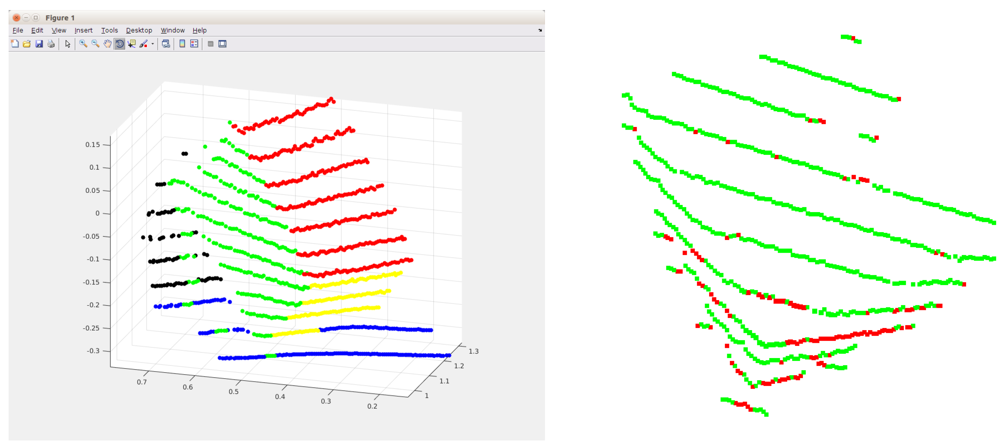
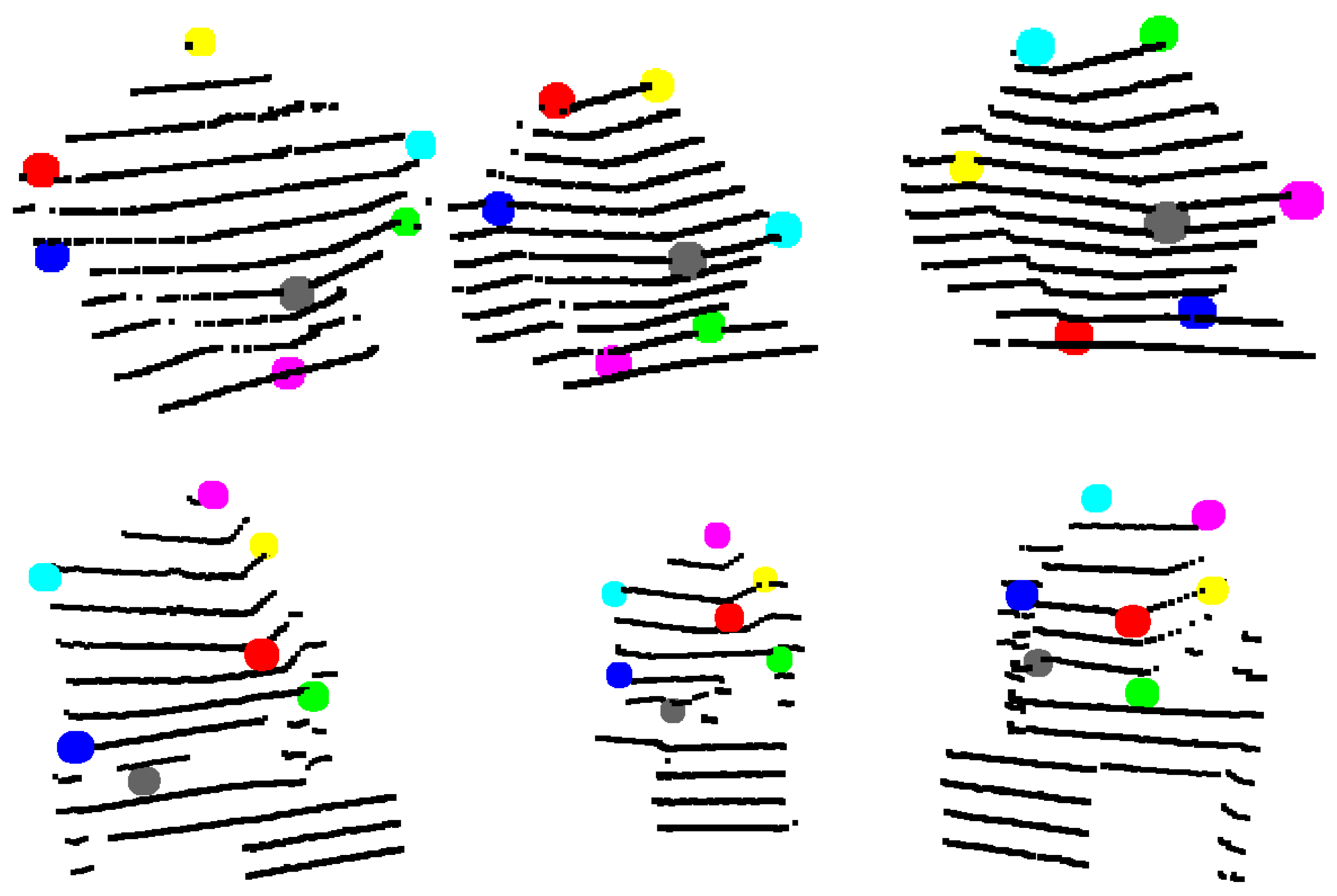
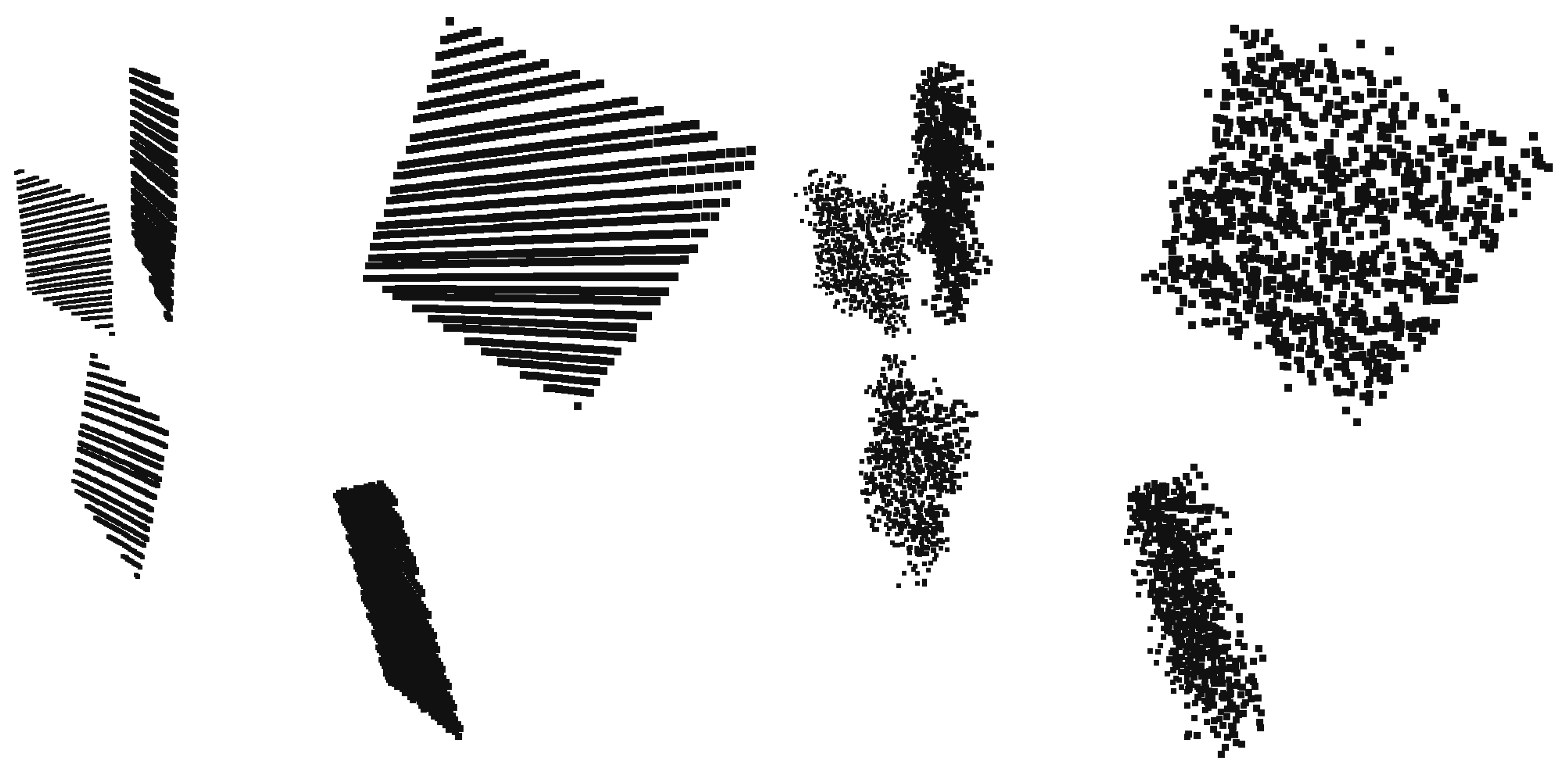
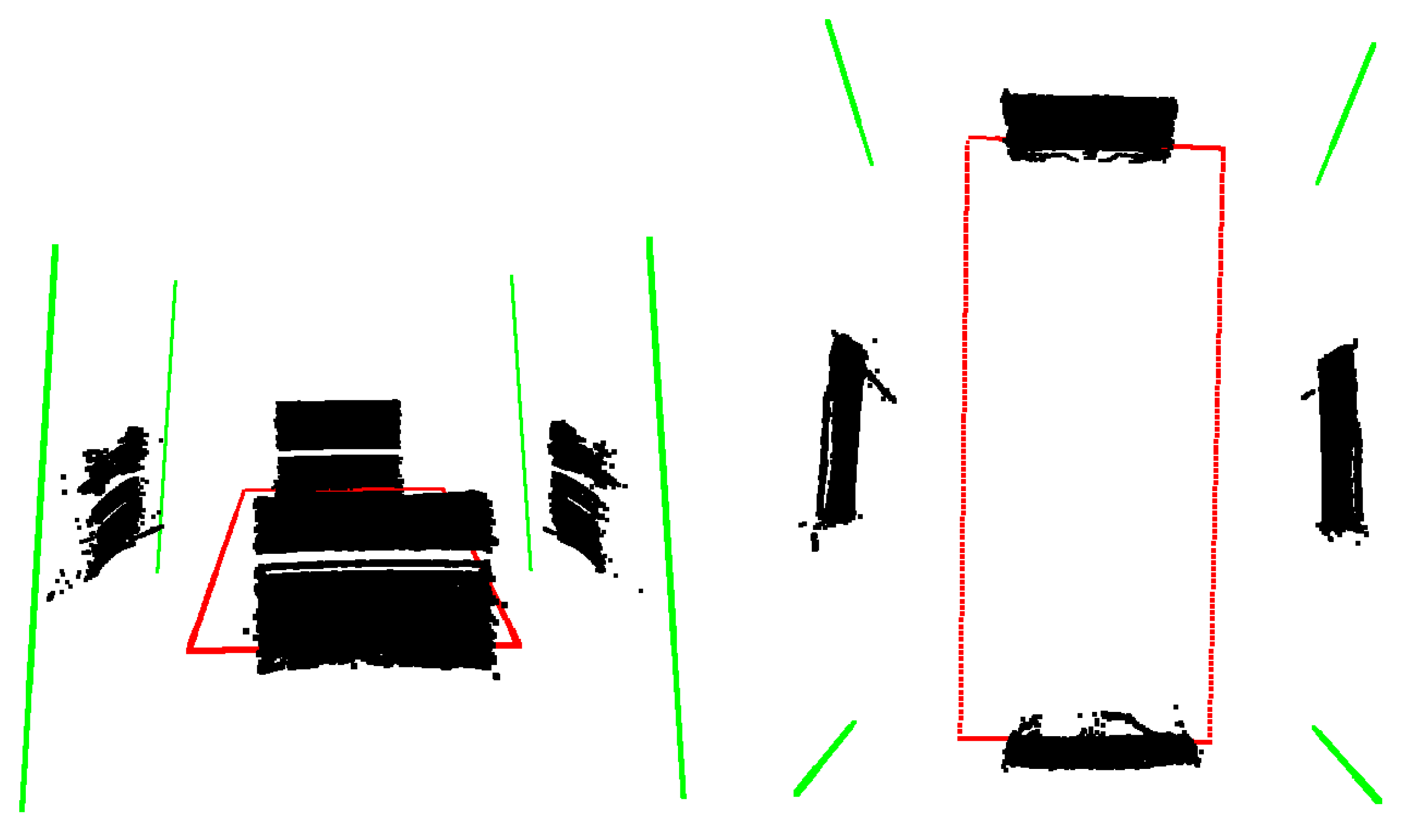
3. Estimation of Box Corners in the LiDAR Point Cloud
3.1. Finding the Planes of the Box
3.2. Outlier Filtering
3.3. Iterative Box Refinement
3.3.1. Rotation Step
3.3.2. Translation Step
3.4. Convergence
4. Getting the Extrinsic Parameters
4.1. LiDAR-Camera Calibration
4.2. LiDAR-LiDAR Calibration
5. LiDAR-Camera System Calibration
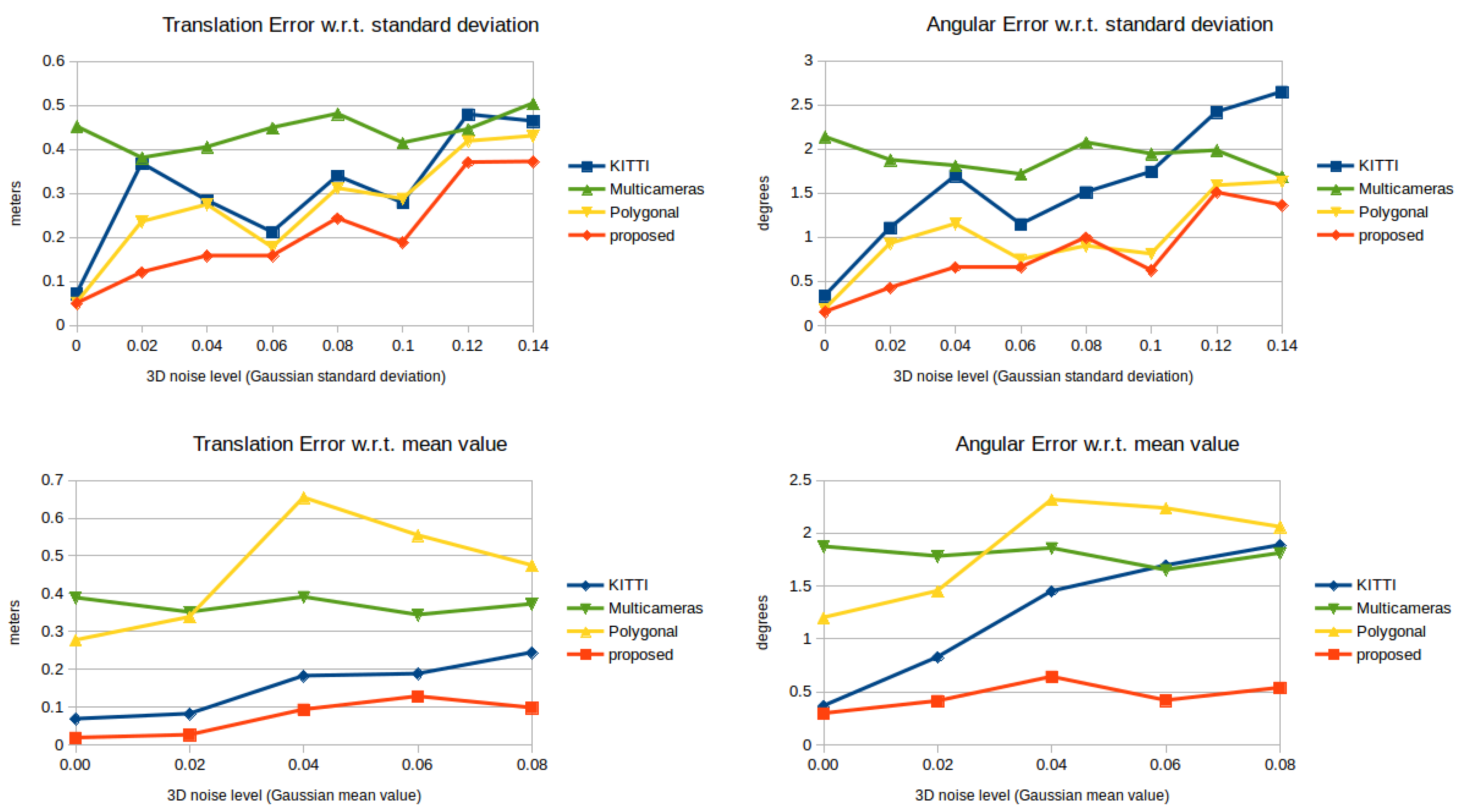
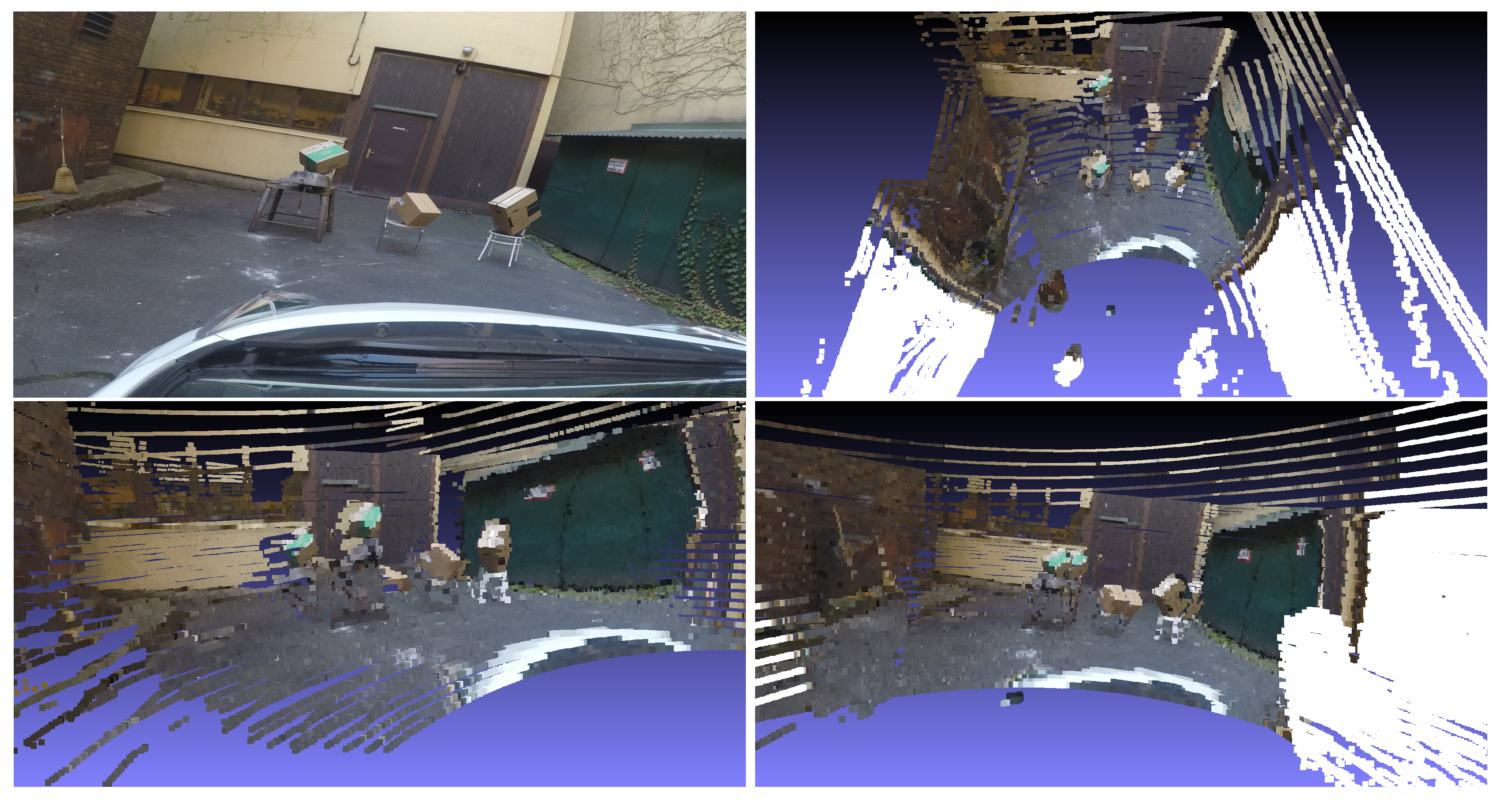
6. Tests
6.1. Synthetic Tests
- the KITTI calibration toolbox (denoted as KITTI),
- the calibration method by Park et al. (denoted as polygonal),
- the automatic calibration by Hassanein et al. (denoted as multi-camera),
- and the proposed method (denoted as proposed).
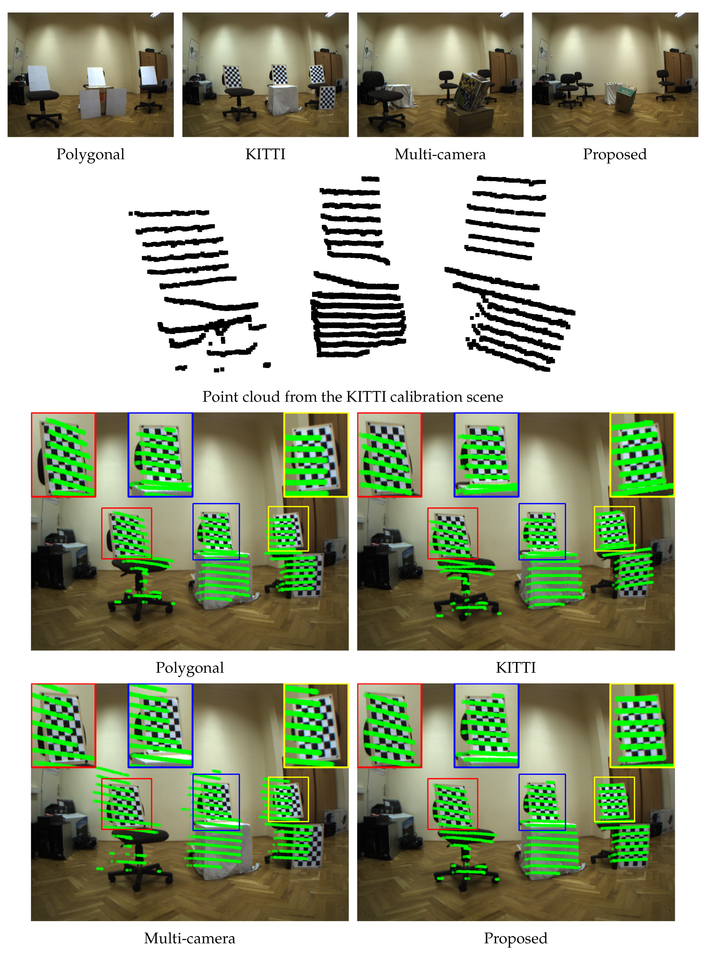
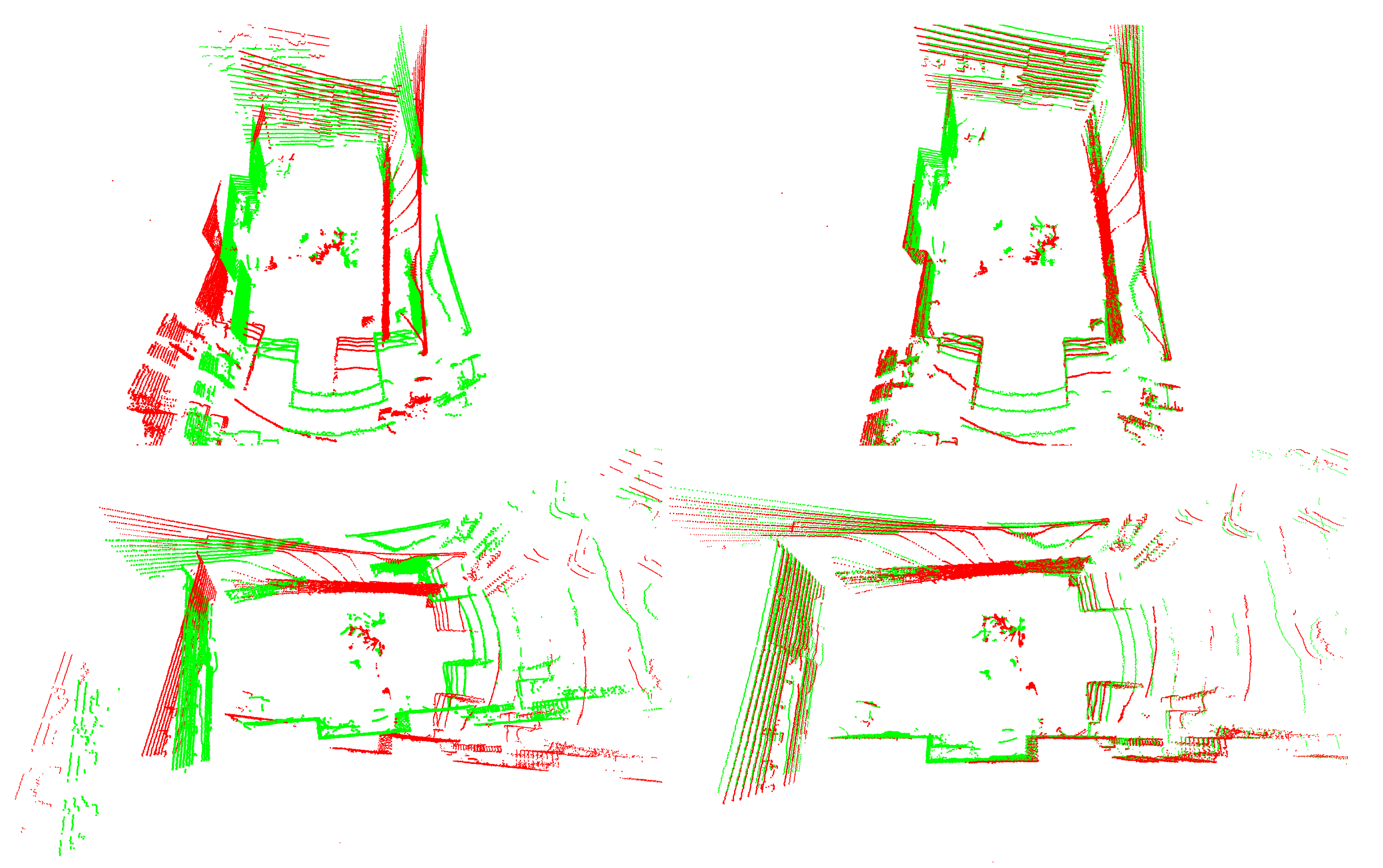
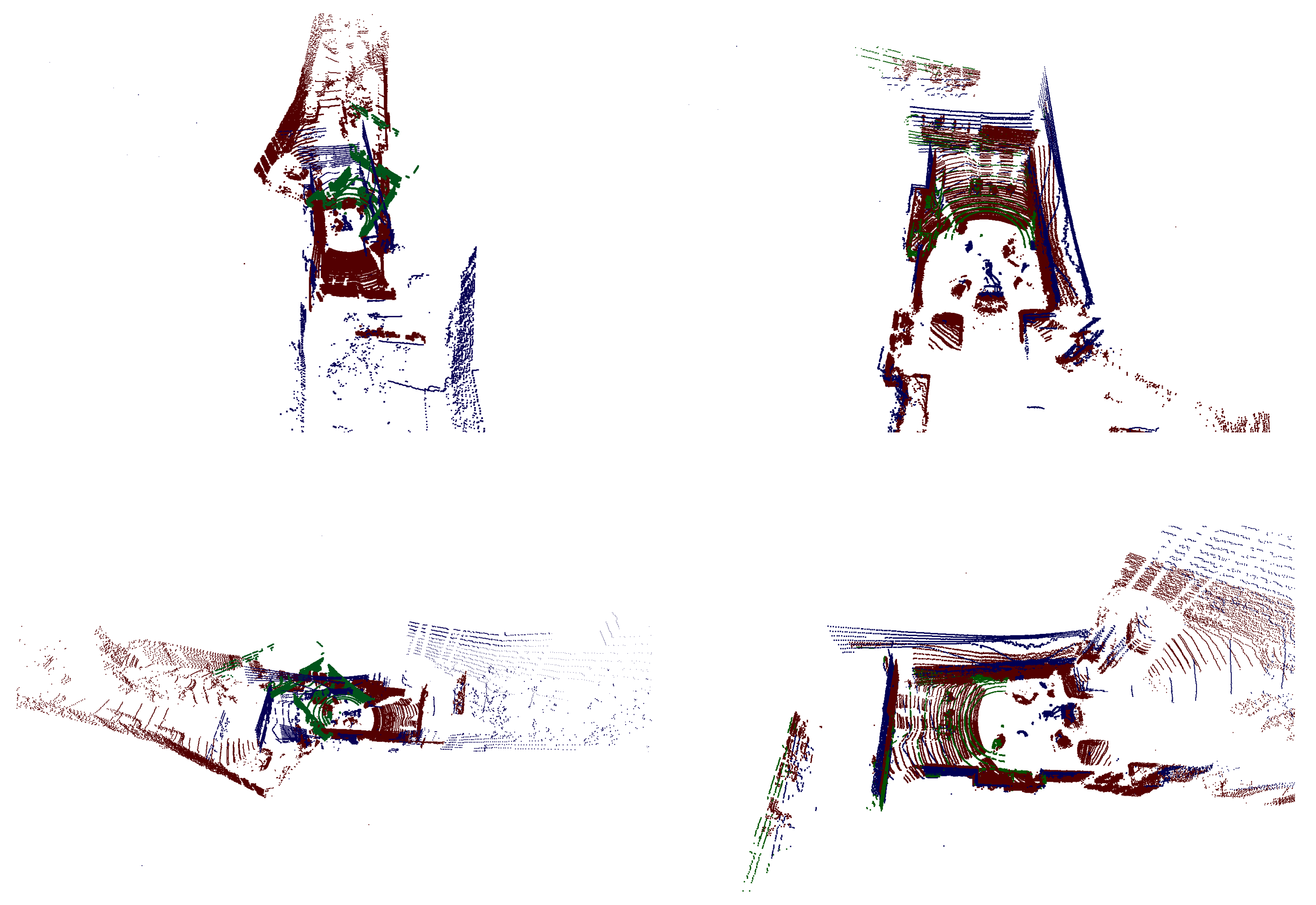
6.2. Real-World Tests
7. Calibration of Car Dimensions
8. Conclusions
Author Contributions
Funding
Conflicts of Interest
Appendix A. Convergence of Iterative Box Fitting
References
- Fremont, V.; Bonnifait, P. Extrinsic calibration between a multi-layer lidar and a camera. In Proceedings of the 2008 IEEE International Conference on Multisensor Fusion and Integration for Intelligent Systems, Seoul, Korea, 20–22 August 2008; pp. 214–219. [Google Scholar]
- Levenberg, K. A method for the solution of certain problems in least squares. Q. Appl. Math. 1944, 2, 164–168. [Google Scholar] [CrossRef]
- Marquardt, D. An algorithm for least-squares estimation of nonlinear parameters. SIAM J. Appl. Math. 1963, 11, 431–441. [Google Scholar] [CrossRef]
- Alismail, H.; Baker, L.D.; Browning, B. Automatic calibration of a range sensor and camera system. In Proceedings of the 2012 Second International Conference on 3D Imaging, Modeling, Processing, Visualization & Transmission, Zurich, Switzerland, 13–15 October 2012; pp. 286–292. [Google Scholar]
- Fischler, M.A.; Bolles, R.C. Random Sample Consensus: A Paradigm for Model Fitting with Applications to Image Analysis and Automated Cartography. Commun. ACM 1981, 24, 381–395. [Google Scholar] [CrossRef]
- Chen, Y.; Medioni, G. Object Modelling by Registration of Multiple Range Images. Image Vis. Comput. 1992, 10, 145–155. [Google Scholar] [CrossRef]
- Park, Y.; Yun, S.; Won, C.S.; Cho, K.; Um, K.; Sim, S. Calibration between color camera and 3D LIDAR instruments with a polygonal planar board. Sensors 2014, 14, 5333–5353. [Google Scholar] [CrossRef] [PubMed]
- Gong, X.; Lin, Y.; Liu, J. 3D LIDAR-Camera Extrinsic Calibration Using an Arbitrary Trihedron. Sensors 2013, 13, 1902–1918. [Google Scholar] [CrossRef] [PubMed] [Green Version]
- Veĺas, M.; Španěl, M.; Materna, Z.; Herout, A. Calibration of RGB Camera With Velodyne LiDAR. In WSCG 2014 Communication Papers Proceedings; Union Agency: Plzen, Czech Republic, 2014; Volume 2014, pp. 135–144. [Google Scholar]
- Levinson, J.; Thrun, S. Automatic Online Calibration of Cameras and Lasers. In Proceedings of the Robotics: Science and Systems, Berlin, Germany, 24–28 June 2013. [Google Scholar]
- Geiger, A.; Moosmann, F.; Car, O.; Schuster, B. Automatic camera and range sensor calibration using a single shot. In Proceedings of the 2012 IEEE International Conference on Robotics and Automation (ICRA), St. Paul, MN, USA, 14–18 May 2012; pp. 3936–3943. [Google Scholar]
- Hassanein, M.; Moussa, A.; El-Sheimy, N. A new automatic system calibration of multi-cameras and lidar sensors. ISPRS Int. Arch. Photogramm. Remote Sens. Spat. Inf. Sci. 2016, 41, 589–594. [Google Scholar] [CrossRef]
- Bay, H.; Ess, A.; Tuytelaars, T.; Van Gool, L. Speeded-Up Robust Features (SURF). Comput. Vis. Image Underst. 2008, 110, 346–359. [Google Scholar] [CrossRef] [Green Version]
- Besl, P.J.; McKay, N.D. A Method for Registration of 3-D Shapes. IEEE Trans. Pattern Anal. Mach. Intell. 1992, 14, 239–256. [Google Scholar] [CrossRef]
- Pusztai, Z.; Hajder, L. Accurate Calibration of LiDAR-Camera Systems Using Ordinary Boxes. In Proceedings of the 2017 IEEE International Conference on Computer Vision Workshops, Venice, Italy, 22–29 October 2017; pp. 394–402. [Google Scholar]
- Lepetit, V.; Moreno-Noguer, F.; Fua, P. EPnP: An Accurate O(n) Solution to the PnP Problem. Int. J. Comput. Vis. 2009, 81, 155. [Google Scholar] [CrossRef] [Green Version]
- Zheng, Y.; Kuang, Y.; Sugimoto, S.; Åström, K.; Okutomi, M. Revisiting the PnP Problem: A Fast, General and Optimal Solution. In Proceedings of the 2013 IEEE International Conference on Computer Vision, Sydney, Australia, 1–8 December 2013; pp. 2344–2351. [Google Scholar]
- Pandey, G.; McBride, J.R.; Savarese, S.; Eustice, R.M. Automatic Extrinsic Calibration of Vision and LiDAR by Maximizing Mutual Information. J. Field Robot. 2015, 32, 696–722. [Google Scholar] [CrossRef]
- Wang, W.; Sakurada, K.; Kawaguchi, N. Reflectance Intensity Assisted Automatic and Accurate Extrinsic Calibration of 3D LiDAR and Panoramic Camera Using a Printed Chessboard. Remote Sens. 2017, 9, 851. [Google Scholar] [CrossRef]
- Isack, H.; Boykov, Y. Energy-Based Geometric Multi-model Fitting. Int. J. Comput. Vis. 2012, 97, 123–147. [Google Scholar] [CrossRef]
- Pham, T.; Chin, T.; Schindler, K.; Suter, D. Interacting Geometric Priors For Robust Multimodel Fitting. IEEE Trans. Image Process. 2014, 23, 4601–4610. [Google Scholar] [CrossRef] [PubMed]
- Toldo, R.; Fusiello, A. Robust Multiple Structures Estimation with J-Linkage. In Computer Vision—ECCV 2008; Forsyth, D., Torr, P., Zisserman, A., Eds.; Springer: Berlin/Heidelberg, Germany, 2008; pp. 537–547. [Google Scholar]
- Harris, C.; Stephens, M. A combined corner and edge detector. In Proceedings of the Fourth Alvey Vision Conference, Manchester, UK, 31 August–2 September 1988; pp. 147–151. [Google Scholar]
- Triggs, B.; McLauchlan, P.F.; Hartley, R.I.; Fitzgibbon, A.W. Bundle Adjustment—A Modern Synthesis. In Vision Algorithms: Theory and Practice; Triggs, W., Zisserman, A., Szeliski, R., Eds.; Springer: Berlin, Germany, 2000; Volume LNCS 1883, pp. 298–375. [Google Scholar]
- Blender Sensor Simulation. Available online: http://www.blensor.org (accessed on 1 July 2018).
- Rosten, E.; Drummond, T. Fusing Points and Lines for High Performance Tracking. In Proceedings of the Internation Conference on Computer Vision, Beijing, China, 17–21 October 2005; pp. 1508–1515. [Google Scholar]
- Eberly, D. Rotation Representations and Performance Issues; Magic Software, Inc.: Chapel Hill, NC, USA, 2002. [Google Scholar]
- Zhang, Z. A flexible new technique for camera calibration. IEEE Trans. Pattern Anal. Mach. Intell. 2000, 22, 1330–1334. [Google Scholar] [CrossRef] [Green Version]


| Automatic | # of Observations | Calibration Object | Strength | Weakness | |
|---|---|---|---|---|---|
| Rodrigues et al. [1] | no | 6 | planar with circular hole | low noise ratio by texture | no guarantee for convergence |
| Alismail et al. [4] | yes | 1 | black planar circle | automatic | the center of the circle must be marked |
| Park et al. [7] | no | 3 | white homogeneous, planar | no additional LiDAR noise by texture | estimated board edges |
| Gong et al. [8] | no | 2 | arbitrary trihedron | orthogonality of the object is not required | much human intervention |
| Velas et al. [9] | yes | 1 | planar with holes, white background | automatic | difficult calibration setup |
| Geiger et al. [11] | yes | 1 | planar, chessboards | only one shot is needed by sensors | multiple chessboards are needed |
| Hassanein et al. [12] | yes | 1 | well-textured trihedron | automatic | camera system must be pre-calibrated |
| Before BA | After BA | |||
|---|---|---|---|---|
| Camera | LiDAR | Camera | LiDAR | |
| Synthetic | 4.231 px | 0.02231 m | 2.152 px | 0.02001 m |
| Real-world | 2.892 px | 0.03515 m | 0.963 px | 0.01036 m |
| Method | 3D Scene | Camera | LiDAR |
|---|---|---|---|
| KITTI |  |  |  |
| Polygonal |  |  |  |
| Multi-camera |  |  |  |
| Proposed |  |  |  |
© 2018 by the authors. Licensee MDPI, Basel, Switzerland. This article is an open access article distributed under the terms and conditions of the Creative Commons Attribution (CC BY) license (http://creativecommons.org/licenses/by/4.0/).
Share and Cite
Pusztai, Z.; Eichhardt, I.; Hajder, L. Accurate Calibration of Multi-LiDAR-Multi-Camera Systems. Sensors 2018, 18, 2139. https://doi.org/10.3390/s18072139
Pusztai Z, Eichhardt I, Hajder L. Accurate Calibration of Multi-LiDAR-Multi-Camera Systems. Sensors. 2018; 18(7):2139. https://doi.org/10.3390/s18072139
Chicago/Turabian StylePusztai, Zoltán, Iván Eichhardt, and Levente Hajder. 2018. "Accurate Calibration of Multi-LiDAR-Multi-Camera Systems" Sensors 18, no. 7: 2139. https://doi.org/10.3390/s18072139
APA StylePusztai, Z., Eichhardt, I., & Hajder, L. (2018). Accurate Calibration of Multi-LiDAR-Multi-Camera Systems. Sensors, 18(7), 2139. https://doi.org/10.3390/s18072139