4.1. Correlative Responses
As an example,
Figure 4 shows the experiment results associated with potassium ferricyanide. Throughout the experiment, potassium ferricyanide solutions with concentrations of 1.0 mg L
−1, 2.0 mg L
−1, 4.0 mg L
−1, and 8.0 mg L
−1 were tested in turn. The concentrations are at the sensors, and are not the initial injected contaminant concentration via the peristaltic pump. This condition is indicated by solid green bars at the top of
Figure 4. In the figure, COD, NO
3-N, TOC, and residual chlorine increase because of the presence of potassium ferricyanide. In addition, the response of residual chlorine is relatively slow but stable; however, random fluctuations still occur in the stable state of the other three indicators. When the concentration of potassium ferricyanide at the sensors is greater than 1.0 mg/L, the numerical value of NH
3-N relative to the background also has an obvious upward trend. However, when the contaminant concentration is 1.0 mg/L or 0.5 mg/L or even less, the numerical value of the NH
3-N is irregular, which shows the easily variable characteristic of water quality parameters. Sensor responses show correlative relationships, especially for COD, NO
3-N, TOC, and residual chlorine, as well as reflect the response degree because of the induction of different contaminant concentrations.
Obviously, the response amplitudes of sensors are related to the contaminant concentrations. This fact suggests that correlative response and response amplitude are caused by the introduction of different contaminant concentrations and implies that this type of phenomenon can be utilized for quantitative evaluation of contaminants. In order to justify the feasibility and applicability of the proposed method, offline experiments of potassium ferricyanide were conducted before online potassium ferricyanide injection experiments. Although types and detection methods of water quality sensors used in offline experiments are different from those of online ones, the correlative responses of pH, conductivity, residual chlorine, total chlorine, and NH3-N are also presented in the offline experiments of potassium ferricyanide. The responses of sensors are similar to the case of online experiments, which indicates that the proposed approach can also be utilized for quantitative evaluation in offline cases. By comparing with results from other types of contaminants, the response curves are clearly contaminant-specific. Obviously, obtaining parameters that will change with the contaminant concentration is necessary, while the others are disposed of. In other words, sensitive parameter extraction is needed to determine the input parameters of the regression model.
4.2. Sensitive Parameter Extraction
Because the detection upper bound of NO
3-N is 2.0 mg/L, the maximum concentration of potassium ferricyanide in the training set is 18 mg/L. In
Figure 4, with the change in contaminant concentration, the change values relative to the baseline values of the water quality sensors are different. The change values of water quality parameters can be considered as the result of contaminant introduction and can be used for the quantitative analysis of contaminant concentration. The concept of relative response value was introduced to calculate the differences between water quality parameters and their baselines. Ideally, the maximum response value should be stable and completely caused by contaminant introduction, and not the superposition caused by water quality noise. For example, after the introduction of 1 mg/L and 8 mg/L potassium ferricyanide, significant single-point mutation noises appear in the TOC response data (
Figure 4). The maximum response value of NO
3-N occurs at the end of the response time, while no ideal stationary change appears in the response values of COD and NH
3-N.
Table 3 presents the relative response values of eight water quality parameters caused by potassium ferricyanide introductions with different concentrations. Other data processing methods for baseline values of water quality sensors are discussed in a later part of this paper.
The Pearson correlation coefficients for each sensor with potassium ferricyanide concentrations are calculated (
Table 3). In the table, the calculated Pearson correlation coefficients are 0.0746 (conductivity), 0.0886 (turbidity), 0.0533 (DO), 0.3748 (COD), 0.6080 (TOC), 0.7690 (NH
3-N), 0.7541 (NO
3-N), and 0.9997 (residual chlorine). In the regression model process of potassium ferricyanide, COD, TOC, NH
3-N, NO
3-N, and residual chlorine are chosen as the model inputs according to the description in
Section 2.2.3.
Figure 5 presents that the relative response values of TOC, NH
3-N, NO
3-N, and residual chlorine change with the concentration of potassium ferricyanide. The values of the abscissa represent the labels of experiments, and the left values of ordinate represent the concentrations values of potassium ferricyanide while the right values of ordinate represent the change values of TOC, NH
3-N, NO
3-N, and residual chlorine.
In the figure, a correlation exists between TOC and potassium ferricyanide. However, the Pearson correlation coefficient is relatively small because of the noise introduced by the seventh sample; and the relative response value of TOC in subsequent samples tend to saturate. The good linear correlation between residual chlorine and potassium ferricyanide concentration largely depends on the detection method for residual chlorine. Residual chlorine is measured once every 2.5 min but recorded every minute. It can be seen from the figure that the strength of the correlation between different water quality indicators and contaminant concentrations is different, and the reason for this difference is that there is a local nonlinearity in the relative response.
4.3. Modeling and Test
A simple method for model selection is to randomly divide the data set into three parts, namely training set, validation set, and test set. The training set is used to train the model, the validation set is used to select the model, and the test set is used to ultimately evaluate the learning method. In the different complexity models learned, the model with the smallest prediction error for the verification set is selected. Since there are enough data in the validation set, it is also effective to use it to select models. However, in practice, data is often insufficient. In order to select a good model, cross-validation can be used. A simple cross-validation method is used here. Firstly divide the given data into two parts randomly, one part as a training set and the other as a test set. Then use the training set to train the model under different conditions to obtain different models. The test error of each model is evaluated on the test set, and the model with the smallest test error is selected.
After the training set is established, the test set needs to be determined. To improve the simulation of the diffusion of a contaminant in the distribution system, the simulation of contaminant release is performed. Based on the simulation results, chemical experiments are conducted.
Table 4 presents the real concentrations of each sample and the relative response values of model input parameters in the test set.
According to the modeling process mentioned, the complete training set data are applied for the tuning of σ and γ first by using LS-SVMLab v1.7. Then, the LS-SVM regression model with RBF is conducted by using the obtained model parameters and the training set data. Thereafter, the regression model is tested using the test data. In the present study, the initial parameters of the GA-LSSVM and PSO-LSSVM are given as follows: the maximum iteration number maxgen = 200, the population size sizepop = 20, the range of σ ⊂ [0, 10 × 104], the range of γ ⊂ [0, 10 × 103], and the object accuracy mse (mean square error) = 0.01. The step values of σ and γ in GS-LSSVM are both 0.8. The initial parameters adopted in simplex are taken by default in the Matlab toolbox. Simplex, GS, GA, and PSO are introduced in the second optimization procedure to obtain the best σ and γ.
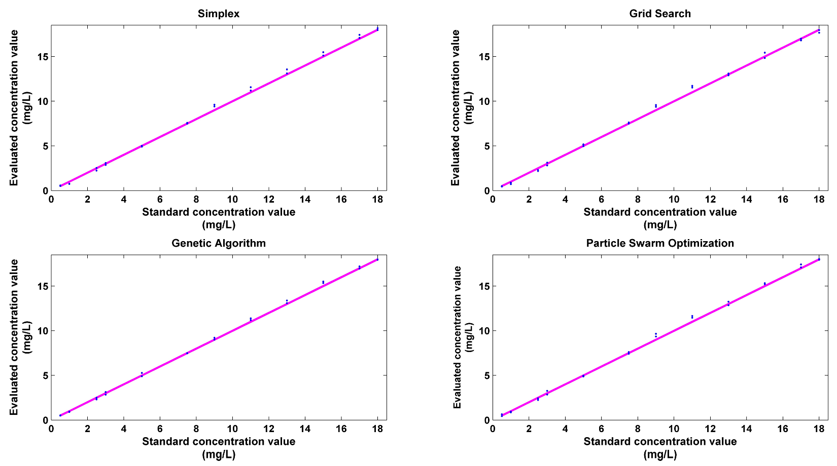
Figure 6 shows an illustration of a visual comparison between the real value and prediction value by LS-SVM regression models with four parameter optimization algorithms. The values of the abscissa represent the labels of testing set, and the values of ordinate represent the concentrations values (both real concentration values and prediction values based on different parameter optimization algorithms) of contaminants.
The curve marked with plus signs is the real concentration value of potassium ferricyanide, while the curves marked with squares, crosses, and triangles are the prediction values by the simplex-LSSVM, GS-LSSVM, and PSO-LS-SVM models, respectively. The result predicted by the GA-LSSVM model is marked with circles.
Table 5 presents the prediction performance of the test dataset in
Table 4 for each LS-SVM model. The RMSEP and r
2 of the testing set were obtained (
Table 5) using Equations (3) and (4).
In the table, RMSEP and r2 of the regression result for the testing dataset are acceptable when parameter optimization methods were used to obtain the best parameters for the LS-SVM training, whereas the model obtained by GA-LSSVM has the best generalization ability because of the high parallelism degree and strong adaptability of the genetic algorithm.
To test the performance of the described approach, two other models, LSSVM and multiple linear regression models, are also developed for comparison purposes. The LS-SVM model obtained by using the parameter optimization method performed better in terms of accuracy and generalization ability. In detail, the LS-SVM model produces a RMSEP of 1.3158 and an r2 of 0.9712, while the multiple linear regression models generate a RMSEP of 2.5327 and an r2 of 0.8531. As the RMSE indicator illustrates, compared with that of LS-SVM with default model parameters, the predictive error of PSO-LSSVM and GA-LSSVM decreases by 82.4% and 85.9%, respectively, proving that the proposed method provides good concentration prediction accuracy for quantitative evaluation of a known contaminant.
The aforementioned regression models were built with a five-dimension vector input. During the experiment, NH
3-N had minimal response to the contaminant solution, of which the concentration was 1 mg/L, 0.5 mg/L, or even less. The relative response value recorded in
Table 4 was 0.9365 mg/L when the concentration of potassium ferricyanide was 0.5 mg/L, which was possibly an illusion caused by noise fluctuation of water quality after response time. These potential errors were not eliminated because noise may arise anytime in a real-time sense, and the model obtained by the proposed method should have the robustness to handle small errors in one dimension of a five-dimension input model.
4.4. Analysis of Noise Source and Detection Limit
A common question for the regression modeling problem is how to discriminate the influence of environmental noise included in characteristics and how to determine model input dimensions.
Figure 7 shows the response curve for potassium ferricyanide with concentrations of 0.5 and 1.0 mg L
−1. Introduced by equipment noises mainly, lots of peaks and troughs exist in the graphs of turbidity, conductivity, and DO. These noises are independent and not related to contamination injections. This result is verified by the weak Pearson correlation coefficients for turbidity, conductivity, and DO (
Table 3), and also indicates that turbidity, conductivity, and DO does not respond to the presence of potassium ferricyanide.
As the input of the LS-SVM regression model, the relative response value is also a characteristic value extracted from the experimental data. The extraction refers to two parameters: baseline value and maximum response value, both of which may be responsible for deviation of results. For example, as shown in
Figure 7 some peaks and troughs during response time (e.g., marked in the graph of COD, TOC, and NO
3-N) shifted significantly from the previous reading because of equipment noise. This type of shift is difficult to predict, and a significant deviation between response value and baseline value occurs for real-time quantitative analysis. The baseline value relates to the window size and right boundary of the moving average model. Quantitative evaluation of water quality detection occurs immediately after the qualitative analysis, which includes contamination detection and contamination identification. When the detection decision is made, the right boundary of the moving average model is determined.
In the present study, we focus on the quantitative evaluation of contaminant concentrations but not contamination event detection; thus, the injection time of contaminations is chosen as the right boundary. Meanwhile, window size denotes the number of data involved in the calculation of the baseline value. Given the relative stability of the baseline, the window size need not be extremely large. With the autoregressive moving average method reported by Hou [
43] for comparison, a greater demand for historical data is observed because the input data of the autoregressive moving model should be thousands of orders of magnitude.
As mentioned in the last section, NH3-N had a minimal response to the contaminant solution when the concentration was 1 mg/L, 0.5 mg/L, or even less. As predicted for the two concentrations in the test set, only four of the five dimension inputs were useful, while NH3-N may change to an abnormal input, which caused prediction errors. Meanwhile, 0.5 mg/L and 1 mg/L were out of the range of the training set, which was from 2 mg/L to 18 mg/L, leading to several regression errors. Because of the adaptive and autocorrelation analysis of GA, GA-LSSVM has better generalization ability. However, regardless of what optimization method is used, a lower detection limit is defined, which is 0.5 mg/L in our study. Improving the generalization ability to improve the prediction accuracy around the detection limit by sacrificing the accuracy of the model is unnecessary.


