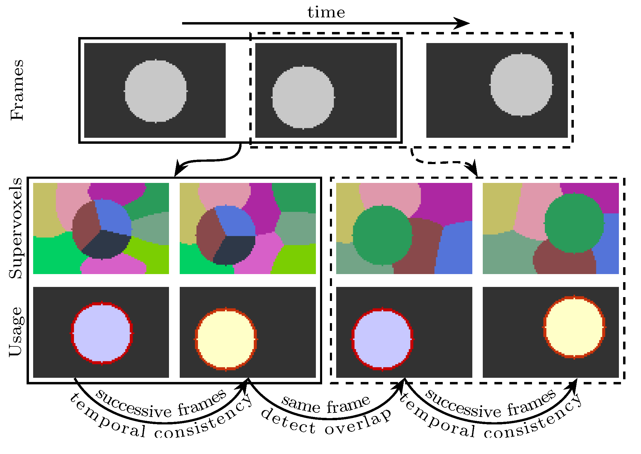
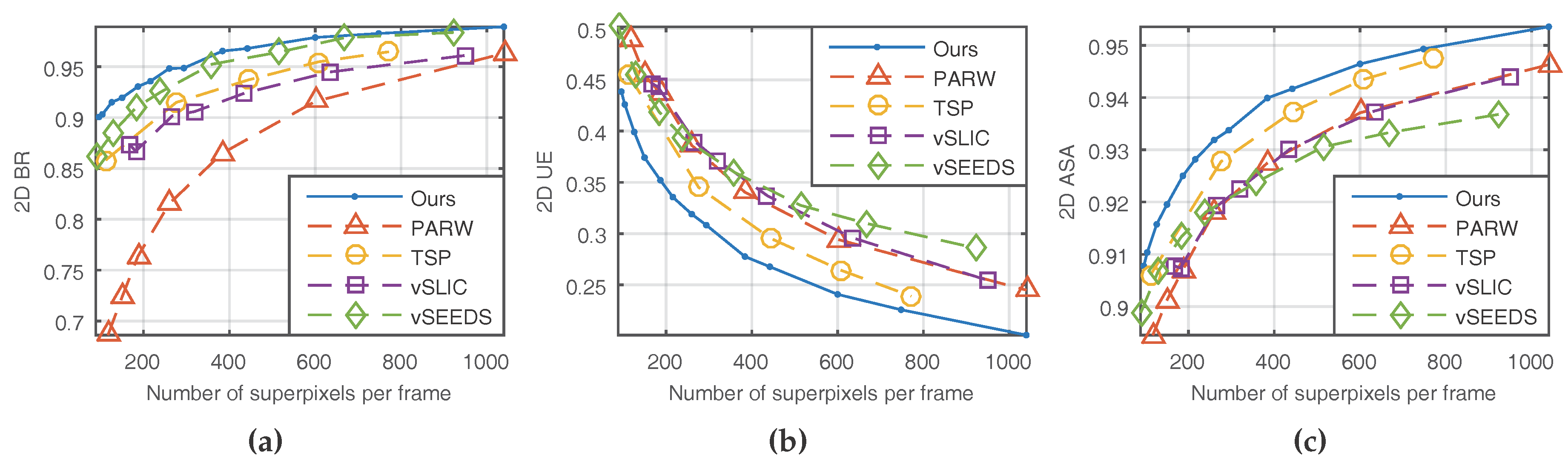
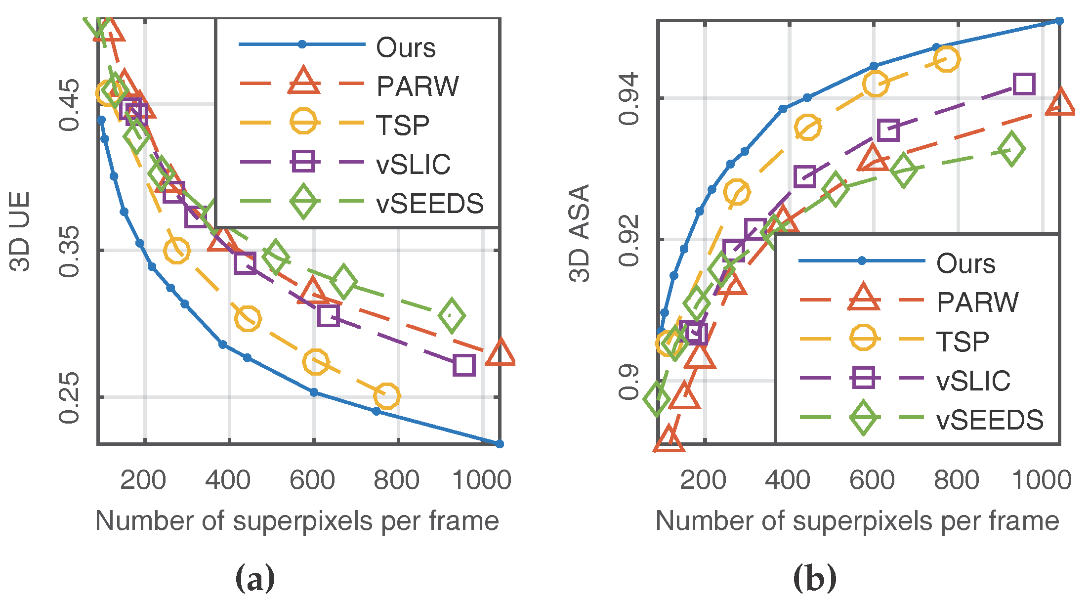
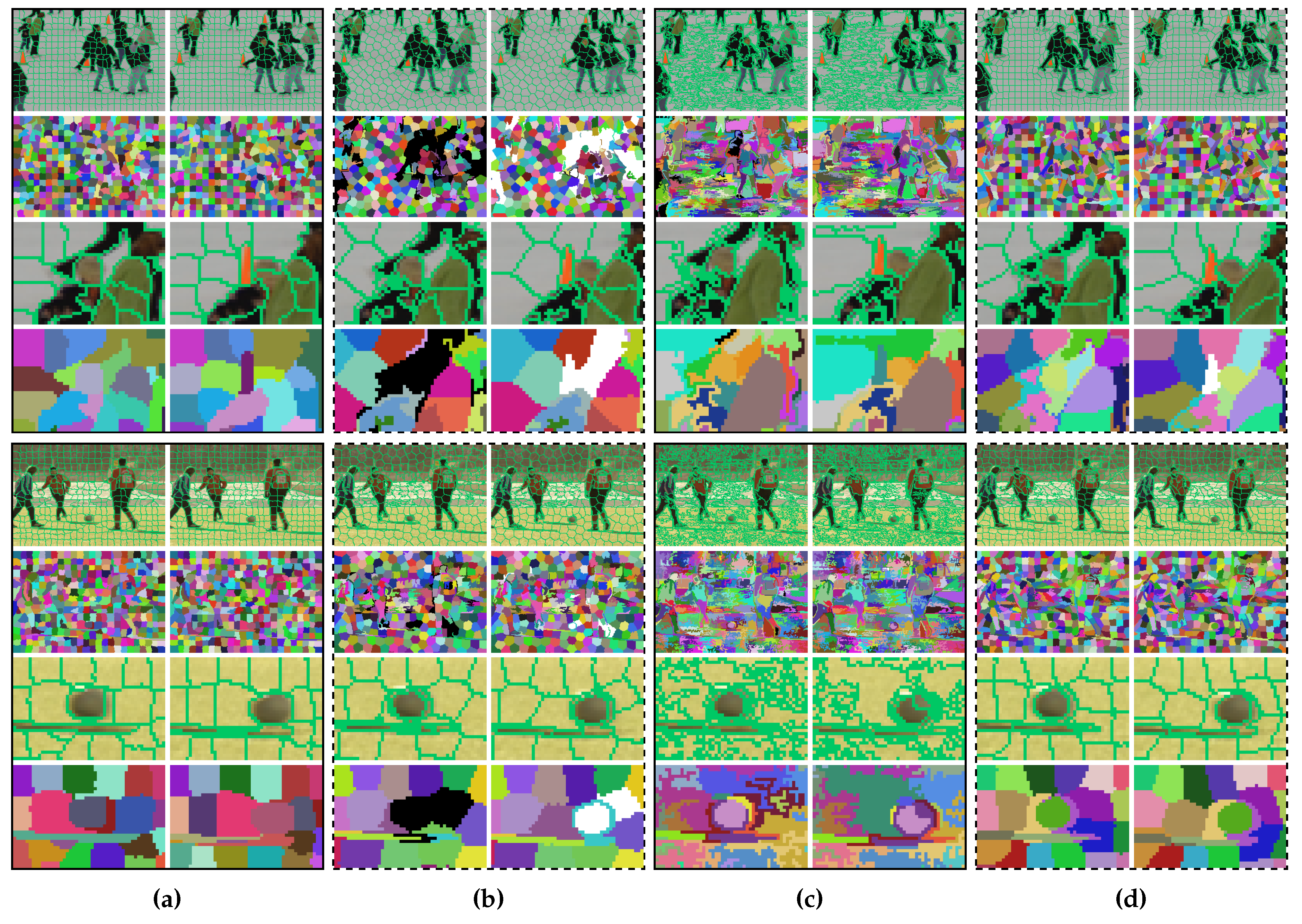
In the proposed method, the supervoxel problem is simplified as supervoxel segmentation on two adjacent frames (see
Figure 2 for an illustration). Each voxel is represented by a five-dimensional vector, in which the time property is not involved. Inspired by Ref. [
13], the time property of each voxel is modeled in an implicit fashion such that data points are organized in subspaces: one color subspace and two spatial subspaces (each frame has one spatial subspace). Each supervoxel is composed of two superpixels, each of which is associated to a Gaussian distribution with unknown parameters. To estimate the parameters, voxels are assumed to be observed from a mixture of Gaussian distributions. Based on maximum likelihood estimation, the unknown parameters are estimated using the expectation–maximization (EM) method. Once the values of the parameters are obtained, each voxel’s supervoxel label is determined to be the one that has the maximum posterior probability.
3.1. Problem Formulation
For a given sequence of frames, we use to denote pixel i in frame t, with and , where is the pixel index set and T is the frame set. The symbol denotes the number of elements in a given set; e.g., is the number of pixels in each frame, and is the number of frames. The width and height of the frames are denoted by W and H, respectively. Hence, we have .
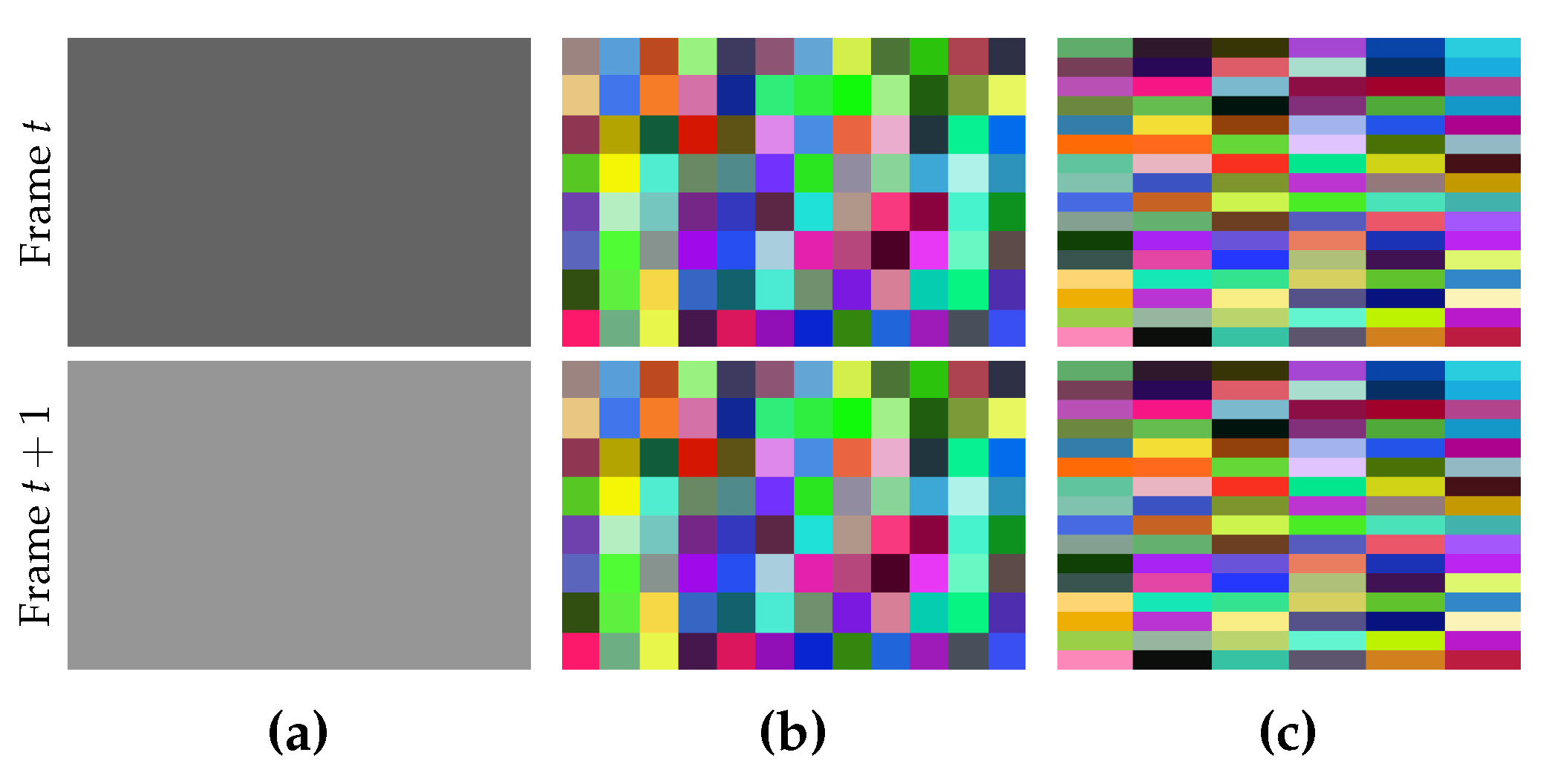
The desired size of each superpixel in a given frame is specified by
, where
and
are the number of pixels along width and height, respectively. Usually, the values of
and
are given by users. If we use values with a large difference, the shape of the generated superpixels in each frame will tend to be a narrow rectangle (see
Figure 3). Although people can assign different values to them, it is encouraged to assign the same value, or at least two different values with a very small difference, unless the narrow shape is useful for a special purpose.
Supervoxel segmentation is to assign each voxel a unique label. Voxels with the same label form a supervoxel. All the possible supervoxel labels form a supervoxel set
, where
is the number of supervoxels, which is computed in Equation (
1):
where
and
are the desired numbers of superpixels along width and height for a single frame. For simplicity, we assume
and
.
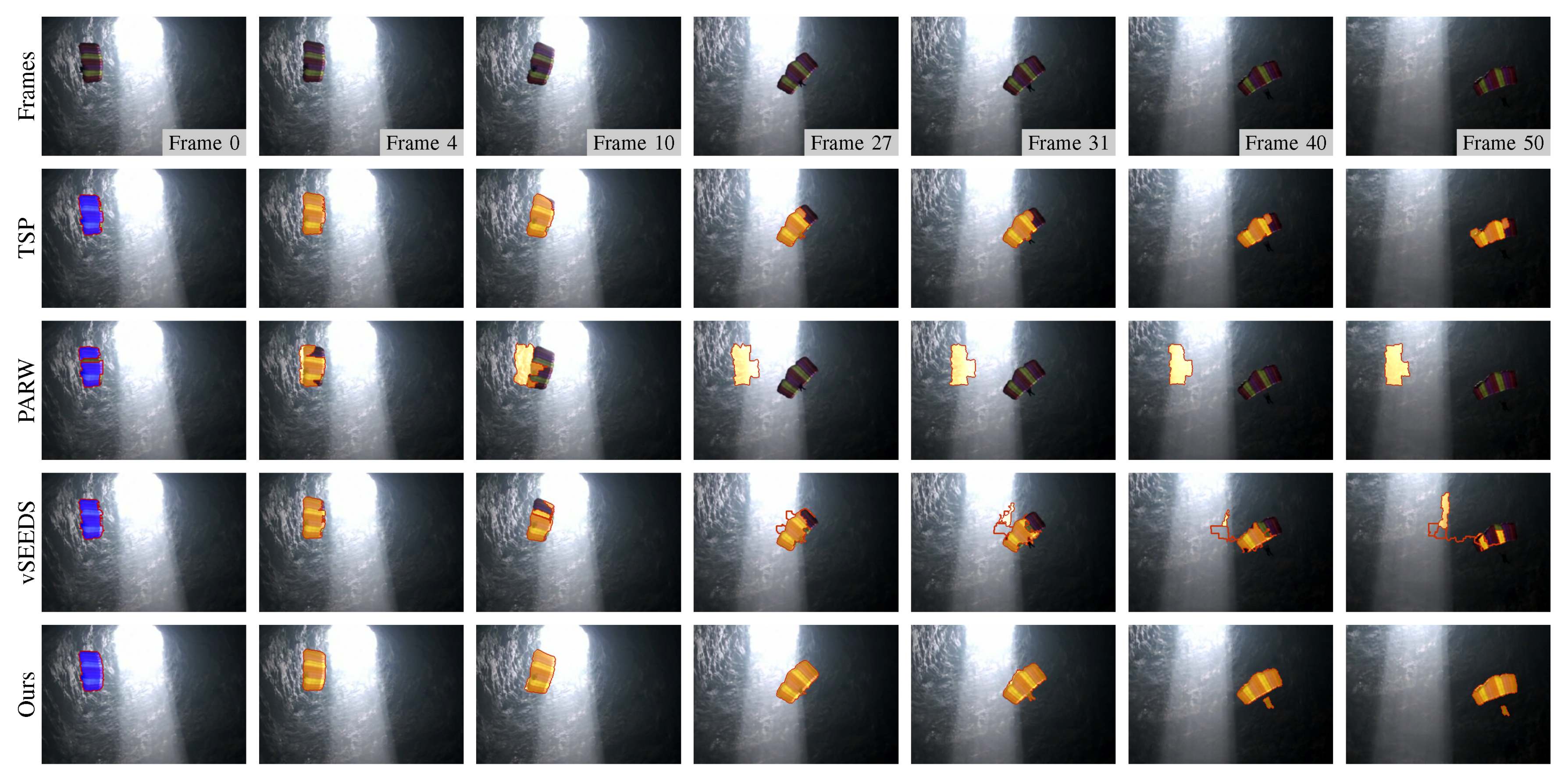
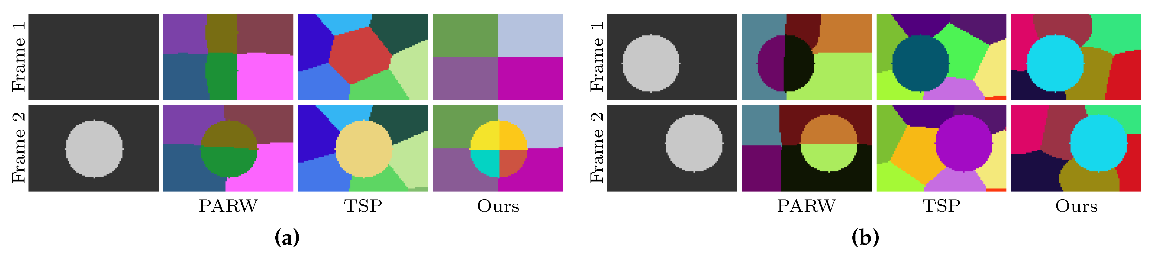
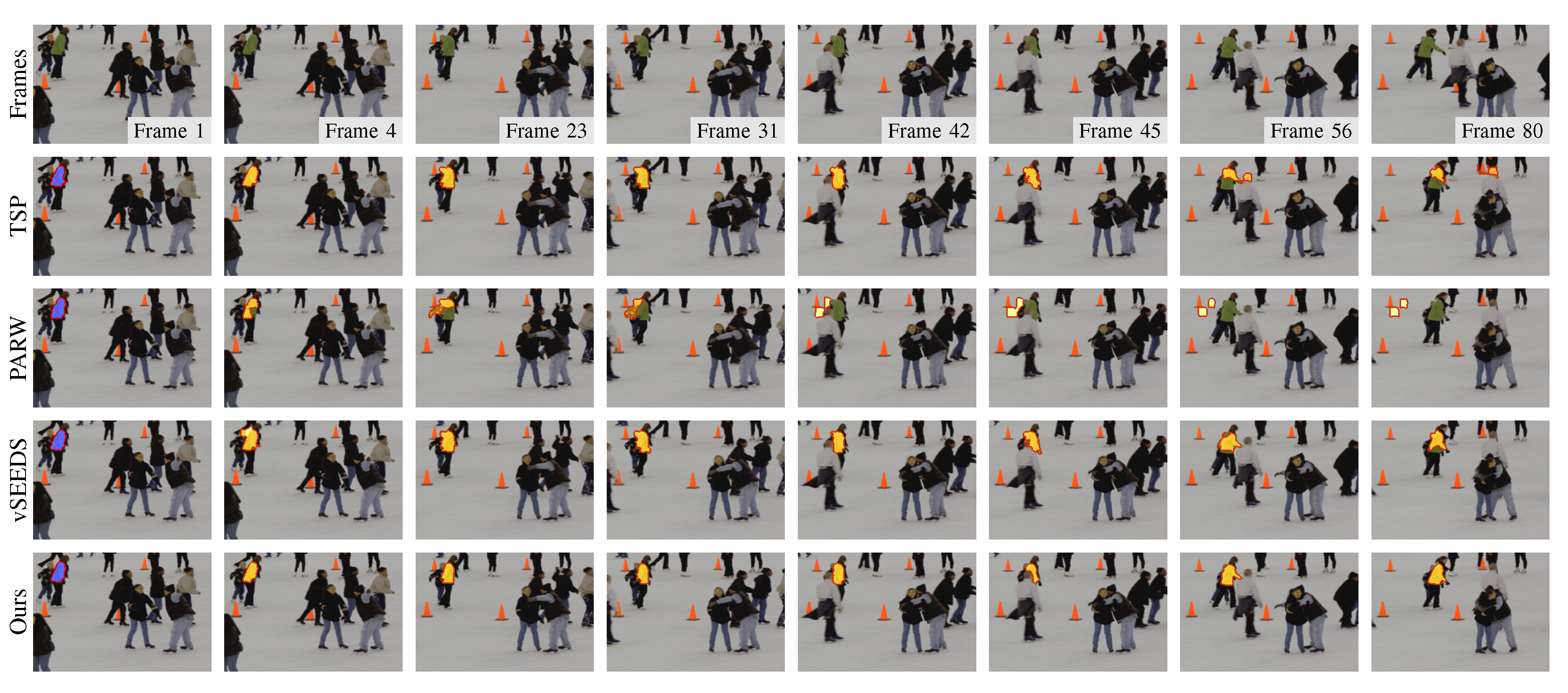
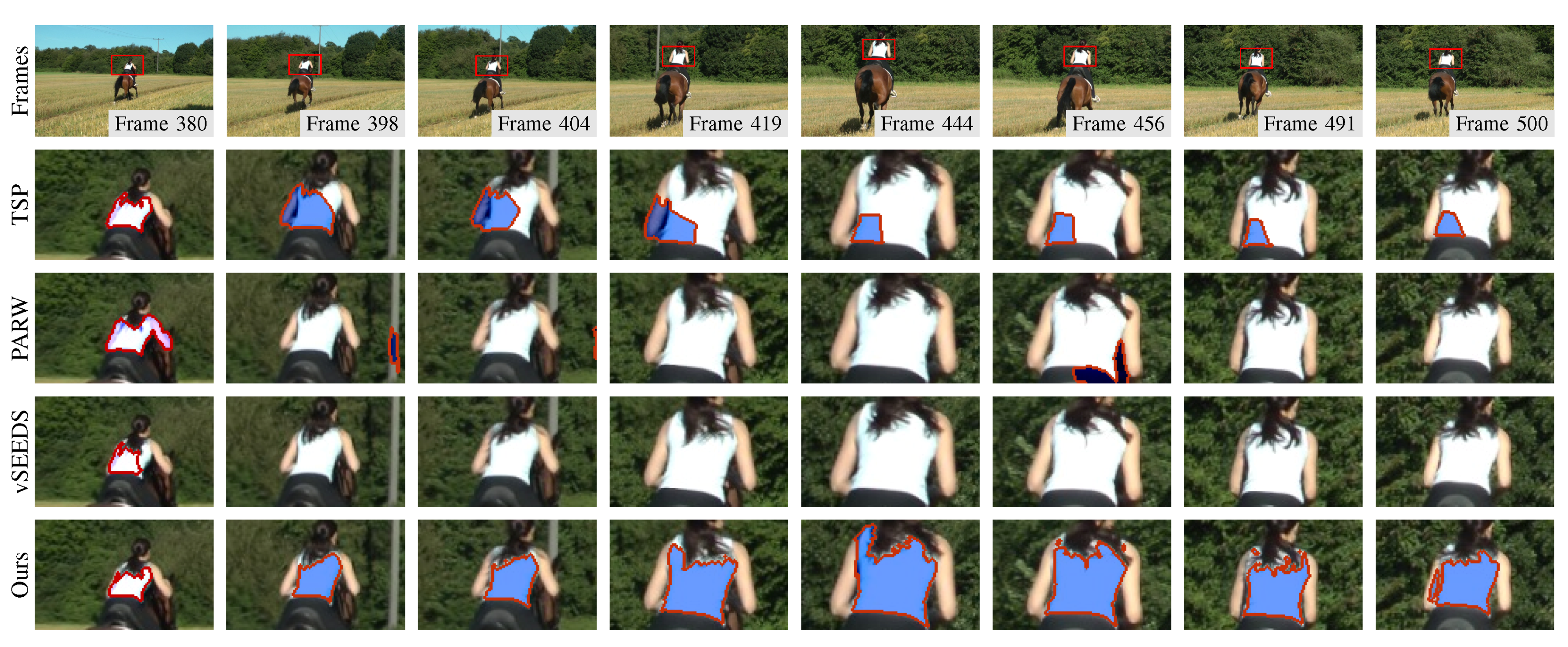
In this work, the supervoxel segmentation procedure is performed on every two frames. Therefore, a supervoxel is only valid on two successive frames. For instance, if some voxels in frame
t and frame
share the same supervoxel label, they are a subset of the same supervoxel. However, if the voxels are in frame
t and frame
, they are not in the same supervoxel. In order to provide cues for some subsequent applications (e.g., object tracking), frame
t—where
and
—will be used two times. In the first time, the segmentation is performed on frame
and frame
t. In the second time, the same procedure of segmentation is performed on frames
t and
. By doing this, frame
t will have two valid superpixel segmentations. The detected regions in frame
t can be propagated by finding the overlapping superpixels in the second segmentation (see
Figure 2 for an illustration). Because the same methods are used to segment any two frames, the supervoxel problem becomes finding
K supervoxels for frame
t and
such that the generated supervoxels are similar in size, adhere to object boundaries well, and are temporally consistent. Therefore, only frame
t and frame
will be considered in
Section 3.2.
3.2. The Model
To distinguish variables between two frames, a symbol with a hat at its top indicates that the symbol is related to frame
. Each voxel in frame
t is represented by a five-dimensional vector including spatial location
and three CIELAB color components—lightness
and two color components
and
. This can be expressed by
in which the superscript
T indicates vector transpose. Similarly, voxel
i in frame
is represented using
For two given frames
t and
, voxels are assumed to be distributed according to mixtures of Gaussian distributions in which each Gaussian distribution corresponds to a superpixel. Gaussian function
is defined in Equation (
4), where the semicolon is used to separate variables and parameters:
in which
z is a
D-dimensional column vector,
and
are mean vector and covariance matrix, respectively.
Generally, if voxels in different frames have similar colors and have small spatial distances, they generally belong to the same object. This is particularly true in the videos with moving objects. To incorporate this notion into our model, we use different parameters for spatial information but the same parameters for color information for the same supervoxel in the definition of voxel density functions
and
, as shown in Equation (
5). This is the key point to ensure temporal consistency:
in which
where
and
are spatial mean vectors and spatial covariance matrices for frame
t with
. Their parallel notations
and
are for frame
. The color mean vectors
and color covariance matrices
are for both frame
t and frame
. Supervoxel
k can be characterized by the parameters
,
,
,
,
, and
, and thus each supervoxel corresponds to two Gaussian distributions. Accounting for the locality of supervoxels,
in Equation (
5) is a subset of
, and its elements are related to the spatial location of voxel
i. The definition of
will be discussed later. Instead of defining
as a variable just like existing Gaussian mixture models,
is defined as a constant
here to make the generated supervoxels similar in size.
Once two successive frames
t and
are given, parameters in the Gaussian densities can be inferred and the label of each voxel,
for frame
t and
for frame
, will be determined by the following equations:
in which
is the probability of assigning voxel
i in frame
t to supervoxel
k given the observation
.
has a similar meaning. By applying Bayes rule, the posterior probabilities in Equation (
7) can be expressed by
Based on Equations (
7) and (
8),
and
can be computed by the equivalent equations, as shown below:
3.3. Estimating Parameters of Gaussian Distributions
Given two frames
t and
, we use the method of maximum likelihood to estimate the unknown parameters in the Gaussian distributions. Since the proposed density functions for voxels may be not identical because the elements in
may be different for different
(see
Section 3.4 for details), updating formulas for traditional GMM cannot be simply copied to our new model. Therefore, we will derive the updating formulas for the proposed model in this section by applying the classical expectation–maximization (EM) method to iteratively improve the log-likelihood.
As the voxels in frames
t and
are assumed to be distributed independently, the log-likelihood
for the two frames can be written out as follows:
where
is a vector of all the unknown parameters composed of
,
,
,
,
, and
with
. For each supervoxel
k,
and
. Because the number of elements in supervoxel set
is constant (see
Section 3.4), the value of the parameter
that maximizes
is equal to the value that maximizes the following function
:
It is difficult to find the optimal value for by maximizing directly. We insert new variables and into Equation (12) such that
Then, Equation (12) will become Equation (14). By applying Jensen’s inequality, the EM method is to alternatively find
satisfying the equality of the inequality in Equation (15) with parameters in
being known (expectation step or E-step), and find parameters in
that maximize
which is defined in Equation (15) using the obtained
R (maximization step or M-step):
E-step: According to the theory of Jensen’s inequality, equality holds if and only if
are constant. With the constraints in Equation (13), formulas to update
R can be derived by eliminating the temporal variables
and
in Equation (16), as shown below:
where
is defined in
Section 3.4.
M-step: To find the parameters
that maximize
, we first get the partial derivatives of
with respect to different components of
, as shown in Equations (18)–(22), and then set them to zero to get the optimal
, which is shown in Equations (24)–(27):
where
and
are spatial vectors of voxel
i in frame
t and
, respectively. Similarly,
and
are color vectors. For each supervoxel
k,
is a voxel set that supervoxel
k may cover, and is deduced from
as shown in Equation (23):
Usually, the EM method starts by feeding it with a guess of the parameters in . Then, R and will be alternatively updated using the formulas mentioned in E-step and M-step. However, there is a risk that the covariance matrices may become singular and we may fail to obtain their inverse matrices. For example, when the voxels in have the same constant color, during the iteration of EM will become zero matrix, which is obviously singular. To avoid this trouble, one can perturb each and each with a small random vector before the EM iterations. This trick may succeed in most cases, but it may fail when an object in a frame is very narrow (e.g., a straight line), in which case certain covariance matrices or may become singular. In order to prevent the covariance matrices from being singular, we first obtain their eigenvalues and impose a lower bound to the eigenvalues to reproduce the covariance matrices. When an eigenvalue is less than the specified lower bound, we assign the eigenvalue to that lower bound. We use and to denote the lower bound of spatial eigenvalues and color eigenvalues, respectively. Experimentally, we have found that and is appropriate to outperform the state-of-the-art algorithms. We will use this setting for the remaining text.
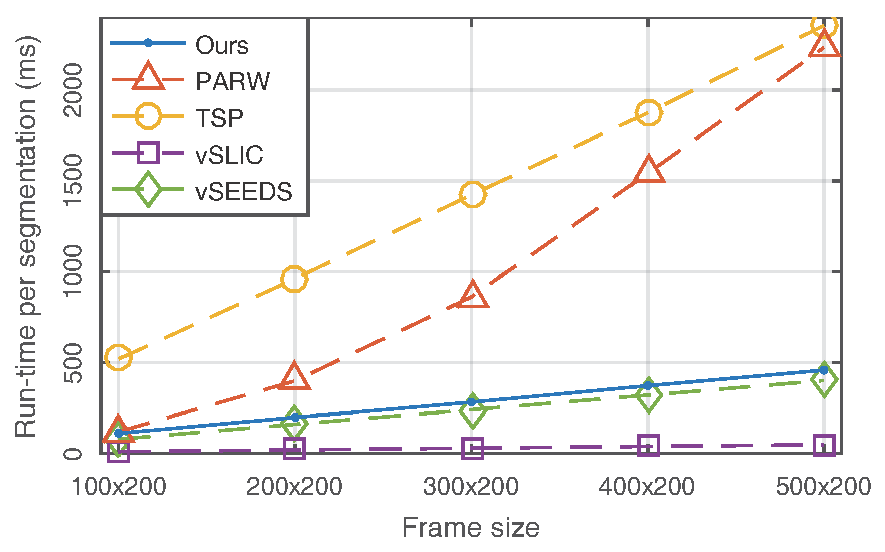
In theory, the iteration of the EM method will not stop until the parameters in converge. However, EM needs hundreds of iterations to reach the condition of convergence, resulting in a low computational efficiency. In practice, aiming to reduce run-time, we use a fixed number of iterations , which is sufficient in practice for generating supervoxels with state-of-the-art accuracy.
3.4. Defining and Initializing
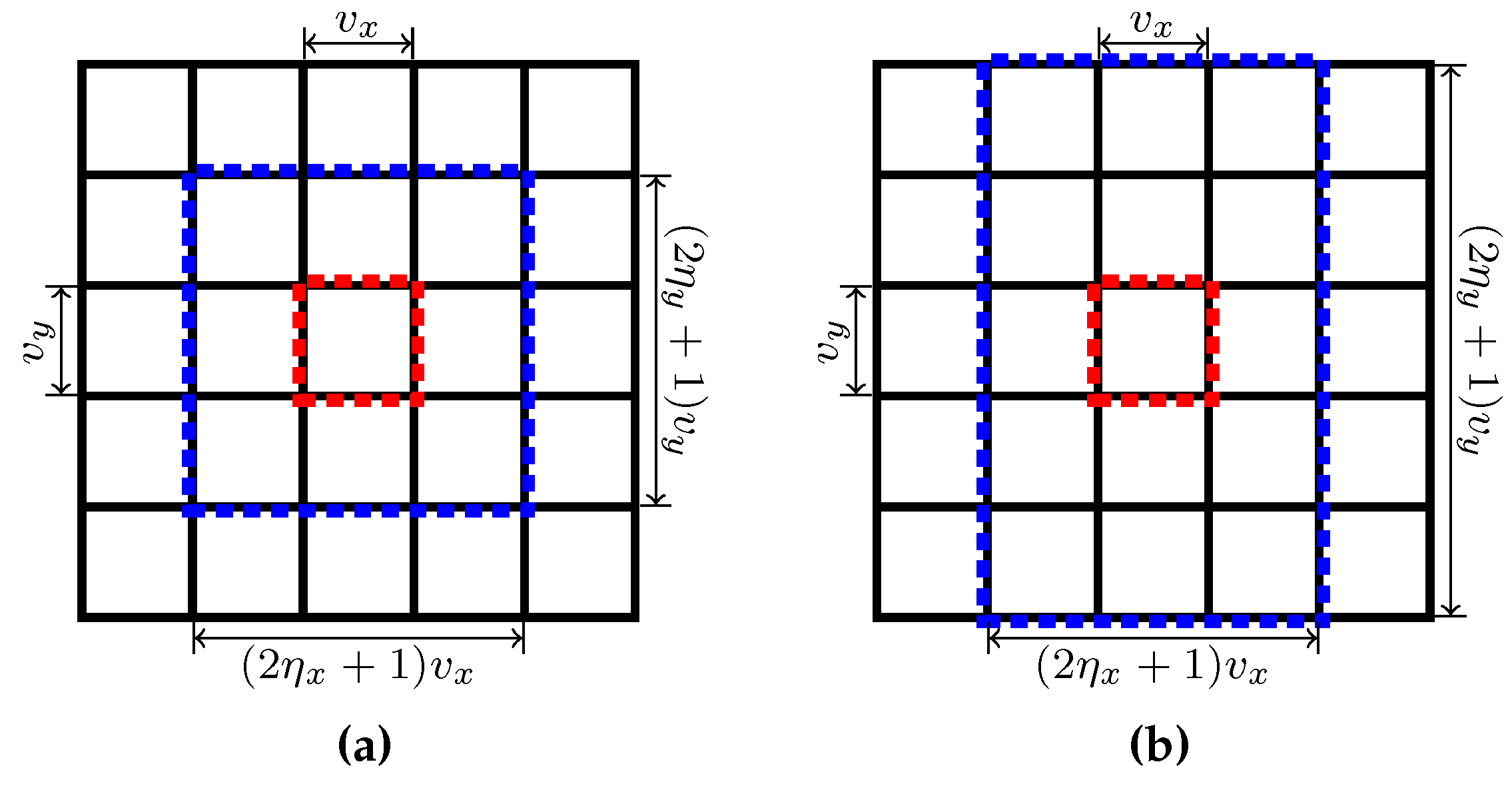
The definition of supervoxel subsets
of
will be discussed in this section using mainly the notations mentioned in
Section 3.1. After the value of
and
are assigned, we define
rectangle regions called
anchor regions, with each anchor region corresponding to a supervoxel. As illustrated in
Figure 4, for each frame, an anchor region contains
voxels and all the anchor regions are regularly placed on every frame. For a given supervoxel
k, all voxels in its anchor region are assigned an
anchor label . Then,
is defined using the anchor label of voxel
i using the following equations:
where
and
are parameters used to control the number of supervoxels from which each voxel
i may be generated. Clearly, at least one of the two parameters must be greater than or equal to 1.
Recall the definition of
in Equation (23) of
Section 3.3. Elements of
are in turn determined by
. The voxel set
is called the
k-th supervoxel’s
overlap region, into which voxels in supervoxel
k may spread. With the help of
Figure 4, it is easy to conclude that an overlap region
of a supervoxel
k is the region whose center is the anchor region of the supervoxel
k and whose width and height can be divided evenly by
and
respectively, and can be expressed by
and
using
and
. There are some exceptions, however. When an anchor region
k is at the boundary of a frame, the size of
may be less than
, but is at least
, which is the case in which the anchor region is at one of the four corners of the frame. This conclusion can be used to deduce the computational complexity of our algorithm. As discussed in
Section 3.5, the computational complexity can be affected by
and
. A large value for
will increase the run-time of the algorithm. Meanwhile, a large value for
indicates that a supervoxel has a large overlap region, which may result in a better performance in temporal consistency. By default, we use
for our experiments.
In our model, a Gaussian distribution represents a superpixel in a single frame, and two Gaussian distributions with the same color parameters (color mean vector and color covariance matrix) but with different spatial parameters represent a single supervoxel. As we expect that the generated superpixels are regularly distributed on each frame, it is straightforward to initialize and using the center of the k-th anchor region. Since a color mean vector varies according to the color information of two frames (see Equation (26)) during the EM iterations, the is initialized by the mean color of the two voxels at the center of the k-th anchor region of each frame.
For each supervoxel
k, the corresponding covariance matrices serve as normalizers for the squares of the Euclidean distances (refer to Equations (
4) and (
9)). To initialize each of the covariance matrices, the idea is to assign their diagonals with the same value, which can be interpreted as a distance within which two voxels tend to be in the same supervoxel. We have found that it is sufficient to initialize color covariance matrices with a color distance
(see Equation (30)) and a small perturbation for
affects the result less. As we hope each superpixel for a single frame will have the same size
, the spatial covariance matrices can be initialized using Equation (30):
3.5. Computational Complexity
With the discussion above, for any two successive frames, the proposed algorithm can be summarized in Algorithm 1. The proposed algorithm is composed of three major procedures, initializing
(line 1 to line 3), updating
R (line 5 to line 9), and updating
(line 10 to line 13). It is obvious that the initialization of
needs a computational cost of
, where
K is the number of desired supervoxels in two frames and is originally defined in Equation (
1).
| Algorithm 1 The proposed supervoxel algorithm. |
Input: and , two successive frames.
Output: and , .
1: for all do
2: Initialize , , , , , (refer to Section 3.4).
3: end for
4: for to M do {refer to Section 3.3 for the value of M}
5: for all do
6: for all do {refer to Section 3.4 for }
7: Update and using Equation (17).
8: end for
9: end for
10: for all do
11: Update , , and using Equations (24)–(26).
12: Update , and using Equations (24)–(27).
13: end for
14: end for
15: for all do
16: and are determined by Equation (9).
17: end for |
According to Equations (28) and (29), the number of elements in
satisfies the following inequality:
For each voxel
i, updating
or
,
needs time
. For all the elements in
R, we therefore have a computational complexity
. Based on Equations (24)–(27), for a given supervoxel
k, updating the parameters in
or
needs a time of
. By the conclusions about the size of
in
Section 3.4, we know that
Therefore, the computational complexity for updating
is
Because
and we use constant values for
and
, the computational complexity of our algorithm is
.
When the input video has more than two frames, every internal frame will have two segmentation results: one generated with its previous frame and another generated with its next frame (refer to
Figure 2 for a visual illustration). For the entire video sequence, the complexity is
, where
is the number of frames in the input video and has been mentioned in
Section 3.1.


