
A High Spatial Resolution Depth Sensing Method Based on Binocular Structured Light

1
The Institute of Artificial Intelligence and Robotics, Xi’an Jiaotong University, Xi’an 710049, China
2
The National Engineering Laboratory for Visual Information Processing and Applications, Xi’an Jiaotong University, Xi’an 710049, China
3
Shaanxi Provincial Key Laboratory of Digital Technology and Intelligent Systems, Xi’an 710049, China
*
Author to whom correspondence should be addressed.
Sensors 2017, 17(4), 805; https://doi.org/10.3390/s17040805
Submission received: 17 January 2017
/
Revised: 30 March 2017
/
Accepted: 5 April 2017
/
Published: 8 April 2017
(This article belongs to the Section Physical Sensors)
Abstract
:Depth information has been used in many fields because of its low cost and easy availability, since the Microsoft Kinect was released. However, the Kinect and Kinect-like RGB-D sensors show limited performance in certain applications and place high demands on accuracy and robustness of depth information. In this paper, we propose a depth sensing system that contains a laser projector similar to that used in the Kinect, and two infrared cameras located on both sides of the laser projector, to obtain higher spatial resolution depth information. We apply the block-matching algorithm to estimate the disparity. To improve the spatial resolution, we reduce the size of matching blocks, but smaller matching blocks generate lower matching precision. To address this problem, we combine two matching modes (binocular mode and monocular mode) in the disparity estimation process. Experimental results show that our method can obtain higher spatial resolution depth without loss of the quality of the range image, compared with the Kinect. Furthermore, our algorithm is implemented on a low-cost hardware platform, and the system can support the resolution of 1280 × 960, and up to a speed of 60 frames per second, for depth image sequences.
1. Introduction
At present, human computer interaction based on three-dimensional (3D) depth information has become highly attractive in the areas of image processing and computer vision, which further promotes the development of 3D depth acquisition technology. In addition, the recently developed 3D depth sensors, such as the Microsoft Kinect (Microsoft Corporation, Redmond, Washington, DC, USA) [1], have been applied in more fields, such as gesture recognition [2,3,4,5], intelligent driving [6,7], surveillance [8], 3D reconstruction [9,10], and so on. 3D depth acquisition technology measures the distance information between objects and a depth sensor. It represents a non-contact, non-destructive measurement technology.
The fully studied methods for acquiring depth information can be classified into two categories: passive methods and active methods.
Binocular stereo vision is an active research topic in passive methods. Some authors [11,12] have implemented an entire stereo vision process on a hardware platform accompanied by progress of the algorithms and field programmable gate array (FPGA) technology. However, the considerable computational expense still limits its industrialization, as some algorithms have to be realized on a custom-build FPGA. One the other hand, stereo vision still does not have a good method to acquire the dense disparity map for a large textureless area, such as a white wall. Therefore, no related electronic products have yet been released.
Time-of-Flight (ToF) and structured light [13,14] is mainly used in the active depth sensing method. The ToF technology acquires the distance information based on measuring the flight time along the light path. Samsung released the first complementary metal oxide semiconductor (CMOS)-based ToF sensor in 2012, where synchronized depth (480 × 360) and RGB images (1920 × 720) can be obtained by a single image sensor [15]. The Kinect 2 (Kinect for XBox One) issued in 2013 by Microsoft is also based on the ToF principle [16]. However, in terms of miniaturization and integration, the advantages of technology based on structured light are not ignored. In addition to the Microsoft Kinect, other companies have also researched and released their own depth-sensing cameras, or intend to integrate them into their electronic products. For example, in 2013 Apple purchased Primesense and claim an important invention patent: “Depth Perception Device and System” [17], and intends to employ it as an input device for human–machine interfaces for their product. In early 2014, Intel announced a three-dimensional depth imaging device, the “RealSense 3D Camera,” and the products RealSense R200 and SR300 have been on the market since 2016. In February 2014, Google announced a new project “Tango,” which intends to make a smartphone with 3D visual recognition capabilities. In 2015, the Microsoft holographic visor “Hololens” appeared on the market.
However, the depth-sensing systems based on structured light are not mature when compared to two-dimensional (2D) imaging systems. The resolution and accuracy of the depth image are lower, and the performance is not very reliable in the use of moving objects or dynamic scenes. In [18,19], the authors combine color images to restore the corresponding depth image. The methods can improve the image quality and reduce the noise of the acquired depth map, but the improvement of the measurement precision is limited.
Moreover, the hardware implementation of depth sensors based on structured light remains a black box, to a large extent, in the literature. In [20], we have proposed a full very large scale integration (VLSI) implementation method to obtain a high-resolution and high-accuracy depth map based on randomized speckle patterns. Then it was found that the spatial resolution of the depth map has the potential to be further improved. Thus, in this paper, we add an infrared camera at the right of the laser projector and employ the local binocular stereo matching algorithm to improve the performance of the depth map.
Several binocular structured light approaches have been proposed for acquiring a disparity map. Different projected patterns and disparity estimation methods are employed. Ma et al. combined a color-coded pattern based on vertical stripes and the semi-global stereo matching (SGM) algorithm to obtain a dense facial disparity map [21]. An et al. provided the comparative analysis of various structured lighting techniques with a view for facial reconstruction [22]. Nguyen et al. employed the dot-coded pattern to enhance textures on plants, and five pairs of RGB cameras to reconstruct the whole plants [23]. In this system, stereo block matching is applied to calculate the matching results. The gray or color-coded patterns mentioned above are sensible to ambient light and the surface color of objects. Yang et al. used the light stripes and corresponding decoding method to measure the 3D surfaces [24]. However, this method is not suitable for moving objects. The experimental setup proposed by Dekiff et al. also used the speckle pattern and digital image correlation [25]. There is a triangulation angle of about 30° between the two cameras. It is a short-range measurement system. The measuring distance is under 1 m and the size of the measuring field is approximately 24 cm × 18 cm. The Intel RealSense Camera SR300 includes two infrared cameras and has similar performance.
Our key contribution in this paper, beyond [20], is that an infrared camera is added at the right of the laser projector, then the binocular matching mode, performed between the captured left and right patterns, is employed to improve the spatial resolution in the X-Y direction. The mismatching and occlusion is unavoidable in the binocular matching process, so the monocular matching mode, performed between the left and the reference patterns, is also employed to revise the matching results. Finally, the complete system is implemented and verified on a low-cost hardware platform with a laser projector and two-camera setup.
The rest of this paper is organized as follows: In Section 2, the basic principles mentioned in our depth-sensing method are briefly introduced. The acquisition steps of the depth map from projected speckle patterns are described in Section 3. Section 4 gives the full-pipeline architecture of our proposed method. Section 5 discusses the utility of our method and presents some simulation results. The paper ends with some conclusions in Section 6.
2. Related Ranging Principles
In [20], a consistency enhancement algorithm is proposed to make the intensity of the pattern formed at different distances as consistent as possible so as to ensure the matching accuracy in the disparity estimation process. However, the surface material of the objects also affects the projected pattern, so we have to select a larger block, compared with the smallest size in theory, to perform the block-matching step. Therefore, we add an infrared camera at the right of the laser projector in order to capture a pattern that is nearly consistent with the captured left pattern. Then the smallest image block can be employed in the binocular matching mode performed between the captured left and right patterns so as to improve the spatial resolution of the depth map.
Figure 1 shows the position relationship between the projector and cameras. One camera is added to the right of the laser projector compared with traditional depth-sensing method. The experimental platform contains a projector which projects a speckle pattern similar to that used in the Kinect and two cameras with the same performance parameters. The projector is between the two cameras. The three units are located in the same straight line and the optical axes of each are parallel. In our depth-sensing method, the triangulation principle and digital image correlation (DIC) are related. The triangulation principle is to transform the disparity to distance information through the geometrical relationship. Generally, the digital image correlation (DIC) is performed to identify the corresponding points in the individual images.
2.1. Triangulation Principle
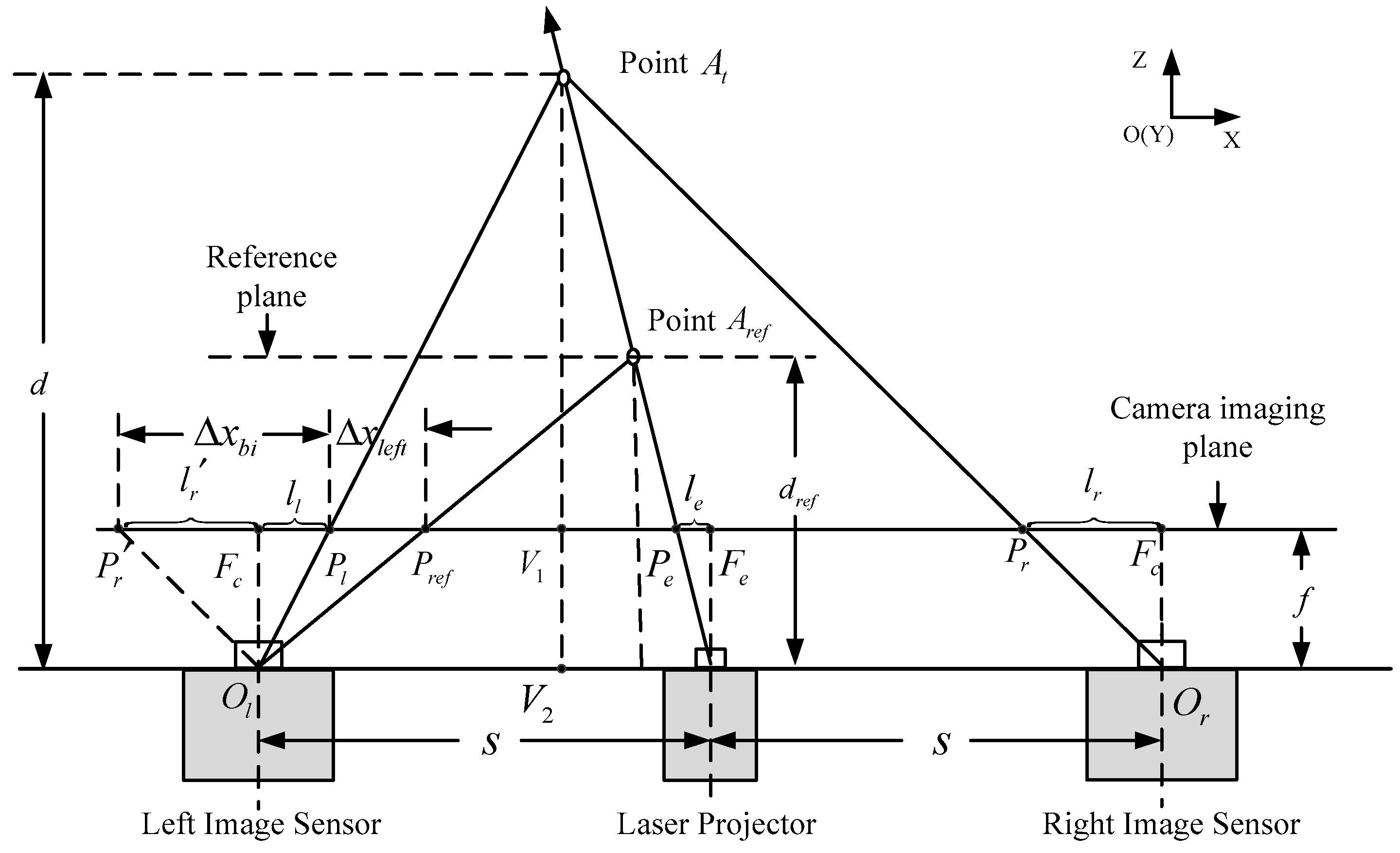
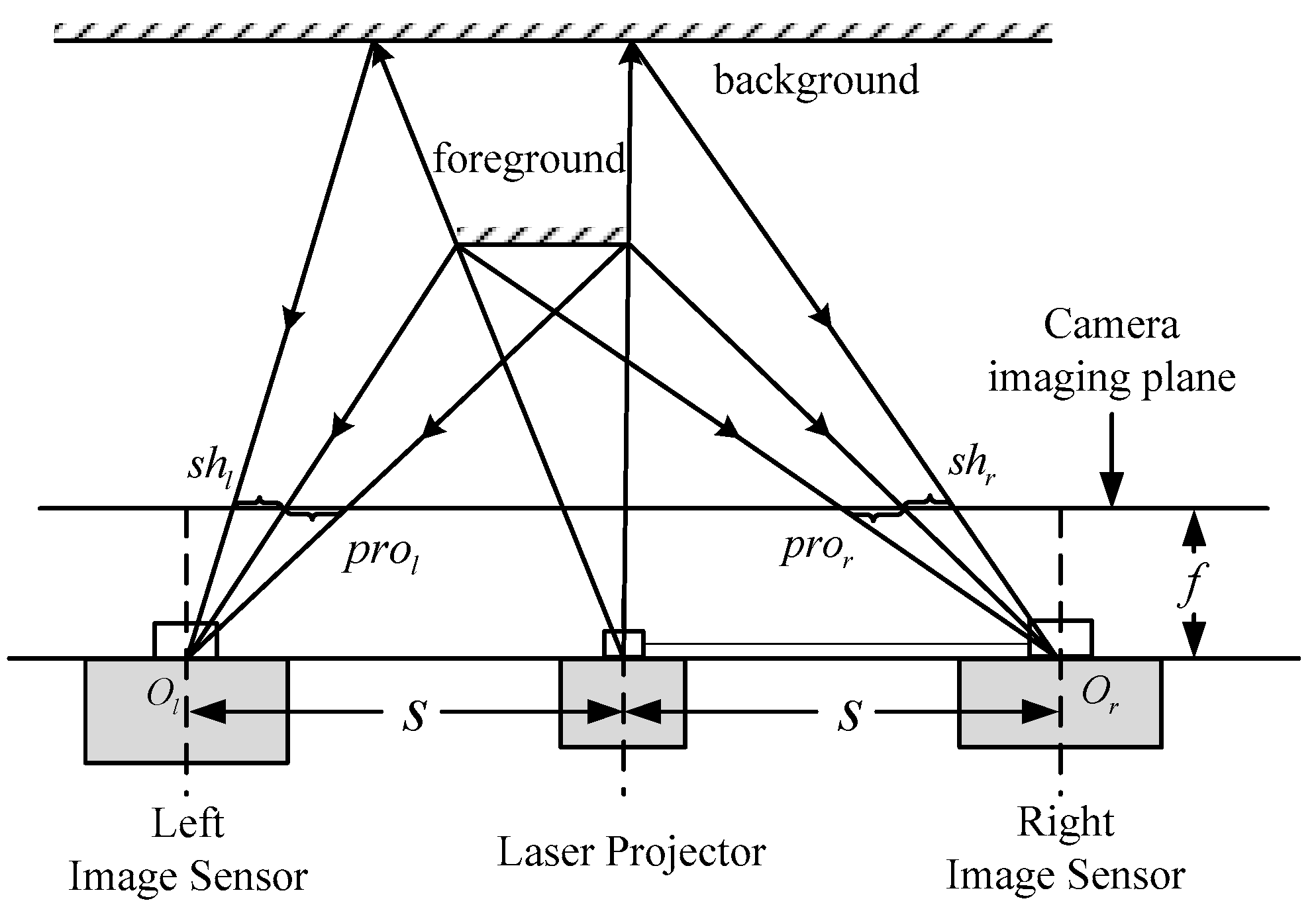
In the binocular stereo system, the problem of occlusion is unavoidable. Thus, we combine the monocular ranging method to compensate for the disparity of the occluded areas. In this section, the ranging principle and the transformation relationship of the two displacement vectors from two modes are introduced. The ranging method is based on the triangulation principle. As shown in Figure 2, point is an arbitrary point in the 3D space marked by the speckle pattern. The two points, and , respectively, are the projection of on the left and right camera imaging planes, so they are the corresponding image points of in the left and right two images. According to photogrammetry, if we obtain the displacement of the test point in two images, we can obtain the vertical distance from point to the ranging sensor. The two cameras are located as shown in Figure 1, and their coordinates only differ as per the translation distance in the X direction. Thus, the image planes of the two cameras are on the same plane, and the epipolar lines are aligned with the scanline of the image. Therefore, the displacement in the Y direction can be ignored, we only require an estimate of the displacement in the X direction between the projection point of on the left and right camera imaging planes. We assume that the optical focal length of the image sensor is , is the physical pixel-pitch, and is the baseline distance between the laser projector and image sensor. According to the relationship between similar triangles, we can obtain the proportional relationship , where the parameter is the distance between the sensor and the point . Then the depth value of point can be calculated as
where represents the displacement of the corresponding image points , , respectively, on the left and right images.
Next, the depth sensing technology with only the left-side camera is discussed. In the process, we need to acquire a reference image from the left camera at a known distance. As shown in Figure 2, the point is the position of point at the reference distance. According to the relationship between similar triangles, we can obtain the proportional relationship and . Then the depth value of point can be calculated as
where represents the displacement of the corresponding image points , , respectively, on the left and its reference images.
From Equations (1) and (2), we can observe that the inverse of distance follows a linear relationship with the displacement or ; thus, there is a simple linear relationship between the two disparities. The point can be located in front of, or behind, the reference point , so the value of displacement can be positive or negative. In this paper, we set a direction for the displacement. The projection point is assigned as the end point of the vector, and the projection point or as the start point of the vector. Then we can get and . Combining Equations (1) and (2), we can obtain the relationship of the two displacement as follows:
2.2. Digital Image Correlation
The digital image correlation (DIC) algorithm was developed at the end of last century and has been widely used to analyze deformation and identify the corresponding points between different images [25,26]. Its principle is to match subsets from different digital images by an appropriate similarity calculation method. The process is to ensure the parameters in the displacement shape function through a correlation function. The displacement mentioned in the Section 2.1 is contained in these parameters.
Assume that the coordinate of point in the first image (left speckle image) is . In order to determine the corresponding point in second image (right or reference speckle image), a square subset around the central point is extracted. Each point in the subset is represented by . If the represented subset’s surface is perpendicular to the optical axis, it only brings in rigid displacement; the mapping position in the second image of each point in this subset is calculated by:
where is the displacement of the subset center point in the X direction (the displacement in the Y direction can be ignored in our paper), while, in most situations, the speckle pattern projected on the tested object may be deformed. Thus we introduce the first-order displacement shape function to approximate the mapping position
where the parameters , are the components of the first-order displacement gradient. Lu and Cary [27] propose a DIC algorithm using a second-order displacement shape function for large deformations, but it has twelve parameters which increases the computational difficulty and complexity. Therefore, the displacement is estimated according to Equation (5). The block-matching algorithm is employed to estimate the displacement in Equations (4) and (5), which is also or in Section 2.1. In the implementation process, first we assign different initial values for parameters and , and then extract the different subsets with the size of from the second image. Finally, Equation (6) is employed as similarity criterion to find the optimal matching subsets:
where the , are, respectively, the discrete gray value of the first and second patterns.
The digital image correlation (DIC) algorithm is a local stereo matching algorithm. In addition to this algorithm, there are other stereo matching algorithms, such as semi-global block matching [28], belief propagation, graph cuts [29], and so on. However, these algorithms are not adaptable to our system. The reasons are as follows. Firstly, in the structured light ranging, the projected pattern is coded following a certain principle. The decoding method that is the ranging algorithm is designed according to the coding method. In this paper, the speckle pattern is binary, and composed of randomly distributed isolated speckles. Every image block extracted from the pattern is unique, so the block-matching algorithm is enough to decode the pattern. Secondly, other stereo matching algorithms are very complex and utilized to optimize the depth map, such as the problems of texturelessness and occlusion. In our paper, the infrared camera only can capture the projected image itself without additional information from the surrounding environment, such as the color or gray information. The edge information and other features of objects are very difficult to calculate from the captured image, so the optimization of these stereo-matching algorithms for our result is limited. On the other hand, the scene has been marked by the projected spots, so there is no textureless area, and the occlusion area that exists in binocular matching can be corrected by the monocular matching results. Thirdly, our system is implemented and verified on a hardware platform. An iterative algorithm is always used in the other stereo matching algorithms to find the optimal solution of the established energy function while the iterations are different for every pixel or image, so the hardware costs are uncertain, which does not conform to the hardware design principle. Finally, considering the trade-off between accuracy and hardware costs, we employ the block-matching algorithm in our system design.
3. The Depth-Sensing Method from Two Infrared Cameras Based on Structured Light
Figure 3 shows the flowchart of our method. The method can be divided into seven steps and the details are described as follows:
Step 1: Encode the space using the speckle-encoded pattern.
Based on the active mode, the projector projects the speckle-encoded pattern to encode or mark the space or object. The pattern is fixed and composed by the randomly distributed spots that are formed by interference of coherent laser beams. The basic design principle of projected patterns is that the pattern in any sub-window is unique and fully identified.
Step 2: Capture and solidify the reference pattern from the left camera.
As shown in Figure 1, the two identical cameras are symmetrically arrayed on the both sides of the pattern projector and the optical axes of the cameras and projector are parallel with each other. The narrow band-pass filters are pasted on the lens of two cameras so the infrared light within a scope of certain wavelengths, which are adopted by the projector, can only be captured. This design mainly eliminates the disturbance of other wavelengths of light or sources and obtains a clear and stable encoded pattern projected by the projector.
Before working, we need to capture and solidify the left-side reference pattern for disparity estimation. The reference pattern is generated by capturing the speckle pattern projected on the standard plane perpendicular to the optical axis (Z-axis) of the laser projector and cameras. The vertical distance between the standard plane and the depth sensor is known. The selection must ensure that a majority part, or the whole speckle pattern, can be projected onto the standard plane and can also occupy the entire field of view of the left image sensor. Then the reference speckle pattern is processed by the speckle pattern preprocessing module described in step 3, and the fixed image is stored in memory. In the normal processing stage, the system only needs to read the reference speckle pattern from memory for the disparity estimation of the captured speckle pattern image.
Step 3: Preprocess the captured or input speckle patterns , from the two cameras.
For the original speckle patterns taken directly from the cameras, the intensity and the size of the spots formed with laser interference decrease with the increment of the projection distance and may be uneven in the whole image. Hence, a consistency enhancement algorithm proposed in [20] is used to enhance the input speckle patterns to make it more discriminative so as to improve the matching accuracy. The algorithm combines grayscale transformation and histogram equalization, is suitable for hardware implementation, and can be described as
where is the average gray value of the subset with the center pixel and is a scale factor.
Step 4: Detect the shadow area of the enhanced patterns , .
As shown in Figure 4, because of the distance difference between the foreground and background, a blank area or no projection area is formed, that is, the shadow area. The subset in the shadow area is unable to use Equation (6) to calculate the correlation coefficient. This will affect the next disparity estimation step. Hence, in the preprocessing module for the image and , the shadow area is detected and marked. The disparity estimation will not be performed in the marked area. The shadow area detecting method used to detect the number of pixels of speckle spots within a certain size of the subset. If the number is less than a threshold, the center pixel of the subset is in the shadow area, otherwise the pixel is in the projection area.
For the left camera, the shadow area is located at the left side of the projection of the foreground while, for the right camera, the shadow is at the right side of . It is clear that the edge of the shadow area is correlated with the edge of the foreground. This characteristic can be used to segment the object located in the foreground.
The results after preprocessing for a captured speckle pattern are shown in Figure 5. It is obviously that, in Figure 5b, after consistency enhancement, the intensity of spots in whole speckle pattern is more consistent. The captured speckle pattern is from left camera, thus in Figure 5c, the shadow of the object is at the left side of the projection.
Step 5: Estimate the disparity based on the two block matching modes.
In binocular matching, occlusion is unavoidable. In the matching between left and right patterns, there are mismatching areas caused by occlusion. In order to solve this problem and improve the matching accuracy, we employ two matching modes in our paper. One is to estimate the disparity between the left and right pattern, called the binocular mode, another is between the left pattern and its reference pattern fixed in memory, called the monocular mode.
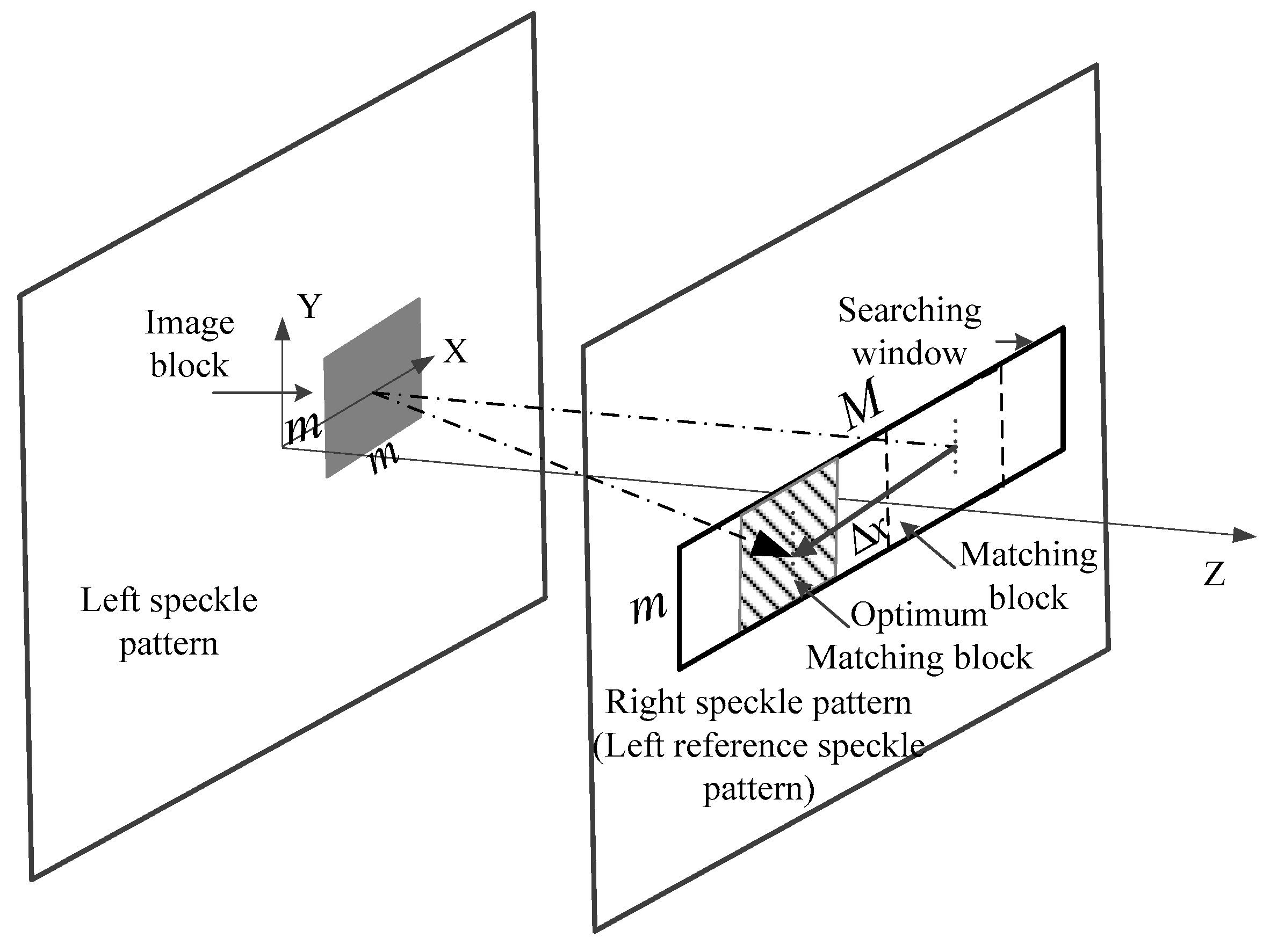
For the monocular mode, Equation (4) is employed to estimate the displacement. As shown in Figure 6, we extract a square image block (or subset) of size from the left speckle pattern. Due to the position of the image sensors and the laser projector, the block matching algorithm is confined along the X-axis only. Thus, a search window of size from the left reference speckle pattern is extracted, and the central pixel of the image block and the searching window share the same Y coordinates. The m parameters are odd numbers, and . Then the full-search block-matching method and the correlation Equation (6) are used to find the optimum matching block and estimate the displacement of the center pixel of the image block. Finally, we use Equation (3) to convert the displacement to .
For the binocular mode, the baseline length is twice that of the monocular mode; therefore, the deformation is larger and needs to be considered. In the matching process, Equation (5) is employed to estimate the displacement. The parameter is set as 0, and is set as –3/8, 0, 3/8, respectively. We round the calculated the pixel position to extract a square block from search window. The remaining process is the same as the monocular mode and then we acquire the displacement for the center pixel of the image block.
Step 6: The integration of two displacements and the depth mapping.
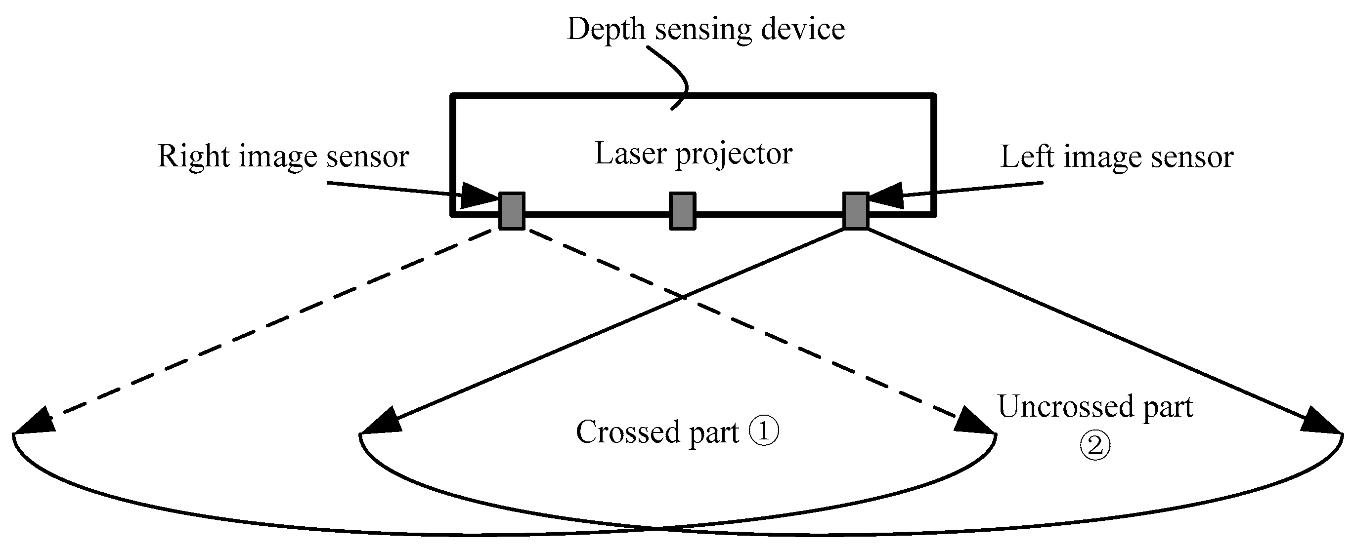
As shown in Figure 7, the field of view (FoV) of the left image sensor can be divided into two parts. One is the field of the crossed part, the other is the uncrossed part. For the pixel in the crossed part, if , then is selected as the final displacement , otherwise we compare the maximum correlation coefficients of the two matching modes and the larger one is selected as the final displacement . For the pixel in the uncrossed part, we cannot obtain the displacement , therefore, the is selected as the final displacement .
Based on the obtained the final displacement , we can calculate the distance information for the target object by triangulation according to Equation (1).
Step 7: Obtain the depth map.
Move the center pixel of the image block to the next neighboring pixel in the same row, and repeat steps 5 and 6 to obtain distance information for the neighboring pixel. Then the whole depth image can be obtained on the pixel-by-pixel and line-by-line basis.
4. Hardware Architecture and Implementation
In this paper, our method is implemented on a hardware platform. Figure 8 shows the architecture of our depth-sensing method. There are three main modules in the FPGA, i.e., consistency enhancement, shadow detection, and disparity estimation, and two external modules, the microcontroller unit (MCU) and flash memory. On the one hand, the MCU controls the reading and writing of the flash memory. Before processing, the reference image needs to be solidified in flash memory in advance, so the MCU will send a writing signal to control the flash memory through the inter-integrated circuit (I2C) bus. In the processing stage, the FPGA reads the reference data from flash memory; thus, the writing signal needs to be changed as a reading signal. On the other hand, there are some thresholds in our method, such as the in the consistency enhancement and the threshold in the displacements integration step. The MCU help us to adjust these thresholds outside the FPGA.
The pipeline framework is the heart of the hardware implementation. For example, the input image is scanned from the upper-left pixel to the lower-right pixel to generate a fixed data stream. However, every pixel is processed with the surrounding pixels in steps 3, 4 and 5. Then the block extraction submodule is essential in the three main modules. As show in Figure 9, the line buffers and D-trigger are used in this submodule to extract a image block. The length of the line buffer is equal to the image width and each D-trigger represents a clock cycle delay. The extraction of the searching window also uses the same architecture, except the length of the D-trigger is changed to .
In consistency enhancement module, after the block extraction module, there is an average submodule to calculate the average gray value of the extracted image block. Then comparator and multiplier are employed to enhance the central pixel according to Equation (7). In the shadow detection module, the comparator and counter are employed for the extracted image block to detect whether the central pixel is in the shadow area.
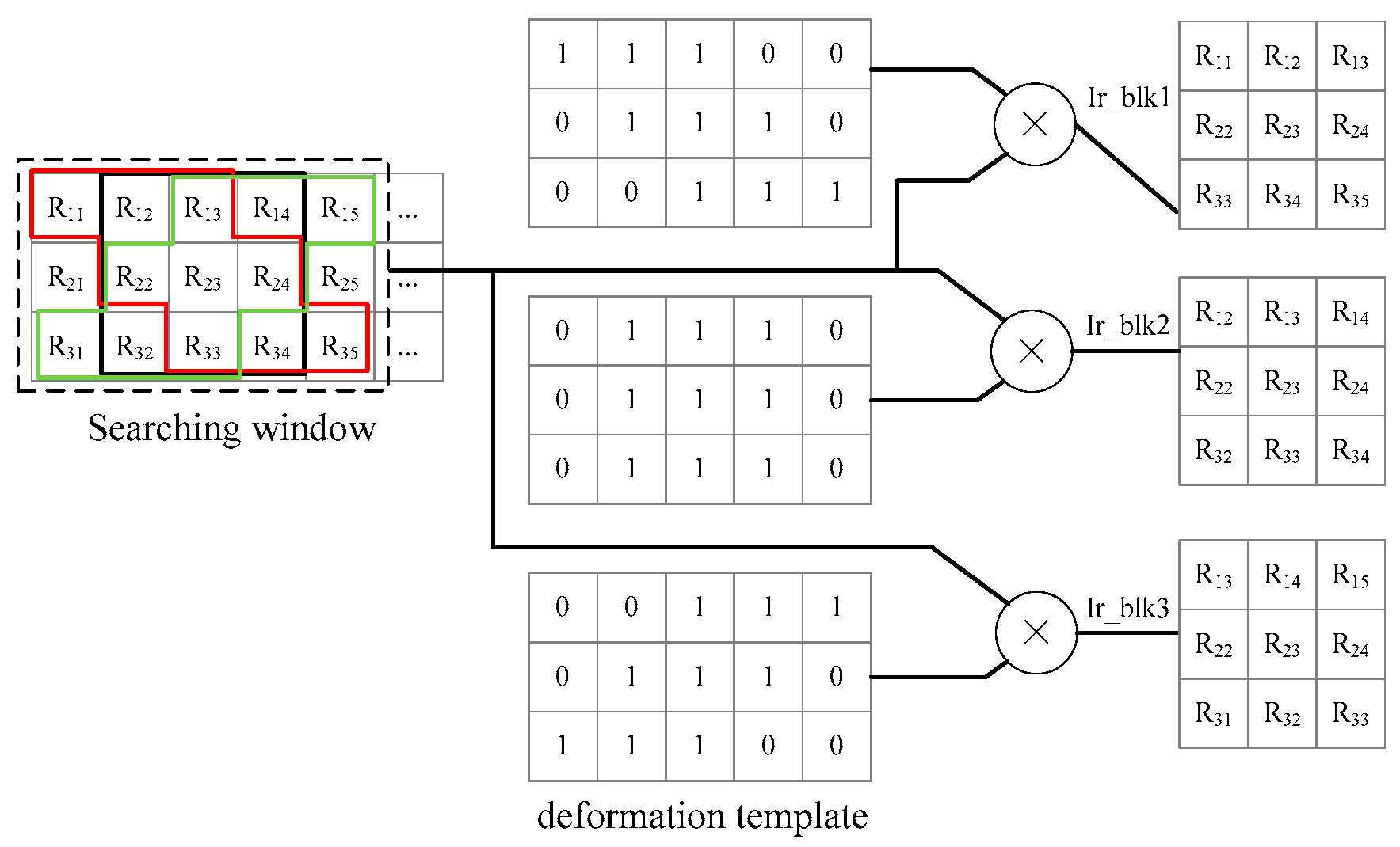
In disparity estimation, after the extraction of the image block and the searching window, the matching blocks in the searching window and image block are fed into the correlation submodule to calculate the correlation coefficients according to Equation (6). Then, the max submodule selects the max coefficient and acquires the corresponding displacement. However, there is a slight difference in the binocular mode because the deformation is considered in our paper. The matching block extraction contains an extra submodule, i.e., the deformation block extraction submodule, and an example for this submodule is given in Figure 10 by and , . For every central pixel in the searching window, we extract three matching blocks marked in red, black, and green. The deformation templates have been stored in advanced. Then a block with central pixel is multiplied with the three templates. If the pixel in the template is one, the corresponding pixel in the block will be retained to form the matching block.
For the last two submodules, displacement conversion and triangulation, we establish two lookup tables (LUTs), which store the calculating results in ROM, according to Equations (1) and (3) in Section 2.1, respectively. Every input displacement corresponds to a register address, and the result is read from the corresponding address.
5. Experimental Results and Discussion
We designed an FPGA hardware platform, as shown in Figure 11, to verify the depth sensing algorithm proposed in this paper. On the platform, we use the near-infrared laser projector (emitting laser speckle pattern), similar to that used in Kinect and two identical IR image sensors (receiving the laser speckle pattern, with output resolution supporting 1280 × 960 at 60 Hz), which are fixed on an aluminum plate. Our proposed depth-sensing method is verified on an Altera FPGA (type: EP4CE115F23C8N, Intel Corporation, Santa Clara, CA, USA).
5.1. The Validation of the Transforming Relationship between Two Displacements
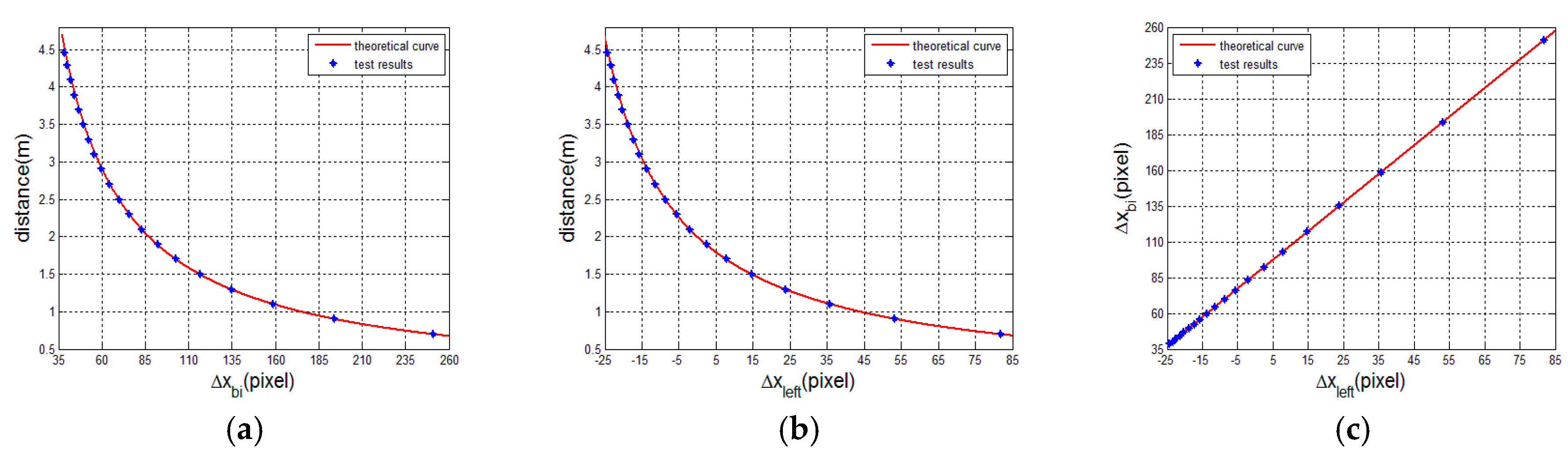
In this part, we validate the transforming relationship between the two displacements and from two matching modes. We capture a set of left and right speckle patterns projected on a standard plane that is perpendicular to the optical axis (Z-axis) of the laser projector and parallel to the left reference speckle pattern plane. The distance information of every speckle pattern is known, and the range is from 0.7 m to 4.46 m. The tested displacements and for each pattern are estimated and listed in Table 1 and Table 2. In the two tables, the theoretical displacements calculated from Equations (1) and (2) are also listed, where the related camera parameters , , the baseline , and . From Table 1 and Table 2, it can be found that the error of is slightly larger than that of . The reason is that the baseline of the binocular mode is twice the length of that of the monocular mode. For displacements , from 0.7 to 2.5 m, the error of the test value decreases with the increase in distance. After 2.5 m, the error fluctuation is stable between 0.47 and 0.61. For displacements , the error of the test value around the reference distance is at a minimum and the error between the theoretical and test values is no more than one pixel. In Figure 12, we plot the ranging curves calculated from Equations (1) and (2) and the transforming curve from Equation (3) and, additionally, the test displacements are also plotted and represented, shown as blue plots. It intuitively shows that all of the blue plots are basically on the red line.
5.2. The Spatial Resolution in X-Y Direction
In this paper, we divide the speckle pattern into blocks (or subsets) to estimate the disparity of every pixel. According to the triangulation principle, the spatial resolution in the X-Y direction is proportional to the size of the divided block and is inversely proportional to distance. The relationship can be expressed as
where represents the block size. In our method, reducing the size of the matching block is performed to improve the spatial resolution of the depth map, but it will reduce the matching accuracy. Therefore, we analyze the error rate of different sizes of blocks at different distances to select the appropriate block size. The two matching modes are performed from 0.7 to 4.46 with block sizes of 25 × 25 and 17 × 17, and and represent the estimated displacements, respectively. In the experimental results, we find that, with the larger block size of 25 × 25, there are no mismatching pixels in the two matching modes. Then, when the smaller block size of 17 × 17 is used, for every pixel, if , we assume that the matching result is an error. Table 3 lists the error rate of the two matching modes with the block size of 17 × 17. The results show that almost no mismatching appears in binocular mode before 3.5 m and the error rate is also very low from 3.7 m to 4.1 m. Therefore, the 17 × 17 block can be selected to perform the DIC algorithm. Moreover, it is obvious that, in monocular mode, the matching results are very fine around the reference distance; in other distances, the mismatching appears—especially at 0.7 m, the mismatching is very serious. In addition, the main calculation is performed in the disparity estimation step (step 5). Although the two matching modes are performed in the present method, we adopt the smaller block without the increase of the calculation amount in comparison to the 25 × 25 block size.
5.3. The Analysis and Comparison of Results
Firstly, we employ our method to test people based on our hardware platform and the results are shown in Figure 13. Figure 13a is the output depth image from the monocular mode, with some mismatching happening on the finger part, as shown in the green circle. Figure 13b is the output depth image from the binocular mode, in which the fingers are clearer. However, the occluded areas marked by red curves impact the quality of the whole image. Thus, we correct the occluded areas through Figure 13a to generate the final depth image, as shown in Figure 13c. Comparing Figure 13a with Figure 13b, it is clear that the recognition ability of the monocular mode for tiny objects is lower than that of the binocular mode and mismatching is easier to appear on the similar objects in monocular mode after reducing the block size. Conversely, the noise on the body is slightly greater in Figure 13b. The reason is that the surface of the body is relatively complex. The occlusion also exists on the surface. The black area around the person is the detected shadow area and the final result (Figure 13c) proves that our method can primarily integrate the advantage of Figure 13a,b.
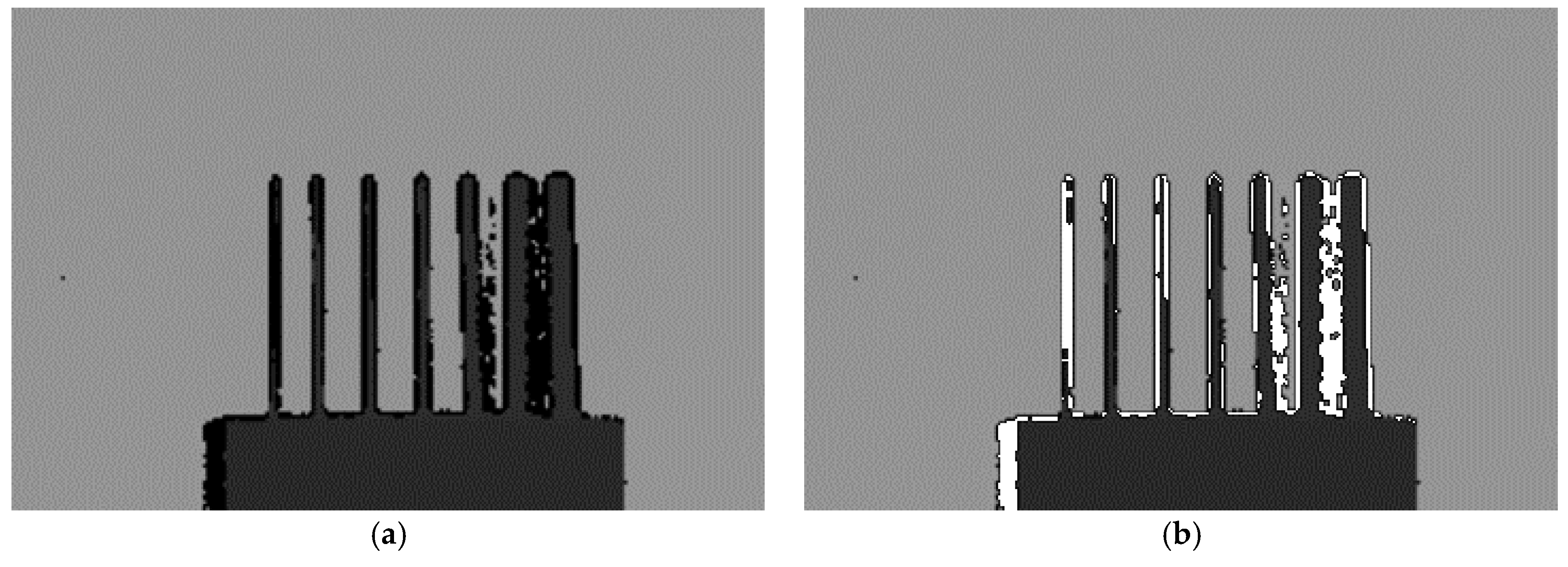
In order to test the spatial resolution of our system and intuitively compare the results with other similarly devices, such as the Xtion Pro, Kinect, Kinect 2, and Realsense R200, the depth maps on the several straight sticks with known width, as shown in Figure 14, are obtained and shown in Figure 15. The widths of the straight sticks are 5, 8, 10, 12, 15, 20, and 25 mm, from left to right. As shown in Figure 15, the results from our method are always better than that from the Kinect, Xtion Pro and Realsense. For example, it is obvious that the first stick still can be better identified at a testing distance of 1.5 m in Figure 15f, but it only can be identified at 0.7 m in Figure 15b,c,e. At 1.9 m, there are still six sticks in our depth map, but only three sticks in other three maps. Moreover, it is obvious that the noise in Figure 15e is great and the depth map on the flat object always flickers. The reason is that Intel sacrifices the performance of the Realsense in order to reduce the dimensions. The dimensions of the RealSense R200 are only 101.56 (length) × 9.55 (height) × 3.8 (width), which is the smallest depth sensor at present. Compared with the Kinect 2, our results is slightly better before 1.5 , because the Kinect 2 cannot identify the first stick at 1.5 m. Beyond the testing distance of 1.5 m, our method smooths the depth of the thinner sticks that cannot be tested. However, the Kinect 2 can mark these uncertain areas, although it also cannot obtain the depth value of these objects, such as the location of the first stick from 1.5 m to 3.1 m. Although there are some problems in our method, the results from Figure 13 and Figure 15 still prove that the present method not only improves the spatial resolution of the depth image, but also ensures the quality of depth image.
In Figure 15, we simplify the tested scene and objects, measuring the spatial resolution of different devices under an ideal circumstance. The results are optimal to a large extent. In practical applications, the scenes and structure of objects are complicated, and the tested results will be affected. Therefore, in the following, we presented more experimental results and discussed them.
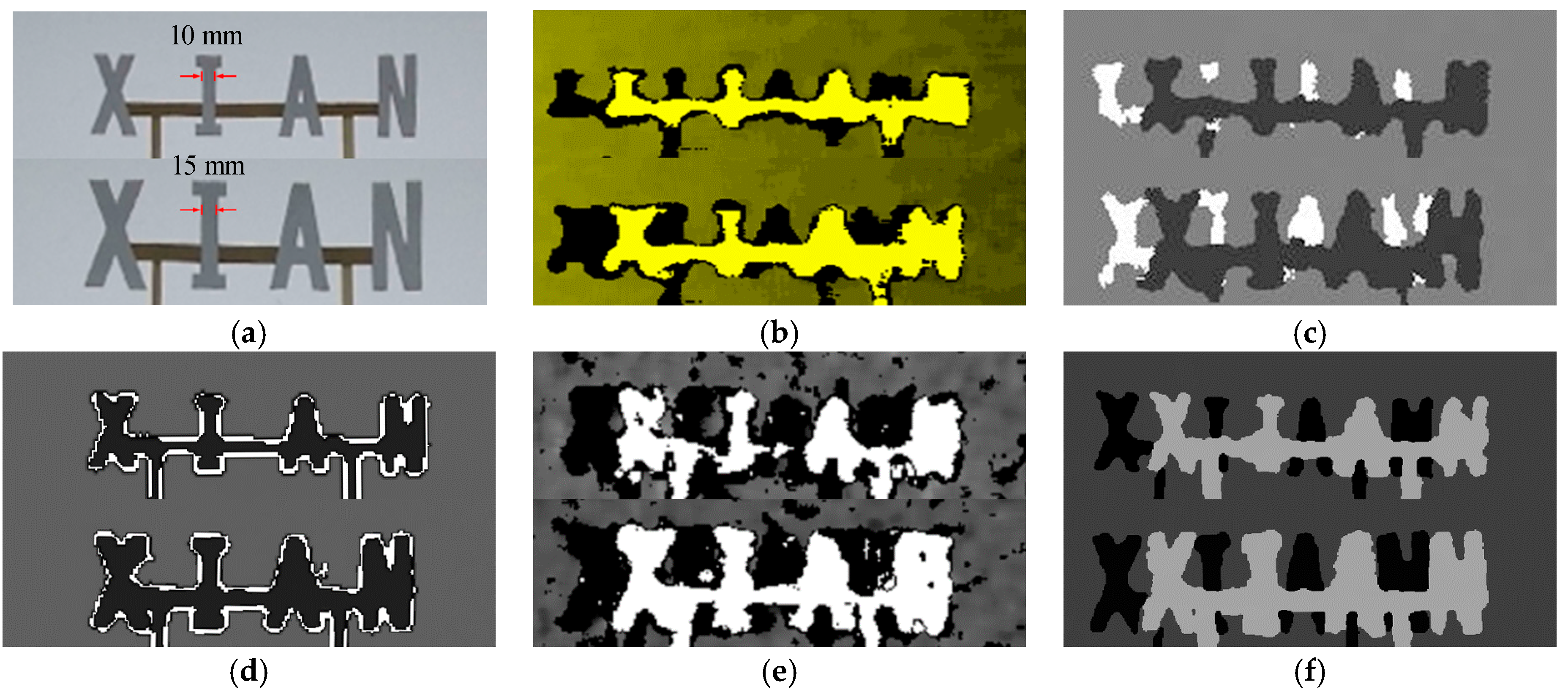
As shown in Figure 16, we tried our system on some capital letters. The strokes are 10 mm (the upper line) and 15 mm (the lower line), respectively, which have been labeled in Figure 16a. The testing distance is about 1.15 m. In Figure 14 and Figure 15, sticks with the width of 10 mm and 15 mm are the third and fifth ones, respectively. It can be concluded that the two sticks can be tested by these depth sensing devices at 1.15 m. The test results in Figure 16 are consistent with this conclusion. All devices can detect that there are some objects at this position. However, it is different to accurately recognize which letters they are. For example, for the letter “N,” in Figure 16b,c,e, the test results in the upper line are poor. In the lower line, the results in Figure 16b,c slightly improve, but they look more like the letter “H.” Figure 16d,f show an improvement over the other three, but there are also problems in the test results. The holes in the letter “A” are not detected by our system or Kinect 2.
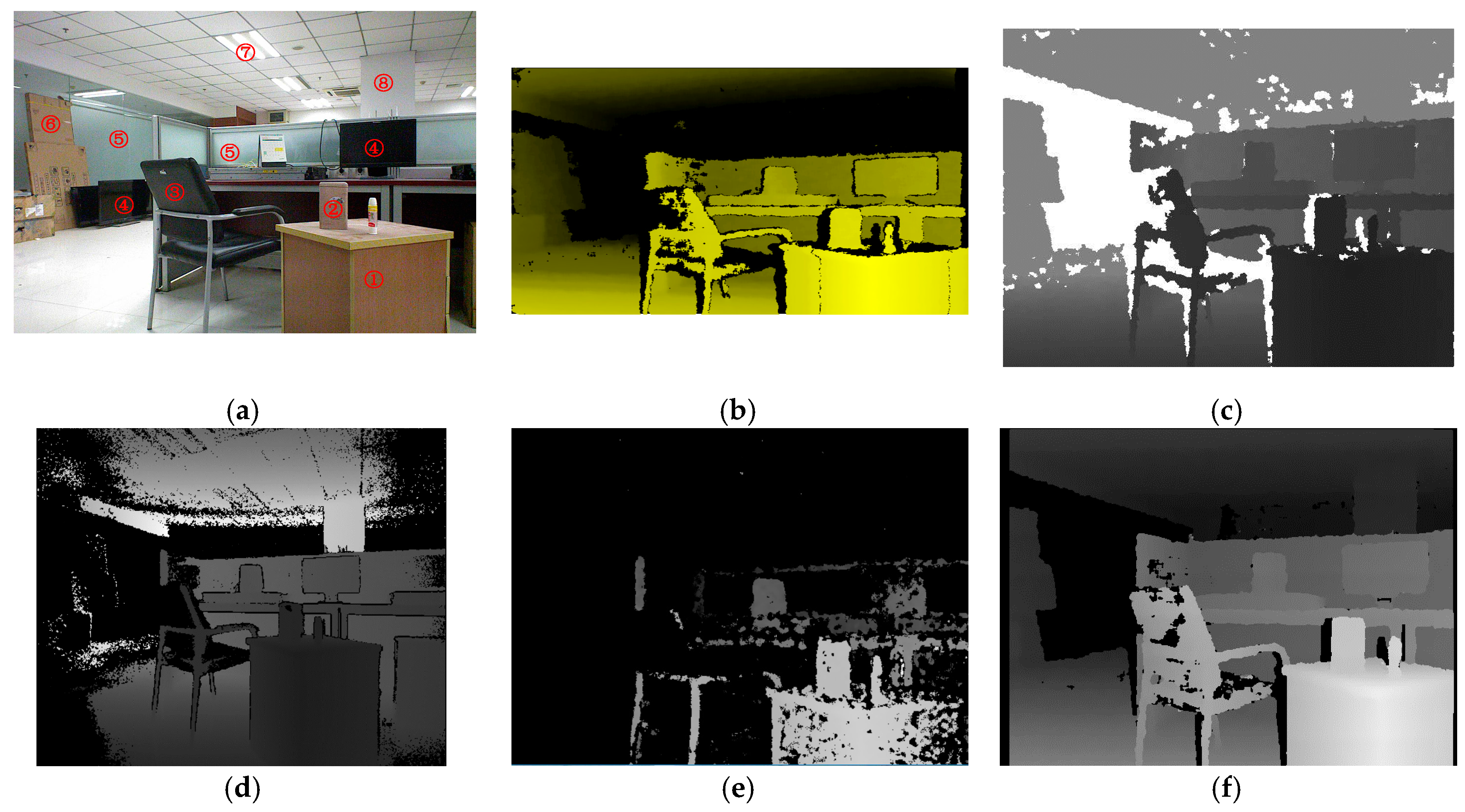
At last, we performed an experiment in a complex scene with furniture and present the results here in Figure 17. Table 4 shows the working mode and performance features of every device. The Xtion and Kinect employ the same chip (Primesense P1080), and the performance features are almost the same, so we do not list them in this table. Firstly, from Figure 17, we can see that the depth capture distance of our system and Kinect 2 is obviously an improvement over the other devices. Only Object ⑧ can be tested in Figure 17d,f. Secondly, the Kinect 2 adopts ToF technology, while other devices are all based on structured light. Object ⑥ can be tested in Figure 17b,c,f. However, Kinect 2 cannot be detected it in its range limit. Therefore, we consider that sometimes the structured-light technology is better than the ToF technology. Finally, the optical phenomena will affect the measurement results. In Figure 17d, there are some noises on Object ②, which is a mirror reflection object. The surface of Object ③ absorbs the light, which significantly affects the performance of the depth measurement based on active vision.
6. Conclusions
In this paper, an FPGA hardware design method for a depth sensing system based on active structured light is presented to improve the spatial resolution of the depth image with two infrared cameras. Firstly, the infrared cameras, based on narrow band-pass filtering, cooperate with the infrared laser to capture the clearer speckle pattern, which is projected by laser and used to mark the space. Secondly, we improved the spatial resolution in the X-Y direction by reducing the size of the matching block, but the smaller size reduces the matching strain precision. Thus, the two matching modes are combined to obtain more precise data. Moreover, the method solves the occlusion problem existing in traditional binocular stereo systems. Thirdly, we introduce the full pipeline architecture of the depth sensing method and verified it on an FPGA platform. However, if our system is to be widely adopted in the future, some optimization is needed to limit hardware resources and power consumption, and more and various scenes are also needed to verify the system; this will be the focus of our future work.
Acknowledgments
This work was supported by the National Natural Science Foundation of China under Grant No. 61571358 and No. 61627811; and Shaanxi Industrial Science and Technology Project under Grant No. 2015GY058.
Author Contributions
Chenyang Ge and Nanning Zheng provided the initial idea of this research. Huimin Yao and Chenyang Ge performed the experiments and wrote the paper. Jianru Xue and Nanning Zheng provided valuable advice in the experiments and manuscript writing.
Conflicts of Interest
The authors declare no conflict of interest.
Appendix A
In the depth images from the Kinect 2 in Figure 15d, the uncertain areas in the depth images are marked by dark pixels. This makes the depth of the measured sticks difficult to be distinguished from the uncertain area. Therefore, we made a small change in Figure 15d, as shown in Figure A1b; the uncertain areas are marked by white pixels.
Figure A1.
Depth images at distance 1.5 m from Kinect 2: (a) original depth image; (b) revised depth image.
Figure A1.
Depth images at distance 1.5 m from Kinect 2: (a) original depth image; (b) revised depth image.
References
- Zhang, Z. Microsoft kinect sensor and its effect. IEEE Multimedia 2012, 19, 4–10. [Google Scholar] [CrossRef]
- Han, J.; Shao, L.; Xu, D.; Shotton, J. Enhanced computer vision with microsoft kinect sensor: A review. IEEE Trans. Cybern. 2013, 43, 1318–1334. [Google Scholar] [PubMed]
- Iii, F.A.M.; Lauder, A.; Rector, K.; Keeling, P.; Cherones, A.L. Measurement of active shoulder motion using the Kinect, a commercially available infrared position detection system. J. Shoulder Elbow Surg. Am. Shoulder Elbow Surg. 2015, 25, 216–223. [Google Scholar]
- Hernandez-Belmonte, U.H.; Ayala-Ramirez, V. Real-time hand posture recognition for human-robot interaction tasks. Sensors 2016, 16, 36. [Google Scholar] [CrossRef] [PubMed]
- Plouffe, G.; Cretu, A. Static and dynamic hand gesture recognition in depth data using dynamic time warping. IEEE Trans. Instrum. Meas. 2016, 65, 305–316. [Google Scholar] [CrossRef]
- Kondyli, A.; Sisiopiku, V.P.; Zhao, L.; Barmpoutis, A. Computer assisted analysis of drivers’ body activity using a range camera. IEEE Intell. Transp. Syst. Mag. 2015, 7, 18–28. [Google Scholar] [CrossRef]
- Yue, H.; Chen, W.; Wu, X.; Wang, J. Extension of an iterative closest point algorithm for simultaneous localization and mapping in corridor environments. J. Electron. Imaging 2016, 25, 023015. [Google Scholar] [CrossRef]
- Kim, H.; Lee, S.; Kim, Y.; Lee, S.; Lee, D.; Ju, J.; Myung, H. Weighted joint-based human behavior recognition algorithm using only depth information for low-cost intelligent video-surveillance system. Expert Syst. Appl. 2015, 45, 131–141. [Google Scholar] [CrossRef]
- Izadi, S.; Kim, D.; Hilliges, O.; Molyneaux, D.; Newcombe, R.; Kohli, P.; Shotton, J.; Hodges, S.; Freeman, D.; Davison, A. Kinect fusion: Real-time 3D reconstruction and interaction using a moving depth camera. In Proceedings of the ACM Symposium on User Interface Software and Technology, Santa Barbara, CA, USA, 16–19 October 2011; pp. 559–568. [Google Scholar]
- Tang, S.; Zhu, Q.; Chen, W.; Darwish, W.; Wu, B.; Hu, H.; Chen, M. enhanced RGB-D mapping method for detailed 3D indoor and outdoor modeling. Sensors 2016, 16, 1589. [Google Scholar] [CrossRef] [PubMed]
- Jin, S.; Cho, J.; Pham, X.D.; Lee, K.M.; Park, S.K.; Kim, M.; Jeon, J.W. FPGA design and implementation of a real-time stereo vision system. IEEE Trans. Circuits Syst. Video Technol. 2010, 20, 15–26. [Google Scholar]
- Banz, C.; Hesselbarth, S.; Flatt, H.; Blume, H.; Pirsch, P. Real-time stereo vision system using semi-global matching disparity estimation: Architecture and FPGA-implementation. In Proceedings of the International Conference on Embedded Computer Systems, Samos, Greece, 19–22 July 2010; pp. 93–101. [Google Scholar]
- Geng, J. Structured-light 3D surface imaging: a tutorial. Adv. Opt. Photonics 2011, 3, 128–160. [Google Scholar] [CrossRef]
- Salvi, J.; Pagès, J.; Batlle, J. Pattern codification strategies in structured light systems. Pattern Recognit. 2004, 37, 827–849. [Google Scholar] [CrossRef]
- Kim, W.; Wang, Y.; Ovsiannikov, I.; Lee, S.H.; Park, Y.; Chung, C.; Fossum, E. A 1.5Mpixel RGBZ CMOS image sensor for simultaneous color and range image capture. In Proceedings of the IEEE International Solid-state Circuits Conference Digest of Technical Papers, San Francisco, CA, USA, 19–23 February 2012; pp. 392–394. [Google Scholar]
- Sarbolandi, H.; Lefloch, D.; Kolb, A. Kinect range sensing: Structured-light versus time-of-flight kinect. Comput. Vision Image Underst. 2015, 139, 1–20. [Google Scholar] [CrossRef]
- Gere, D.S. Depth Perception Device and System. U.S. Patent 2013/0027548, 31 January 2013. [Google Scholar]
- Lin, B.S.; Su, M.J.; Cheng, P.H.; Tseng, P.J.; Chen, S.J. Temporal and spatial denoising of depth maps. Sensors 2015, 15, 18506–185025. [Google Scholar] [CrossRef] [PubMed]
- Camplani, M.; Salgado, L. Efficient spatio-temporal hole filling strategy for Kinect depth maps. In Proceedings of the IS&T/SPIE Electronic Imaging, Burlingame, CA, USA, 22–26 January 2012. [Google Scholar]
- Yao, H.; Ge, C.; Hua, G.; Zheng, N. The VLSI implementation of a high-resolution depth-sensing SoC based on active structured light. Mach. Vision Appl. 2015, 26, 533–548. [Google Scholar] [CrossRef]
- Ma, S.; Shen, Y.; Qian, J.; Chen, H.; Hao, Z.; Yang, L. Binocular Structured Light Stereo Matching Approach for Dense Facial Disparity Map; Springer: Berlin/Heidelberg, Germany, 2011; pp. 550–559. [Google Scholar]
- An, D.; Woodward, A.; Delmas, P.; Chen, C.Y. Comparison of Structured Lighting Techniques with a View for Facial Reconstruction. 2012. Available online: https://www.researchgate.net/publication/268427066_Comparison_of_Structured_Lighting_Techniques_with_a_View_for_Facial_Reconstruction (accessed on 3 March 2017).
- Nguyen, T.T.; Slaughter, D.C.; Max, N.; Maloof, J.N.; Sinha, N. Structured light-based 3D reconstruction system for plants. Sensors 2015, 15, 18587–18612. [Google Scholar] [CrossRef] [PubMed]
- Yang, R.; Cheng, S.; Yang, W.; Chen, Y. Robust and accurate surface measurement using structured light. IEEE Trans. Instrum. Meas. 2008, 57, 1275–1280. [Google Scholar] [CrossRef]
- Dekiff, M.; Berssenbrügge, P.; Kemper, B.; Denz, C.; Dirksen, D. Three-dimensional data acquisition by digital correlation of projected speckle patterns. Appl. Phys. B 2010, 99, 449–456. [Google Scholar] [CrossRef]
- Robert, L.; Nazaret, F.; Cutard, T.; Orteu, J.J. Use of 3-D digital image correlation to characterize the mechanical behavior of a fiber reinforced refractory castable. Exp. Mech. 2007, 47, 761–773. [Google Scholar] [CrossRef]
- Lu, H.; Cary, P.D. Deformation measurements by digital image correlation: Implementation of a second-order displacement gradient. Exp. Mech. 2000, 40, 393–400. [Google Scholar] [CrossRef]
- Hirschmüller, H. Stereo processing by semiglobal matching and mutual information. IEEE Trans. Pattern Anal. Mach. Intell. 2008, 30, 328–341. [Google Scholar] [CrossRef] [PubMed]
- Scharstein, D.; Szeliski, R. A taxonomy and evaluation of dense two-frame stereo correspondence algorithms. Int. J. Comput. Vision 2002, 47, 7–42. [Google Scholar] [CrossRef]
Figure 1.
Front view of the experiment platform.
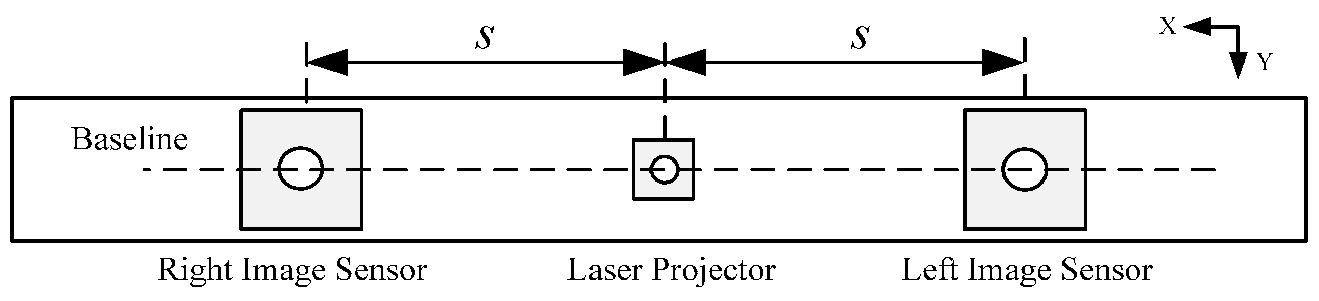
Figure 2.
Schematic diagram of the triangulation principle.

Figure 3.
Flow diagram of depth-sensing method.
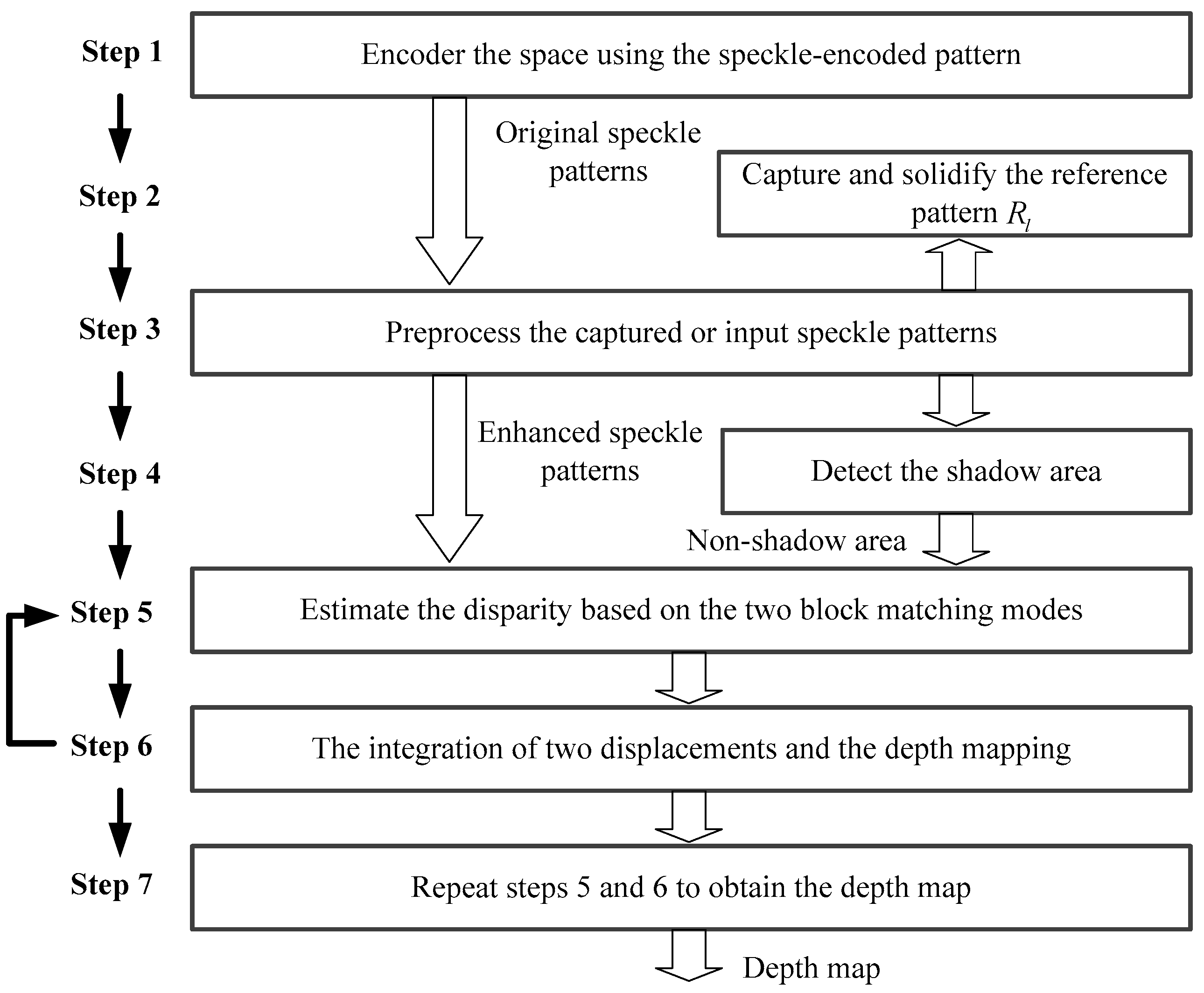
Figure 4.
Schematic diagram of the principle of shadow formation.

Figure 5.
The speckle pattern and the results after preprocessing: (a) the speckle pattern; (b) the consistency enhancement result; and (c) the shadow detection result.
Figure 5.
The speckle pattern and the results after preprocessing: (a) the speckle pattern; (b) the consistency enhancement result; and (c) the shadow detection result.
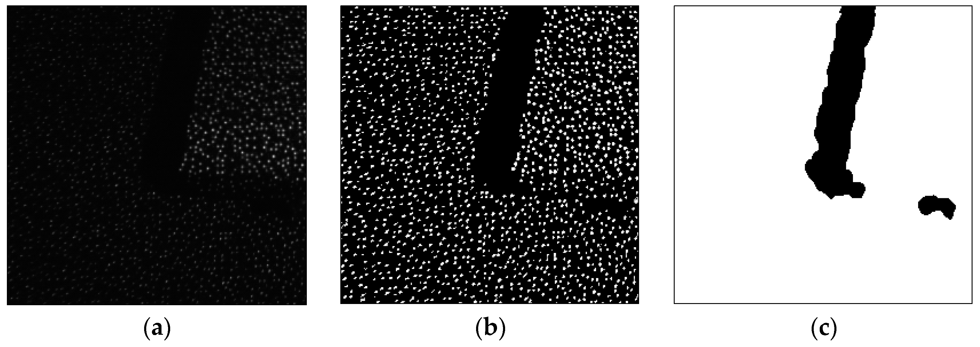
Figure 6.
Schematic diagram of the block-matching-based disparity estimation.

Figure 7.
The field of view (FoV) of the output depth image about the two working modes.

Figure 8.
Architecture of the depth sensing method.
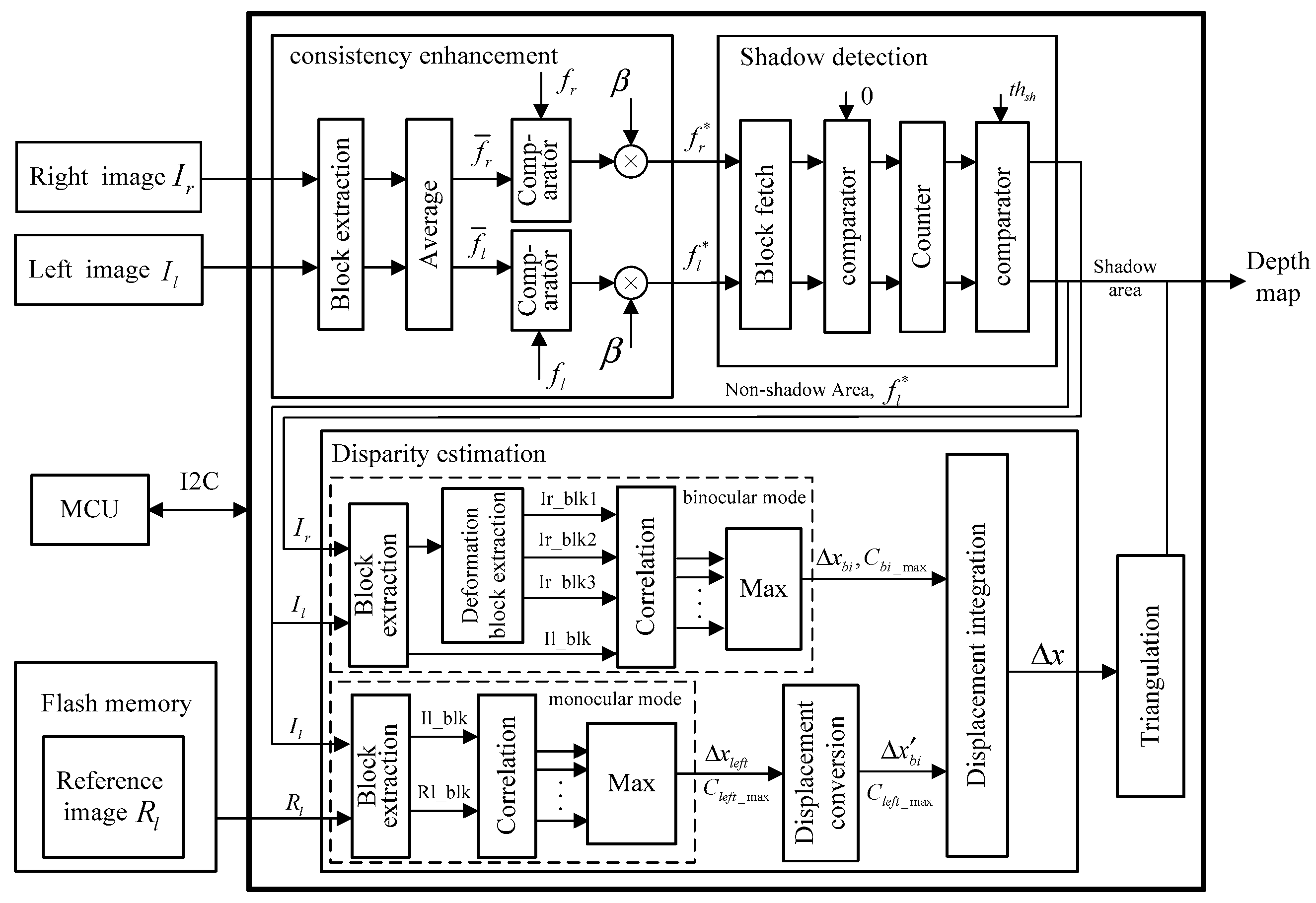
Figure 9.
Block extraction submodule.
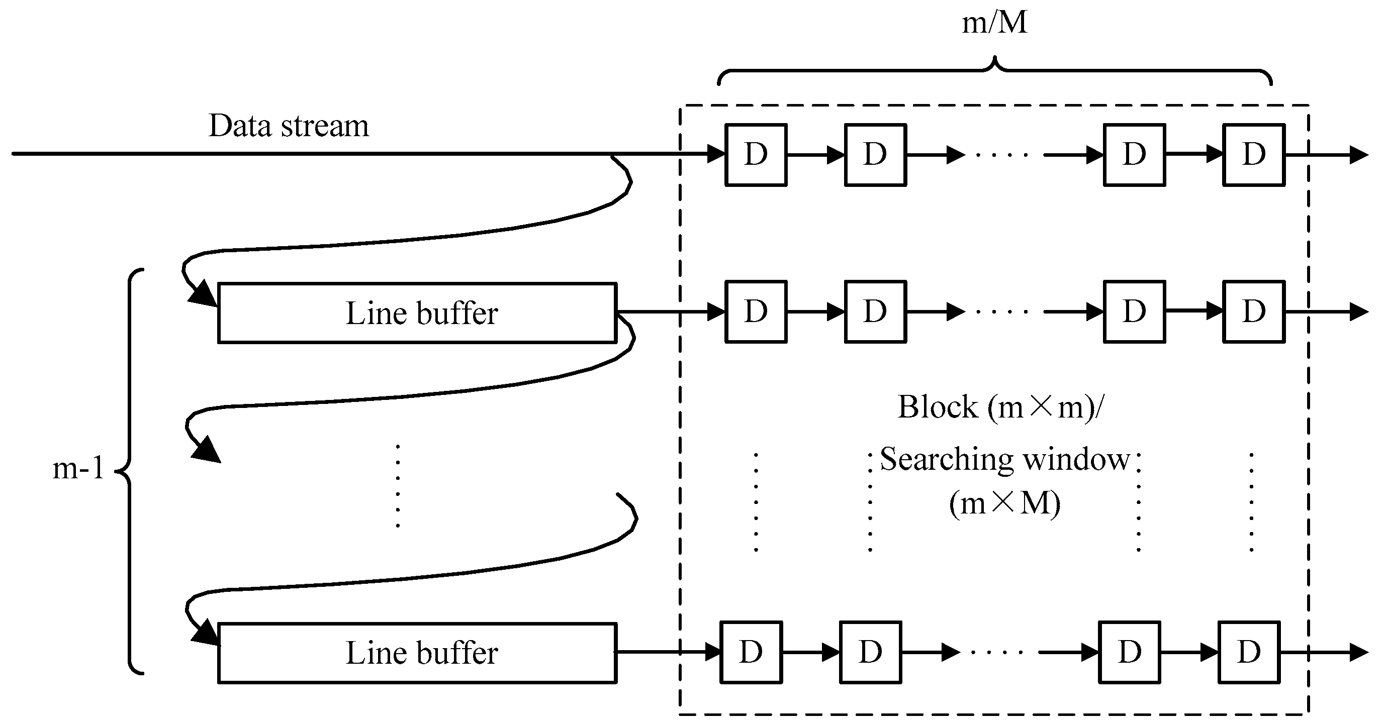
Figure 10.
Deformation block extraction submodule.

Figure 11.
The hardware test platform.
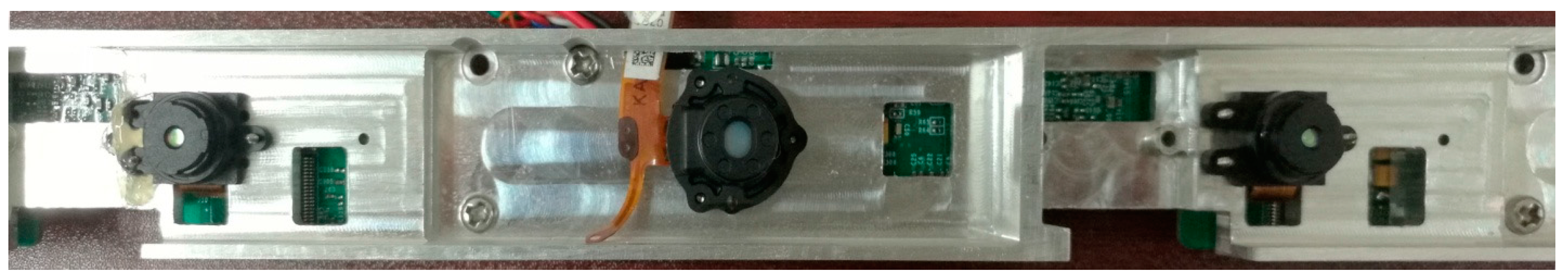
Figure 12.
The test results and theoretical curves from Equations (1), (2), and (3). (a) The distance curve of displacements ; (b) the distance curve of displacements ; (c) the transforming curve between displacements and .
Figure 12.
The test results and theoretical curves from Equations (1), (2), and (3). (a) The distance curve of displacements ; (b) the distance curve of displacements ; (c) the transforming curve between displacements and .

Figure 13.
The depth image (a) from monocular mode (b) from binocular mode (c) from the combination of the two matching modes.
Figure 13.
The depth image (a) from monocular mode (b) from binocular mode (c) from the combination of the two matching modes.
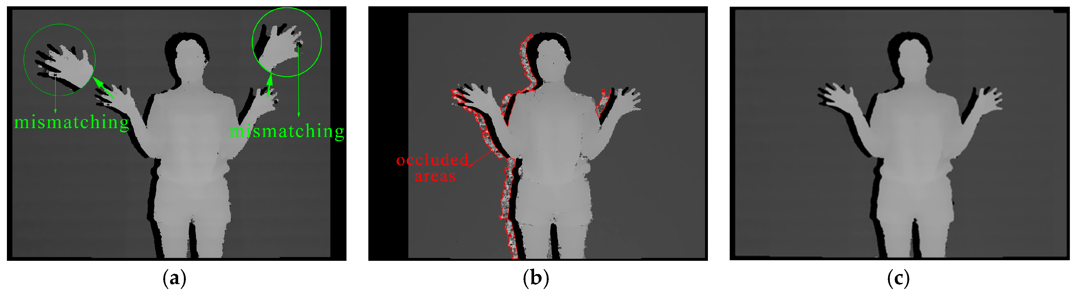
Figure 14.
The width of the straight sticks.
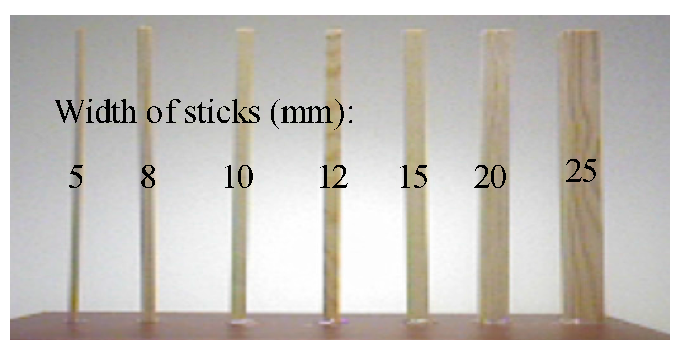
Figure 15.
The different widths of the straight sticks (5, 8, 10, 12, 15, 20, and 25 mm from left to right) at different distances. (a) Color image; (b) Xtion Pro; (c) Kinect; (d) Kinect 2 (see Appendix A for more details); (e) Realsense R200; (f) our method.
Figure 15.
The different widths of the straight sticks (5, 8, 10, 12, 15, 20, and 25 mm from left to right) at different distances. (a) Color image; (b) Xtion Pro; (c) Kinect; (d) Kinect 2 (see Appendix A for more details); (e) Realsense R200; (f) our method.
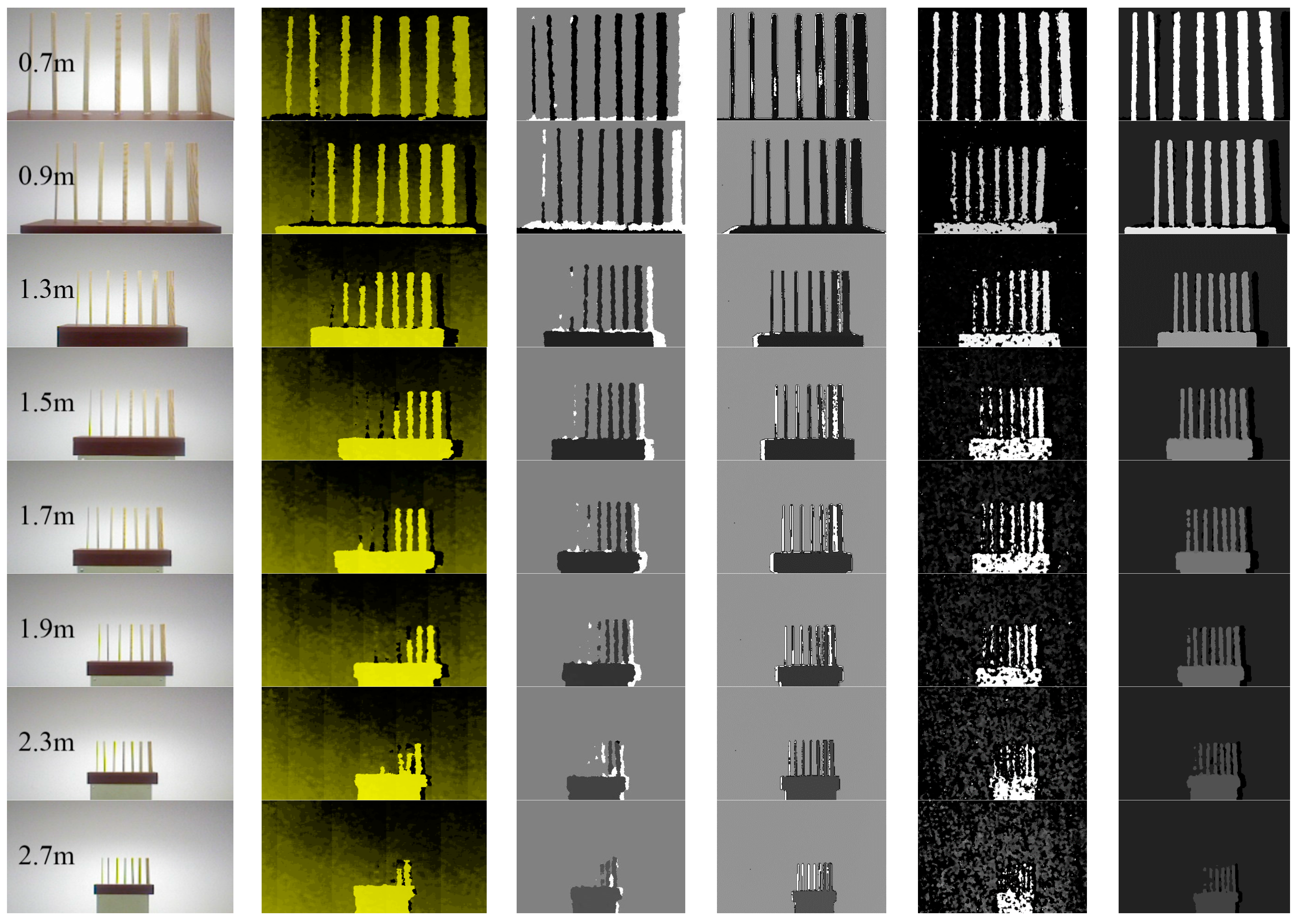
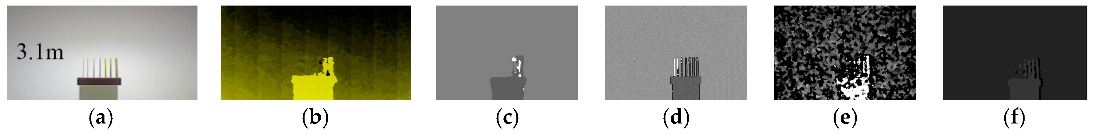
Figure 16.
The test results on some capital letters. (a) Color image; (b) Xtion Pro; (c) Kinect; (d) Kinect 2 (see Appendix A for more details); (e) Realsense R200; (f) our method.
Figure 16.
The test results on some capital letters. (a) Color image; (b) Xtion Pro; (c) Kinect; (d) Kinect 2 (see Appendix A for more details); (e) Realsense R200; (f) our method.

Figure 17.
The test results in the complex scene with furniture. (a) Color image; (b) Xtion Pro; (c) Kinect; (d) Kinect 2; (e) Realsense R200; (f) our method.
Figure 17.
The test results in the complex scene with furniture. (a) Color image; (b) Xtion Pro; (c) Kinect; (d) Kinect 2; (e) Realsense R200; (f) our method.


Table 1.
A list of the displacements at different distance.
| Distance(m) | Theory Value | Test Value | Distance(m) | Theory Value | Test Value |
|---|---|---|---|---|---|
| 0.7 | 250.06 | 250.79 ± 0.94 | 2.7 | 64.67 | 64.21 ± 0.51 |
| 0.9 | 193.08 | 193.66 ± 0.75 | 2.9 | 60.08 | 59.60 ± 0.59 |
| 1.1 | 157.96 | 158.58 ± 0.71 | 3.1 | 56.21 | 55.71 ± 0.57 |
| 1.3 | 134.26 | 135.05 ± 0.74 | 3.3 | 52.88 | 52.35 ± 0.63 |
| 1.5 | 116.36 | 116.83 ± 0.65 | 3.5 | 49.91 | 49.33 ± 0.58 |
| 1.7 | 102.55 | 102.73 ± 0.61 | 3.7 | 47.19 | 46.62 ± 0.58 |
| 1.9 | 92.06 | 92.06 ± 0.53 | 3.9 | 44.80 | 44.24 ± 0.61 |
| 2.1 | 83.12 | 83.15 ± 0.56 | 4.1 | 42.61 | 42.02 ± 0.47 |
| 2.3 | 75.76 | 75.70 ± 0.53 | 4.3 | 40.64 | 40.04 ± 0.50 |
| 2.5 | 70.07 | 69.99 ± 0.50 | 4.46 | 39.11 | 38.45 ± 0.58 |
Table 2.
A list of the displacements at different distance.
| Distance(m) | Theory Value | Test Value | Distance(m) | Theory Value | Test Value |
|---|---|---|---|---|---|
| 0.7 | 81.40 | 81.79 ± 0.67 | 2.7 | −11.30 | −11.37 ± 0.80 |
| 0.9 | 52.90 | 53.20 ± 0.59 | 2.9 | −13.59 | −13.75 ± 0.58 |
| 1.1 | 35.34 | 35.64 ± 0.58 | 3.1 | −15.53 | −15.67 ± 0.43 |
| 1.3 | 23.50 | 23.87 ± 0.58 | 3.3 | −17.20 | −17.36 ± 0.43 |
| 1.5 | 14.55 | 14.75 ± 0.47 | 3.5 | −18.68 | −18.89 ± 0.42 |
| 1.7 | 7.64 | 7.73 ± 0.32 | 3.7 | −20.04 | −20.22 ± 0.37 |
| 1.9 | 2.39 | 2.41 ± 0.28 | 3.9 | −21.24 | −21.37 ± 0.44 |
| 2.1 | −2.08 | −2.09 ± 0.30 | 4.1 | −22.33 | −22.49 ± 0.50 |
| 2.3 | −5.76 | −5.69 ± 0.51 | 4.3 | −23.32 | −23.45 ± 0.45 |
| 2.5 | −8.60 | −8.72 ± 0.68 | 4.46 | −24.08 | −24.28 ± 0.50 |
Table 3.
The error rate (‰) of the two matching modes at different distance.
| Distance (m) | Binocular Mode | Monocular Mode | Distance (m) | Binocular Mode | Monocular Mode |
|---|---|---|---|---|---|
| 0.7 | 0 | 0.48 | 2.7 | 0 | 0.03 |
| 0.9 | 0 | 0.22 | 2.9 | 0 | 0.03 |
| 1.1 | 0 | 0.18 | 3.1 | 0 | 0.04 |
| 1.3 | 0 | 0.06 | 3.3 | 0 | 0.03 |
| 1.5 | 0 | 0 | 3.5 | 0 | 0.08 |
| 1.7 | 0 | 0 | 3.7 | 0.01 | 0.07 |
| 1.9 | 0 | 0 | 3.9 | 0.01 | 0.06 |
| 2.1 | 0 | 0 | 4.1 | 0.03 | 0.06 |
| 2.3 | 0 | 0 | 4.3 | 0.09 | 0.06 |
| 2.5 | 0 | 0 | 4.46 | 0.20 | 0.09 |
Table 4.
The performance comparison.
| Item | Kinect | Kinect 2 | Realsense R200 | Our Method |
|---|---|---|---|---|
| Working mode | Structured light | ToF | Structured light | Structured light |
| Range limit | 0.8~3.5 m | 0.5~4.5 m | 0.4~2.8 m | 0.8~4.5 m |
| Framerate | 30 fps | 30 fps | Up to 60 fps | Up to 60 fps |
| Image resolution | 640 × 480 | 512 × 424 | Up to 640 × 480 | Up to 1280 × 960 |
| Bits of depth image | 10bits | unpublished | 12bits | 12bits |
| Vertical Field | 43° | 60° | 46° ± 5° | 43° |
| Horizontal Field | 57° | 70° | 59° ± 5° | 58° |
| Output interface | USB 2.0 | USB 3.0 | USB 3.0 | USB 3.0 |
© 2017 by the authors. Licensee MDPI, Basel, Switzerland. This article is an open access article distributed under the terms and conditions of the Creative Commons Attribution (CC BY) license (http://creativecommons.org/licenses/by/4.0/).
Share and Cite
MDPI and ACS Style
Yao, H.; Ge, C.; Xue, J.; Zheng, N. A High Spatial Resolution Depth Sensing Method Based on Binocular Structured Light. Sensors 2017, 17, 805. https://doi.org/10.3390/s17040805
AMA Style
Yao H, Ge C, Xue J, Zheng N. A High Spatial Resolution Depth Sensing Method Based on Binocular Structured Light. Sensors. 2017; 17(4):805. https://doi.org/10.3390/s17040805
Chicago/Turabian StyleYao, Huimin, Chenyang Ge, Jianru Xue, and Nanning Zheng. 2017. "A High Spatial Resolution Depth Sensing Method Based on Binocular Structured Light" Sensors 17, no. 4: 805. https://doi.org/10.3390/s17040805
Note that from the first issue of 2016, this journal uses article numbers instead of page numbers. See further details here.