
A Comprehensive Analysis on Wearable Acceleration Sensors in Human Activity Recognition


Abstract
:1. Introduction
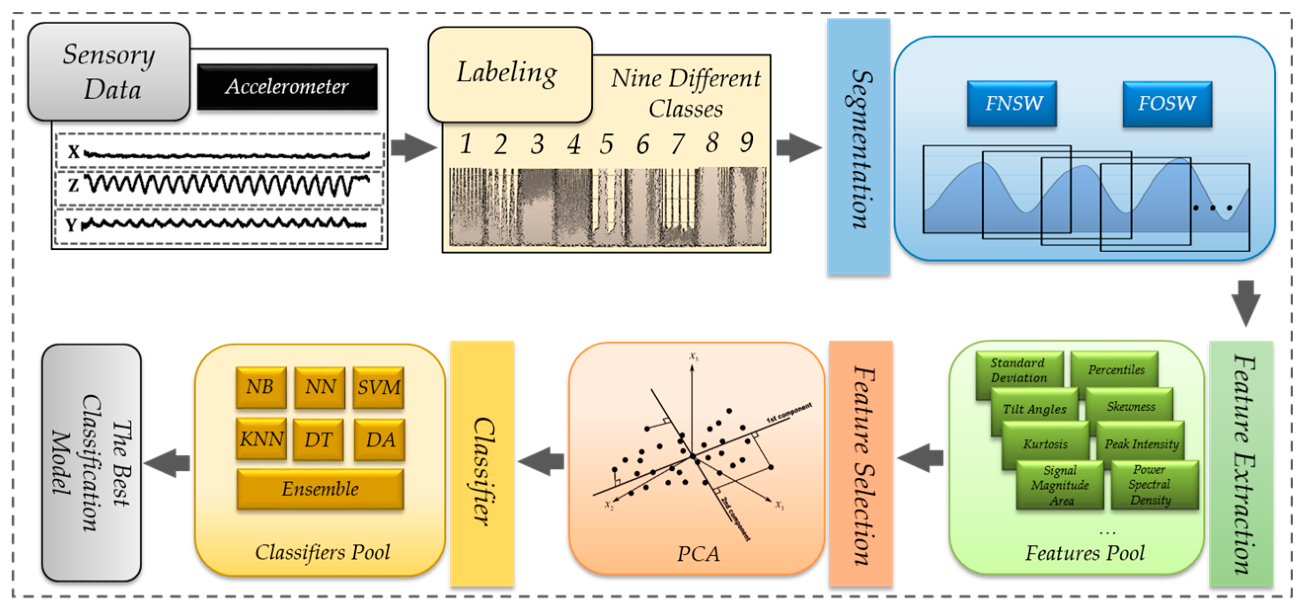
2. Backgrounds and Methodologies
2.1. Data Segmentation, Feature Extraction and Selection
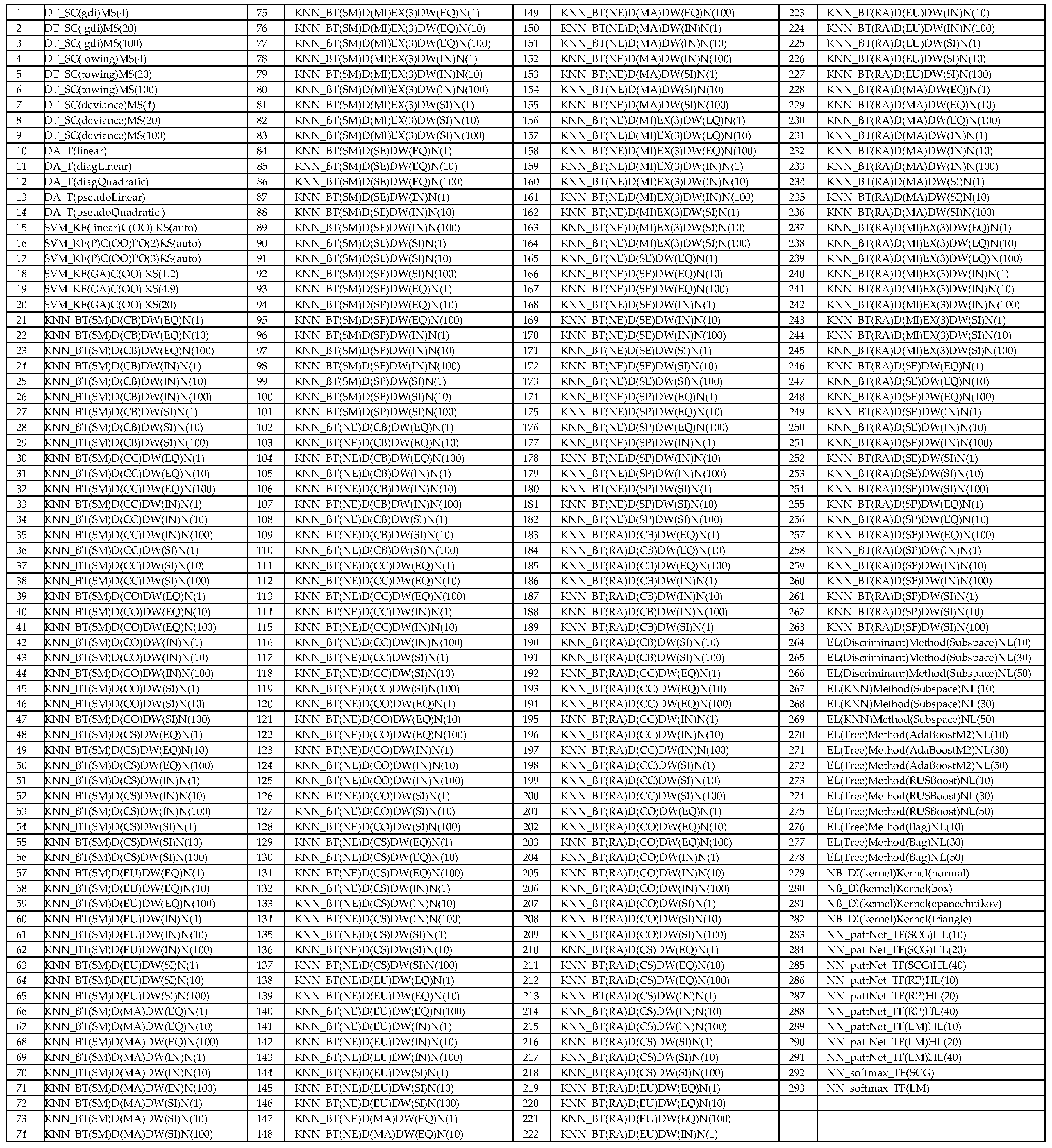
2.2. Machine Learning Techniques
3. Datasets
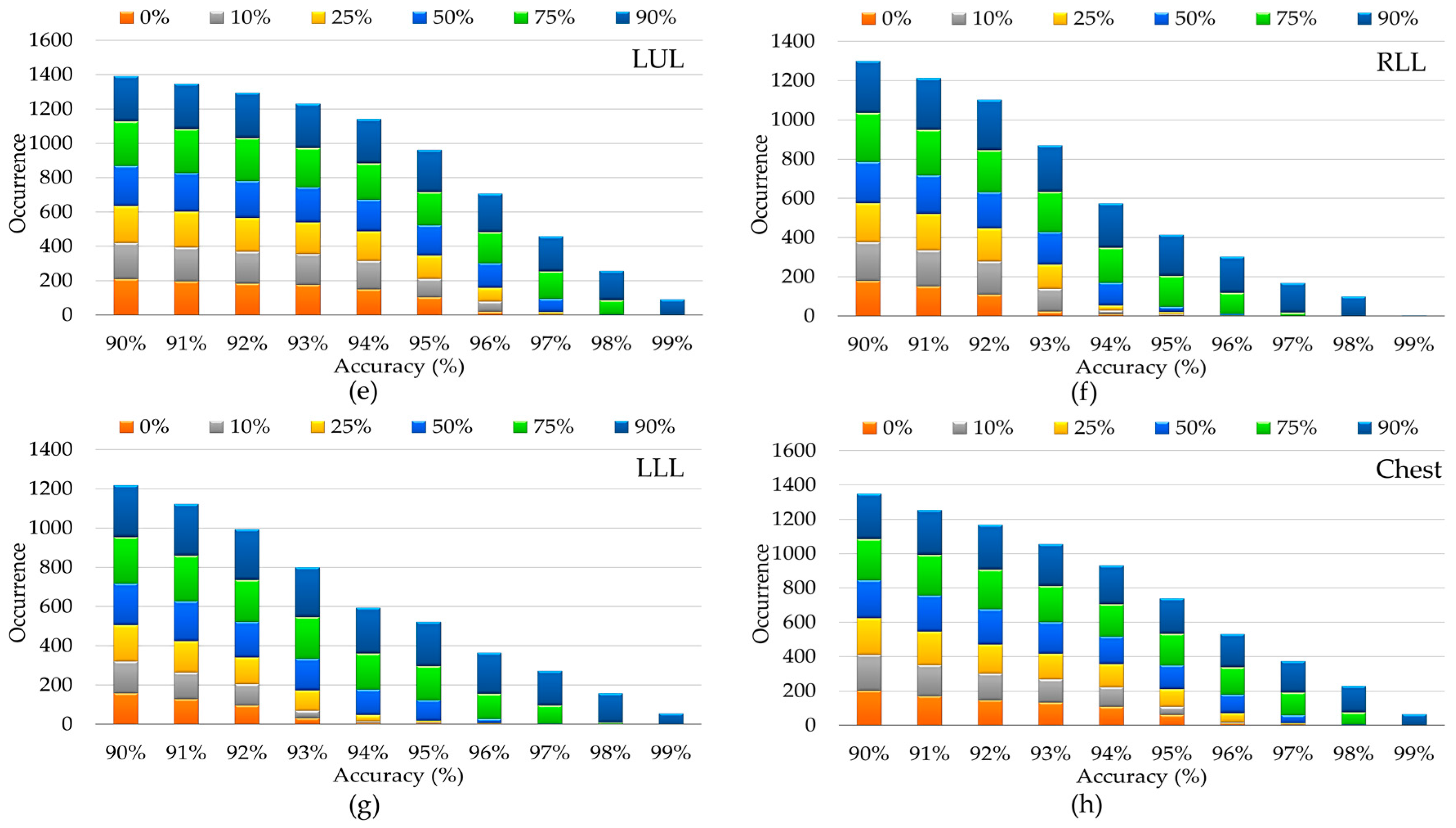
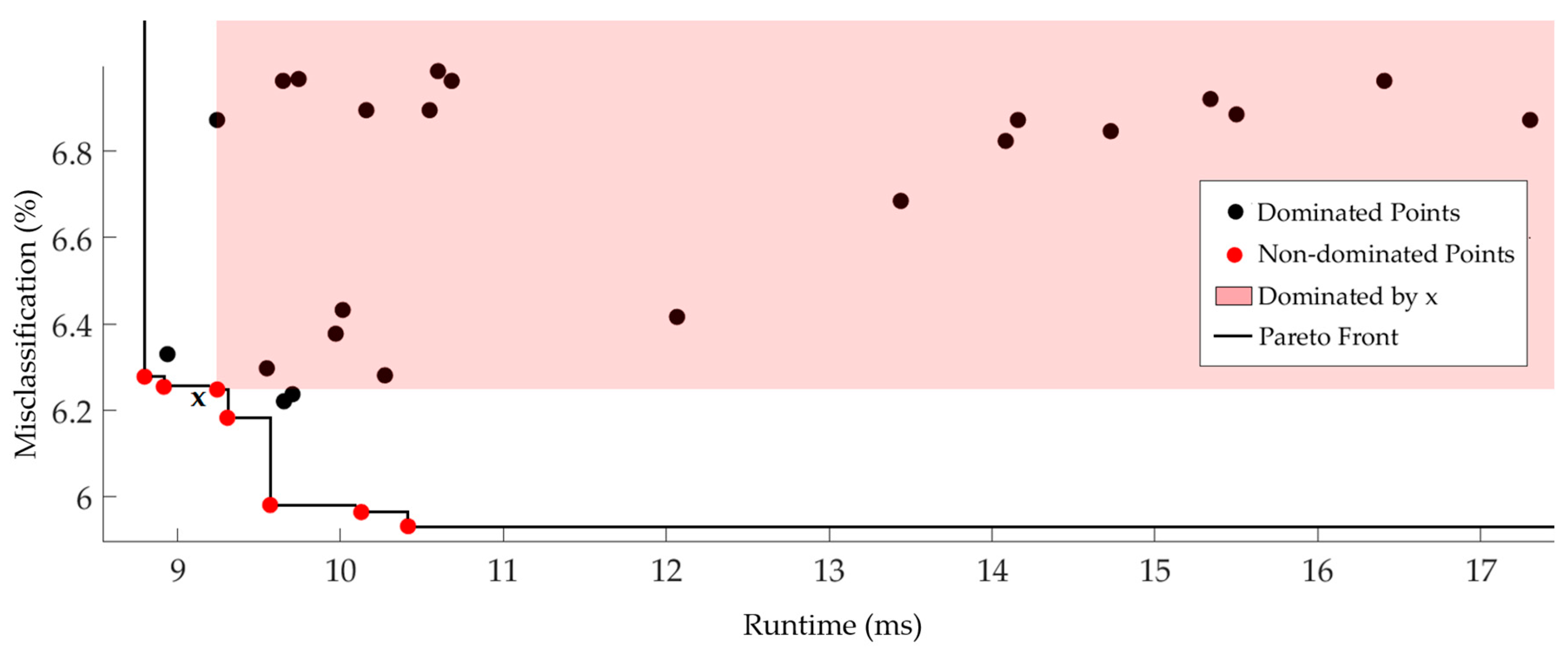
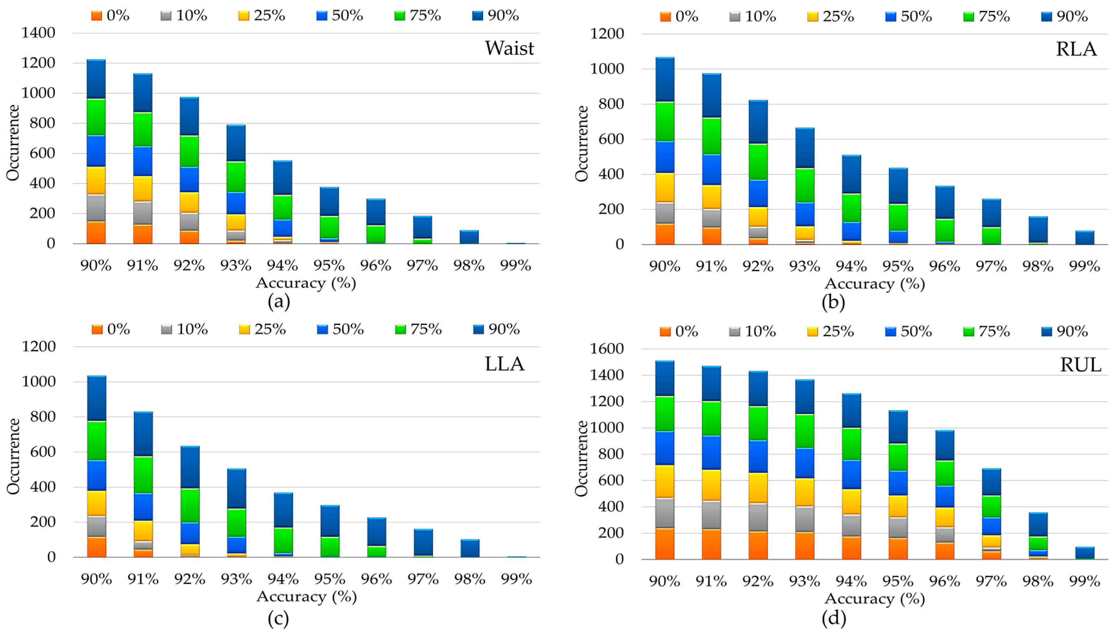
4. Experimental Results and Discussions
5. Conclusions
Author Contributions
Conflicts of Interest
Abbreviations
Appendix A
Appendix A.1. Decision Tree
Appendix A.2. Discriminant Analysis

| Split Criterion | Description | Split Criterion | Description | Split Criterion | Description | |
|---|---|---|---|---|---|---|
| Gini’s Diversity Index (GDI) | Deviance | Towing rule | ||||
| Let L(i)/R(i) denote the fraction of members of class i in the left/right child node after a split and p(L)/p(R) are the fractions of observations that split to the left/right | ||||||
| p(i) is the probability that an arbitrary sample belongs to class li. | based the concept of entropy from information theory |
Appendix A.3. Support Vector Machine
| Kernel | Formula | Kernel | Formula | Kernel | Formula |
|---|---|---|---|---|---|
| Linear | Polynomial | Radial basis function (RBF) |
| Distance Metric | Description | Distance Metric | Description | Distance Metric | Description |
|---|---|---|---|---|---|
| Euclidean | Standardized Euclidean | is the standard deviation of the and over the sample set | Correlation | and | |
| City Block | Minkowski | In this work, p = 3 | Mahalanobis | C is the covariance matrix | |
| Chebychev | Cosine | Spearman | is the rank of over If any values are tied, their average rank is computed |
Appendix A.4. K-Nearest Neighbors
Appendix A.5. Ensemble Methods
Appendix A.6. Naïve Bayes
| Kernel Type | Formula | Kernel Type | Formula |
|---|---|---|---|
| Uniform | Epanechnikov | ||
| Normal (Gaussian) | Triangular |
Appendix A.7. Neural Network

References
- Kumar, S.; Nilsen, W.; Pavel, M.; Srivastava, M. Mobile health: Revolutionizing healthcare through transdisciplinary research. IEEE Comput. 2013, 46, 28–35. [Google Scholar] [CrossRef]
- Khusainov, R.; Azzi, D.; Achumba, I.; Bersch, S. Real-Time Human Ambulation, Activity, and Physiological Monitoring: Taxonomy of Issues, Techniques, Applications, Challenges and Limitations. Sensors 2013, 13, 12852–12902. [Google Scholar] [CrossRef] [PubMed] [Green Version]
- Chen, L.; Hoey, J.; Nugent, C.D.; Cook, D.J.; Yu, Z. Sensor-Based Activity Recognition. IEEE Trans. Syst. Man Cybern. Part C: Appl. Rev. 2012, 42, 790–808. [Google Scholar] [CrossRef]
- He, Z.; Jin, L. Activity recognition from acceleration data using AR model representation and SVM. In Proceedings of the 2008 International Conference on Machine Learning and Cybernetics, Kunming, China, 12–15 July 2008; Volume 4, pp. 2245–2250.
- Anguita, D.; Ghio, A.; Oneto, L.; Parra, X.; Reyes-Ortiz, J.L. A Public Domain Dataset for Human Activity Recognition Using Smartphones. In Proceedings of the 21th European Symposium on Artificial Neural Network. Computational Intelligence and Machine Learning (ESANN 2013), Bruges, Belgium, 24–26 April 2013.
- Ugulino, W.; Cardador, D.; Vega, K.; Velloso, E.; Milidiu, R.; Fuks, H. Wearable Computing: Accelerometers’ Data Classification of Body Postures and Movements. In Advances in Artificial Intelligence—SBIA 2012, Proceedings of the 21st Brazilian Symposium on Artificial Intelligence, Curitiba, Brazil, 20–25 October 2012; Springer: Berlin/Heidelberg, Germany, 2012; pp. 52–61. [Google Scholar]
- Lara, O.D.; Labrador, M.A. A Survey on Human Activity Recognition using Wearable Sensors. IEEE Commun. Surv. Tutor. 2013, 15, 1192–1209. [Google Scholar] [CrossRef]
- Banos, O.; Galvez, J.-M.; Damas, M.; Pomares, H.; Rojas, I. Window Size Impact in Human Activity Recognition. Sensors 2014, 14, 6474–6499. [Google Scholar] [CrossRef] [PubMed]
- Preece, S.J.; Goulermas, J.Y.; Kenney, L.P.; Howard, D.; Meijer, K.; Crompton, R. Activity identification using body-mounted sensors—A review of classification techniques. Physiol. Meas. 2009, 30, 4. [Google Scholar] [CrossRef] [PubMed]
- Igual, R.; Medrano, C.; Plaza, I. A comparison of public datasets for acceleration-based fall detection. Med. Eng. Phys. 2015, 37, 870–878. [Google Scholar] [CrossRef] [PubMed]
- Stisen, A.; Blunck, H.; Bhattacharya, S.; Prentow, T.; Kjrgaard, M.; Dey, A.; Sonne, T.; Jensen, M. Smart devices are different: Assessing and mitigating mobile sensing heterogeneities for activity recognition. In Proceedings of the 13th ACM Conference on Embedded Networked Sensor Systems, Seoul, Korea, 1–4 November 2015; pp. 127–140.
- Blunck, H.; Bhattacharya, S.; Stisen, A.; Prentow, T.S.; Kjærgaard, M.B.; Dey, A.; Jensen, M.M.; Sonne, T. Activity recognition on smart devices: Dealing with diversity in the wild. GetMobile 2016, 20, 34–38. [Google Scholar]
- Labrador, M.A.; Lara, O.D.; Human, Y. Activity Recognition: Using Wearable Sensors and Smartphones; Chapman & Hall/CRC Computer and Information Science Series; CRC Press Book: Boca Raton, FL, USA, 2013. [Google Scholar]
- Keogh, E.; Chu, S.; Hart, D.; Pazzani, M. An Online Algorithm for Segmenting Time Series. In Proceedings of the International Conference on Data Mining, San Jose, CA, USA, 29 November–2 December 2001; pp. 289–296.
- Janidarmian, M.; Radecka, K.; Zilic, Z. Automated diagnosis of knee pathology using sensory data. In Proceedings of the IEEE/EAI International Conference on Wireless Mobile Communication and Healthcare (Mobihealth), Athens, Greece, 3–5 November 2014; pp. 95–98.
- Krishnan, N.C.; Juillard, C.; Colbry, D.; Panchanathan, S. Recognition of hand movements using wearable accelerometers. J. Ambient Intell. Smart Environ. 2009, 2, 143–155. [Google Scholar]
- Sun, L.; Zhang, D.; Li, B.; Guo, B.; Li, S. Activity Recognition on an Accelerometer Embedded Mobile Phone with Varying Positions and Orientations. In Ubiquitous Intelligence and Computing; Lecture Notes in Computer Science; Springer: Berlin/Heidelberg, Germany, 2010; Volume 6406, pp. 548–562. [Google Scholar]
- He, Z.; Jin, L. Activity recognition from acceleration data based on discrete consine transform and SVM. In Proceedings of the IEEE International Conference on Systems, Man and Cybernetics, 2009 (SMC 2009), San Antonio, TX, USA, 11–14 October 2009; pp. 5041–5044.
- Peterek, T.; Penhaker, M.; Gajdoš, P.; Dohnálek, P. Comparison of classification algorithms for physical activity recognition. In Innovations in Bio-Inspired Computing and Applications; Springer: Ostrava, Czech Republic, 2014; pp. 123–131. [Google Scholar]
- Ravi, N.; Dandekar, N.; Mysore, P.; Littman, M.L. Activity recognition from accelerometer data. In Proceedings of the 17th Conference on Innovative Applications of Artificial Intelligence (IAAI), Pittsburgh, PA, USA, 9–13 July 2005; pp. 1541–1546.
- Banos, O.; Toth, M.A.; Damas, M.; Pomares, H.; Rojas, I.; Amft, O. A benchmark dataset to evaluate sensor displacement in activity recognition. In Proceedings of the 14th International Conference on Ubiquitous Computing (Ubicomp 2012), Pittsburgh, PA, USA, 5–8 September 2012.
- Banos, O.; Villalonga, C.; Garcia, R.; Saez, A.; Damas, M.; Holgado, J.A.; Lee, S.; Pomares, H.; Rojas, I. Design, implementation and validation of a novel open framework for agile development of mobile health applications. BioMed. Eng. OnLine 2015, 14, S6. [Google Scholar] [CrossRef] [PubMed]
- Shoaib, M.; Scholten, J.; Havinga, P.J.M. Towards physical activity recognition using smartphone sensors. In Proceedings of the 10th IEEE International Conference on Ubiquitous Intelligence and Computing, Vietri sul Mare, Italy, 18–20 December 2013; pp. 80–87.
- Kwapisz, J.R.; Weiss, G.M.; Moore, S.A. Activity Recognition using Cell Phone Accelerometers. In Proceedings of the Fourth International Workshop on Knowledge Discovery from Sensor Data, Washington, DC, USA, 25 July 2010; pp. 74–82.
- Shoaib, M.; Bosch, S.; Incel, O.D.; Scholten, H.; Havinga, P.J.M. Fusion of Smartphone Motion Sensors for Physical Activity Recognition. Sensors 2014, 14, 10146–10176. [Google Scholar] [CrossRef] [PubMed]
- Janidarmian, M.; Radecka, K.; Zilic, Z. Analysis of Motion Patterns for Recognition of Human Activities. In Proceedings of the 2015 ACM 5th International Conference on Wireless Mobile Communication and Healthcare (Mobihealth), London, UK, 14–16 October 2015; pp. 68–72.
- Altun, K.; Barshan, B.; Tunçel, O. Comparative study on classifying human activities with miniature inertial and magnetic sensors. Pattern Recognit. 2010, 43, 3605–3620. [Google Scholar] [CrossRef] [Green Version]
- Liu, S.; Gao, R.X.; John, D.; Staudenmayer, J.; Freedson, P.S. SVM-based multi-sensor fusion for free-living physical activity assessment. In Proceedings of the 33rd Annual International IEEE EMBS Conference, Boston, MA, USA, 30 August–3 September 2011; pp. 3188–3191.
- Long, X.; Yin, B.; Aarts, R.M. Single-accelerometer-based daily physical activity classification. In Proceedings of the 2009 Annual International Conference of the IEEE Engineering in Medicine and Biology Society, Minneapolis, MN, USA, 3–6 September 2009; pp. 6107–6110.
- Győrbíró, N.; Fábián, Á.; Hományi, G. An activity recognition system for mobile phones. Mob. Netw. Appl. 2009, 14, 82–91. [Google Scholar] [CrossRef]
- Vahdatpour, A.; Amini, N.; Sarrafzadeh, M. On-body device localization for health and medical monitoring applications. In Proceedings of the 2011 IEEE International Conference on Pervasive Computing and Communications (PerCom), Seattle, WA, USA, 21–25 March 2011; pp. 37–44.
- Saeedi, R.; Purath, J.; Venkatasubramanian, K.; Ghasemzadeh, H. Toward seamless wearable sensing: Automatic on-body sensor localization for physical activity monitoring. In Proceedings of the 2014 36th Annual International Conference of the IEEE Engineering in Medicine and Biology Society, Chicago, IL, USA, 26–30 August 2014; pp. 5385–5388.
- Bruno, B.; Mastrogiovanni, F.; Sgorbissa, A.; Vernazza, T.; Zaccaria, R. Analysis of human behavior recognition algorithms based on acceleration data. In Proceedings of the IEEE International Conference on Robotics and Automation (ICRA), Karlsruhe, Germany, 6–10 May 2013; pp. 1602–1607.
- Casale, P.; Pujol, O.; Radeva, P. Personalization and user verification in wearable systems using biometric walking patterns. Pers. Ubiquitous Comput. 2012, 16, 563–580. [Google Scholar] [CrossRef]
- Zhang, M.; Sawchuk, A.A. USC-HAD: A Daily Activity Dataset for Ubiquitous Activity Recognition Using Wearable Sensors. In Proceedings of the ACM International Conference on Ubiquitous Computing (UbiComp) Workshop on Situation, Activity and Goal Awareness (SAGAware), Pittsburgh, PA, USA, 5–8 September 2012.
- Yang, A.; Jafari, R.; Sastry, S.; Bajcsy, R. Distributed Recognition of Human Actions Using Wearable Motion Sensor Networks. J. Ambient Intell. Smart Environ. 2009, 1, 103–115. [Google Scholar]
- Frank, K.; Röckl, M.; Vera Nadales, M.J.; Robertson, P.; Pfeifer, T. Comparison of exact static and dynamic Bayesian context inference methods for activity recognition. In Proceedings of the 8th IEEE International Conference on Pervasive Computing and Communications Workshops (PERCOM Workshops), Mannheim, Germany, 29 March–2 April 2010; pp. 189–195.
- Balaprakash, P.; Tiwari, A.; Wild, S.; Jarvis, S.A.; Wright, S.A.; Hammond, S.D. Multi objective optimization of HPC kernels for performance power and energy. In International Workshop on Performance Modeling, Benchmarking and Simulation of High Performance Computer Systems; Springer Lecture Notes in Computer Science: Denver, CO, USA, 2014; pp. 239–260. [Google Scholar]
- Fekr, A.R.; Janidarmian, M.; Radecka, K.; Zilic, Z. Respiration Disorders Classification with Informative Features for m-Health Applications. IEEE J. Biomed. Health Inform. 2016, 20, 733–747. [Google Scholar] [CrossRef] [PubMed]
- Rokach, L.; Maimon, O. Data Mining with Decision Trees: Theroy and Applications; World Scientific Publishing Co., Inc.: River Edge, NJ, USA, 2008. [Google Scholar]
- Zambon, M.; Lawrence, R.; Bunn, A.; Powell, S. Effect of alternative splitting rules on image processing using classification tree analysis. Photogramm. Eng. Remote Sens. 2006, 72, 25–30. [Google Scholar] [CrossRef]
- Theodoridis, S.; Koutroumbas, K. Pattern Recognition, 4th ed.; Elsevier/Academic Press: Cambridge, MA, USA, 2008. [Google Scholar]
- Zheng, E.; Chen, B.; Wang, X.; Huang, Y.; Wang, Q. On the Design of a Wearable Multi-sensor System for Recognizing Motion Modes and Sit-to-stand Transition. Int. J. Adv. Robot. Syst. 2014, 11, 30. [Google Scholar] [CrossRef]
- Chen, T.; Mazomenos, E.; Maharatna, K.; Dasmahapatra, S. On the trade-off of accuracy and computational complexity for classifying normal and abnormal ECG in remote CVD monitoring systems. In Proceedings on the IEEE Workshop Signal Processing Systems (SIPS), Quebec City, QC, Canada, 17–19 October 2012; pp. 37–42.
- Supervised Learning, Statistics Toolbox, MATLAB R2105b documentation. Available online: https://cn.mathworks.com/login?uri=https%3A%2F%2Fcn.mathworks.com%2Fhelp%2Freleases%2FR2015b%2Findex.html (accessed on 6 March 2017).
- Chamasemani, F.F.; Singh, Y.P. Multi-class Support Vector Machine (SVM) Classifiers—An Application in Hypothyroid Detection and Classification. In Proceedings of the 2011 Sixth International Conference on Bio-Inspired Computing: Theories and Applications (BIC-TA), Penang, Malaysia, 27–29 September 2011; pp. 351–356.
- Fekr, A.R.; Janidarmian, M.; Radecka, K.; Zilic, Z. A Medical Cloud-Based Platform for Respiration Rate Measurement and Hierarchical Classification of Breath Disorders. Sensors 2014, 14, 11204–11224. [Google Scholar] [CrossRef] [PubMed]
- Parera, J.; Angulo, C.; Rodriguez-Molinero, A.; Cabestany, J. User daily activity classification from accelerometry using feature selection and SVM. In Bio-Inspired Systems: Computational and Ambient Intelligence; LNCS: Salamanca, Spain, 2009; pp. 1137–1144. [Google Scholar]
- He, H.; Garcia, E.A. Learning from imbalanced data. IEEE Trans. Knowl. Data Eng. 2009, 21, 1263–1284. [Google Scholar]
- Dietterich, T.G.; Bakiri, G. Solving multiclass learning problem via error-correcting output codes. J. Artif. Intell. Res. 1995, 263–286. [Google Scholar]
- Foorster, K.; Monteleone, S.; Calatroni, A.; Roggen, D.; Trooster, G. Incremental KNN classifier exploiting correct—Error teacher for activity recognition. In Proceedings of the 9th International Conference on Machine Learning and Applications, Washington, DC, USA, 12–14 December 2010; pp. 445–450.
- Everitt, B.S.; Landau, S.; Leese, M.; Stahl, D. Miscellaneous Clustering Methods, in Cluster Analysis, 5th ed.; John Wiley & Sons, Ltd.: Chichester, UK, 2011. [Google Scholar]
- Hall, P.; Park, B.U.; Samworth, R.J. Choice of neighbour order in nearest-neighbour classification. Ann. Stat. 2008, 36, 2135–2152. [Google Scholar] [CrossRef]
- Anil, K.G. On optimum choice of k in nearest neighbor classification. Comput. Stat. Data Anal. 2006, 50, 3113–3123. [Google Scholar]
- Breiman, L. Bagging Predictors; Technical Report 421; Department of Statistics, University of California at Berkeley: Berkeley, CA, USA, 1994. [Google Scholar]
- Machova, K.; Barcak, F.; Bednar, P. A bagging method using decision trees in the role of base classifiers. Acta Polytech. Hung. 2006, 3, 2. [Google Scholar]
- Schapire, R.; Freund, Y. Boosting the margin: A new explanation for the effectiveness of voting methods. Ann. Stat. 1998, 26, 1651–1686. [Google Scholar] [CrossRef]
- Freund, Y.; Schapire, R.E. A Decision-Theoretic Generalization of On-Line Learning and an Application to Boosting. J. Comput. Syst. Sci. 1997, 55, 119–139. [Google Scholar] [CrossRef]
- Seiffert, C.; Khoshgoftaar, T.; Hulse, J.; Napolitano, A. RUSBoost: Improving classification performance when training data is skewed. In Proceedings of the 19th International Conference on Pattern Recognition, Tampa, FL, USA, 8–11 December 2008; pp. 1–4.
- Ho, T.K. The random subspace method for constructing decision forests. IEEE Trans. Pattern Anal. Mach. Intell. 1998, 20, 832–844. [Google Scholar]
- Bishop, C.M. Pattern Recognition and Machine Learning; Springer: Berlin, Germany, 2006. [Google Scholar]
- Lester, J.; Choudhury, T.; Kern, N.; Borriello, G.; Hannaford, B. A hybrid discriminative/generative approach for modeling human activities. In Proceedings of the 19th International Joint Conference on Artificial Intelligence, Edinburgh, UK, 30 July–5 August 2005; pp. 1541–1546.
- Cortina-Puig, M.; Istamboulie, G.; Noguer, T.; Marty, J. Analysis of Pesticide Mixtures Using Intelligent Biosensors. In Intelligent and Biosensors; Vernon, S.S., Ed.; InTech: Rijeka, Croatia, 2010; Chapter 10. [Google Scholar]
- Sharma, A.; Lee, Y.-D.; Chung, W.-Y. High Accuracy Human Activity Monitoring Using Neural Network. In Proceedings of the Third International Conference on Convergence and Hybrid Information Technology, 2008 (ICCIT ’08), Washington, DC, USA, 11–13 November 2008; Volume 1, pp. 430–435.
- Riedmiller, M.; Braun, H. A direct adaptive method for faster backpropagation learning: The RPROP algorithm. In Proceedings of the IEEE International Conference on Neural Network, San Francisco, CA, USA, 28 March–1 April 1993; pp. 586–591.
- Molier, M. A Scaled Conjugate Gradient Algorithm for Fast Supervised Learning. Neural Netw. 1993, 6, 525–533. [Google Scholar] [CrossRef]
- Hagan, M.T.; Menhaj, M. Training feed-forward networks with the Marquardt algorithm. IEEE Trans. Neural Netw. 1994, 5, 989–993. [Google Scholar] [CrossRef] [PubMed]


| Feature | Description | Feature | Description |
|---|---|---|---|
| Mean | Skewness | ||
| Minimum | Kurtosis | ||
| Maximum | Signal Power | ||
| Median | Root Mean Square | ||
| Standard Deviation | Peak Intensity | The number of signal peaks within a certain period of time | |
| Coefficients of Variation | Pearson's Correlation Coefficient | ||
| Peak-to-peak Amplitude | Inter-axis Cross-Correlation | ||
| Percentiles | Autocorrelation | ; the height of the first and second peaks and the position of the second peak of | |
| k = integer part of t; f = fractional part of t | |||
| Interquartile Range | Trapezoidal Numerical Integration | using Multiple Segment Trapezoidal Rule | |
| Pitch Angle | Signal Magnitude Area | ||
| Roll Angle | Signal Vector Magnitude | ||
| Median Crossings | t = s − | Power Spectral Density | f denotes the fth Fourier coefficient in the frequency domain; the positions and power levels of highest 6 peaks of PSD computed over the sliding window; total power in 5 adjacent and pre-defined frequency bands. |
| sgn(a,b) = {1 if (a.b) < 0; 0 if (a.b) > 0} |
| Dataset | Number of Subjects | Sensor Type | Frequency | Sensor Placement | Activity Type | Description |
|---|---|---|---|---|---|---|
| (1) [5] | 30 (19–48 year) | accelerometer gyroscope (Samsung Galaxy S II smartphone) | 50 Hz | waist (1) | walking, ascending stairs, descending stairs, sitting, standing, laying (6) | In the first trial, each subject placed the smartphone in a predetermined position i.e., the left side of the belt. However, in the second attempt, they could fix the phone in a desired position on the waist. |
| (2) [6] | 4 (28–75 year) (45 ) | ADXL335 accelerometer (connected to an ATmega328V microcontroller) | ~8 Hz | waist, left thigh, right ankle, right arm (4) | walking, sitting, sitting down, standing, standing up (5) | The data have been collected during 8 h of five different activities for all subjects. |
| (3) [27] | 8 (20–30 year) | accelerometer gyroscope magnetometer (Xsens MTx unit) | 25 Hz | chest, right and left wrists, right side of the right knee, left side of the left knee (5) | walking in a parking lot, sitting, standing, lying, ascending/descending stairs, walking on a treadmill with a speed of 4 km/h (in flat and 15° inclined positions), etc. (19) | The subjects performed nineteen activities by their own style and were not controlled during data collection sessions. |
| (4) [33] | 16 (19–83 year) | accelerometer (6-bit resolution) | 32 Hz | right wrist (1) | walking, climbing stairs, descending stairs, laying down on bed, sitting down on chair, brushing teeth, eating meat, etc. (14) | There are postural transitions, reiterated and complex activities in the dataset. |
| (5) [34] | 22 (25–35 year) | Accelerometer (Google Nexus One) | ~30 Hz | jacket pocket on the chest (1) | walking (1) | The walking data of several subjects were collected in indoor and outdoor under real-life circumstances. |
| (6) [34] | 15 (27–35 year) | accelerometer (Shimmer) | 52 Hz | chest (1) | walking, walking and talking, standing, standing up, talking while standing, going up/down stairs, etc. (7) | They used a low-power, low-cost BeagleBoard with a Linux embedded operating system to transmit data over Bluetooth. |
| (7) [21] | 17 (22–37 year) | accelerometer gyroscope magnetometer (Xsens MTx unit) | 50 Hz | right and left calves, right and left thighs, back, right and left lower arms and right, left upper arms (9) | walking, jogging, running, jump up, rowing, cycling, etc. (33) | The dataset includes a wide range of physical activities (warm up, cool down and fitness exercises). |
| (8) [22] | 10 | accelerometer gyroscope magnetometer (Shimmer) | 50 Hz | chest, right wrist, left ankle (3) | walking, sitting and relaxing, standing still, lying down, climbing stairs, running, cycling, etc. (12) | This dataset covers common activities of the daily living, given the diversity of body parts involved in each one, the intensity of the actions and their execution speed or dynamicity. |
| (9) [35] | 14 (21–49 year) (30.1 ) | accelerometer gyroscope (MotionNode) | 100 Hz | front right hip (1) | walking forward, left and right, sitting and fidgeting, standing, going upstairs and downstairs, running forward, jumping up and down, etc. (12) | There were 5 trials for each activity and each subject performed the experiments on different days at indoor and outdoor places. |
| (10) [36] | 20 (19–75 year) | accelerometer 2-axis gyroscope (attached to Tmote Sky) | 30 Hz | waist, right and left wrists, right and left ankle (5) | walking forward, right-circle and left-circle, sitting, lying down, standing, going upstairs and downstairs, jogging, jumping, turning right and left etc. (13) | The design of the wearable sensor network was based on platform named DexterNet that implemented a 3-level architecture for controlling heterogeneous body sensors. |
| (11) [23] | 4 (25–30 year) | accelerometer gyroscope (Samsung Galaxy S II) | 50 Hz | belt, right arm, right wrist and right jeans pocket (4) | walking, sitting, standing, walking upstairs and downstairs, running (6) | Every participant performed each activity between 3 and 5 min. The smartphone was horizontally kept for belt and vertically for the arm, wrist, and pocket. |
| (12) [24] | 36 | accelerometer (Android-based smartphone) | 20 Hz | front pants leg pocket (1) | walking, sitting, standing, upstairs, downstairs, jogging (6) | The android app, through a simple graphical user interface, permits to record the user’s name, start and stop the data collection, and label the activity being performed. |
| (13) [37] | 19 (23–52 year) | accelerometer gyroscope magnetometer (Xsens MTx unit) | 100 Hz | belt either on the right or the left part of the body, at the subject’s choice (1) | walking, sitting, standing, lying, running, falling, jumping (9) | Data were logged in indoor and outdoor settings under semi-naturalistic conditions. |
| (14) [25] | 10 (25–30 year) | accelerometer gyroscope magnetometer (Samsung Galaxy S II) | 50 Hz | right and left jeans pocket, belt position towards the right leg, right upper arm, right wrist (5) | walking, sitting, standing, walking upstairs and downstairs, jogging, biking (8) | All test protocols were carried inside a building, except biking. |
| Classifier ID | Accuracy (%) | Misclassification (%) | Runtime (ms) | Classifier ID | Accuracy (%) | Misclassification (%) | Runtime (ms) |
|---|---|---|---|---|---|---|---|
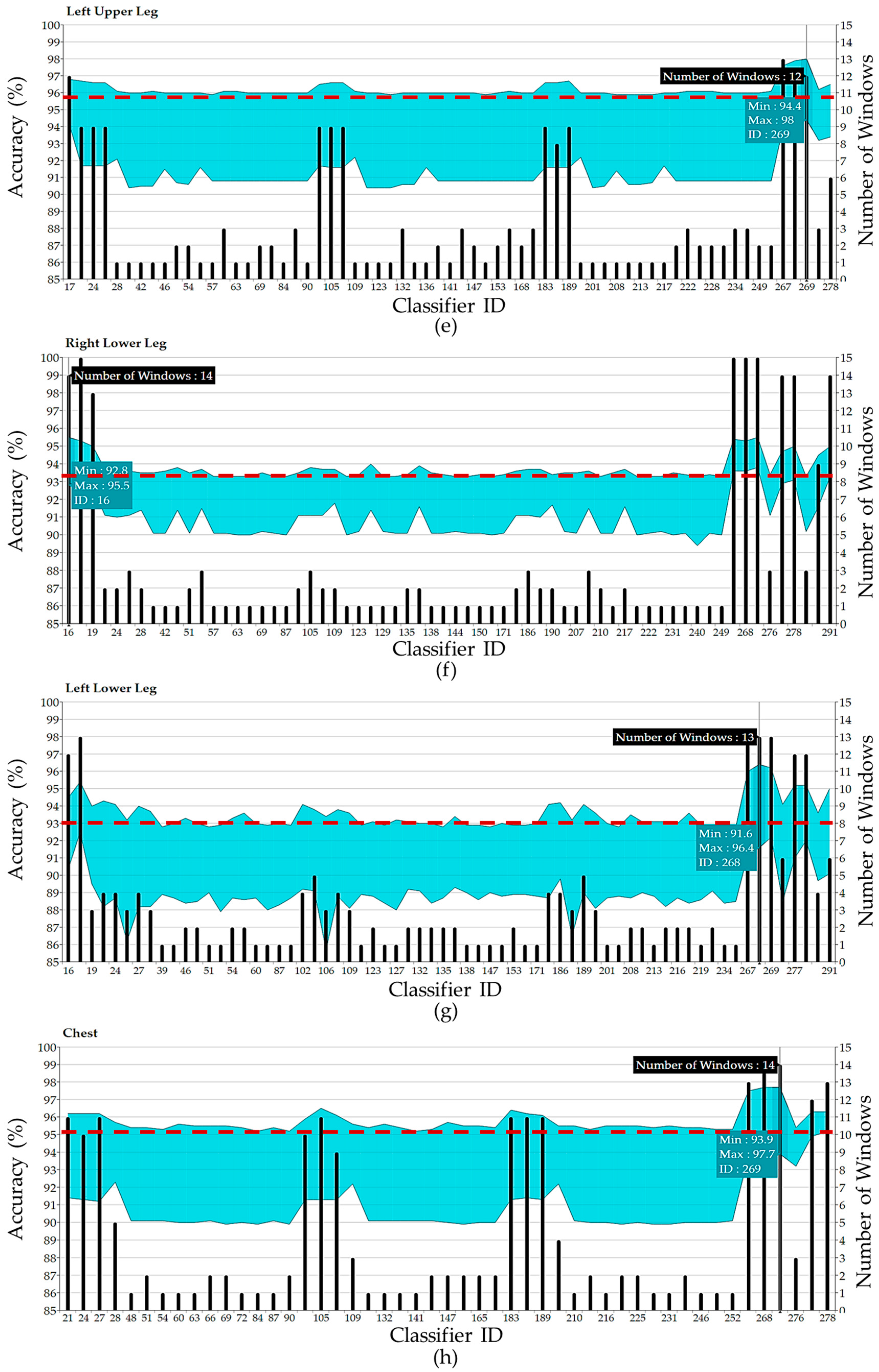
| Waist | Left Upper Leg | ||||||
| 21 | 93.82 | 6.18 | 9.31 | 21 | 96.69 | 3.31 | 3.52 |
| 28 | 94.02 | 5.98 | 9.57 | 24 | 96.62 | 3.38 | 3.39 |
| 108 | 93.75 | 6.25 | 9.24 | 57 | 95.93 | 4.07 | 2.92 |
| 109 | 94.07 | 5.93 | 10.41 | 60 | 96.11 | 3.89 | 3.11 |
| 183 | 93.75 | 6.25 | 8.92 | 222 | 96.15 | 3.85 | 3.16 |
| 189 | 93.72 | 6.28 | 8.80 | 267 | 97.63 | 2.37 | 34.73 |
| 190 | 94.04 | 5.96 | 10.13 | 268 | 97.86 | 2.14 | 102.90 |
| 267 | 95.48 | 4.52 | 45.95 | 269 | 98.03 | 1.97 | 151.83 |
| 268 | 95.51 | 4.49 | 121.58 | Right Lower Leg | |||
| 269 | 95.67 | 4.33 | 196.10 | 16 | 95.52 | 4.48 | 113.05 |
| Right Lower Arm | 24 | 93.82 | 6.18 | 8.03 | |||
| 24 | 93.11 | 6.89 | 7.61 | 28 | 93.45 | 6.55 | 8.02 |
| 102 | 93.29 | 6.71 | 8.01 | 267 | 95.36 | 4.64 | 30.73 |
| 267 | 95.14 | 4.86 | 33.90 | 290 | 94.52 | 5.48 | 8.25 |
| 268 | 95.29 | 4.71 | 87.80 | 291 | 94.97 | 5.03 | 9.14 |
| 269 | 95.30 | 4.70 | 149.78 | Left Lower Leg | |||
| Left Lower Arm | 21 | 94.26 | 5.74 | 7.91 | |||
| 28 | 92.29 | 7.71 | 7.59 | 25 | 93.16 | 6.84 | 7.79 |
| 57 | 91.50 | 8.50 | 7.31 | 267 | 95.99 | 4.01 | 32.36 |
| 63 | 91.61 | 8.39 | 7.35 | 268 | 96.38 | 3.62 | 83.45 |
| 102 | 92.24 | 7.76 | 7.50 | 290 | 93.64 | 6.36 | 7.89 |
| 267 | 94.06 | 5.94 | 32.50 | 291 | 95.02 | 4.98 | 8.85 |
| Right Upper Leg | Chest | ||||||
| 24 | 97.93 | 2.07 | 7.04 | 21 | 96.17 | 3.83 | 6.97 |
| 57 | 97.33 | 2.67 | 6.94 | 84 | 95.25 | 4.75 | 6.58 |
| 63 | 97.43 | 2.57 | 6.94 | 87 | 95.43 | 4.57 | 6.95 |
| 183 | 98.05 | 1.95 | 7.49 | 105 | 96.48 | 3.52 | 7.63 |
| 189 | 97.97 | 2.03 | 7.21 | 168 | 95.39 | 4.61 | 6.91 |
| 267 | 98.85 | 1.15 | 32.12 | 183 | 96.37 | 3.63 | 7.02 |
| 291 | 98.14 | 1.86 | 8.08 | 267 | 97.52 | 2.48 | 29.64 |
| 268 | 97.67 | 2.33 | 76.49 | ||||
| 269 | 97.72 | 2.28 | 125.10 | ||||
© 2017 by the authors. Licensee MDPI, Basel, Switzerland. This article is an open access article distributed under the terms and conditions of the Creative Commons Attribution (CC BY) license ( http://creativecommons.org/licenses/by/4.0/).
Share and Cite
Janidarmian, M.; Roshan Fekr, A.; Radecka, K.; Zilic, Z. A Comprehensive Analysis on Wearable Acceleration Sensors in Human Activity Recognition. Sensors 2017, 17, 529. https://doi.org/10.3390/s17030529
Janidarmian M, Roshan Fekr A, Radecka K, Zilic Z. A Comprehensive Analysis on Wearable Acceleration Sensors in Human Activity Recognition. Sensors. 2017; 17(3):529. https://doi.org/10.3390/s17030529
Chicago/Turabian StyleJanidarmian, Majid, Atena Roshan Fekr, Katarzyna Radecka, and Zeljko Zilic. 2017. "A Comprehensive Analysis on Wearable Acceleration Sensors in Human Activity Recognition" Sensors 17, no. 3: 529. https://doi.org/10.3390/s17030529