A Hybrid Feature Model and Deep-Learning-Based Bearing Fault Diagnosis


Abstract
:1. Introduction
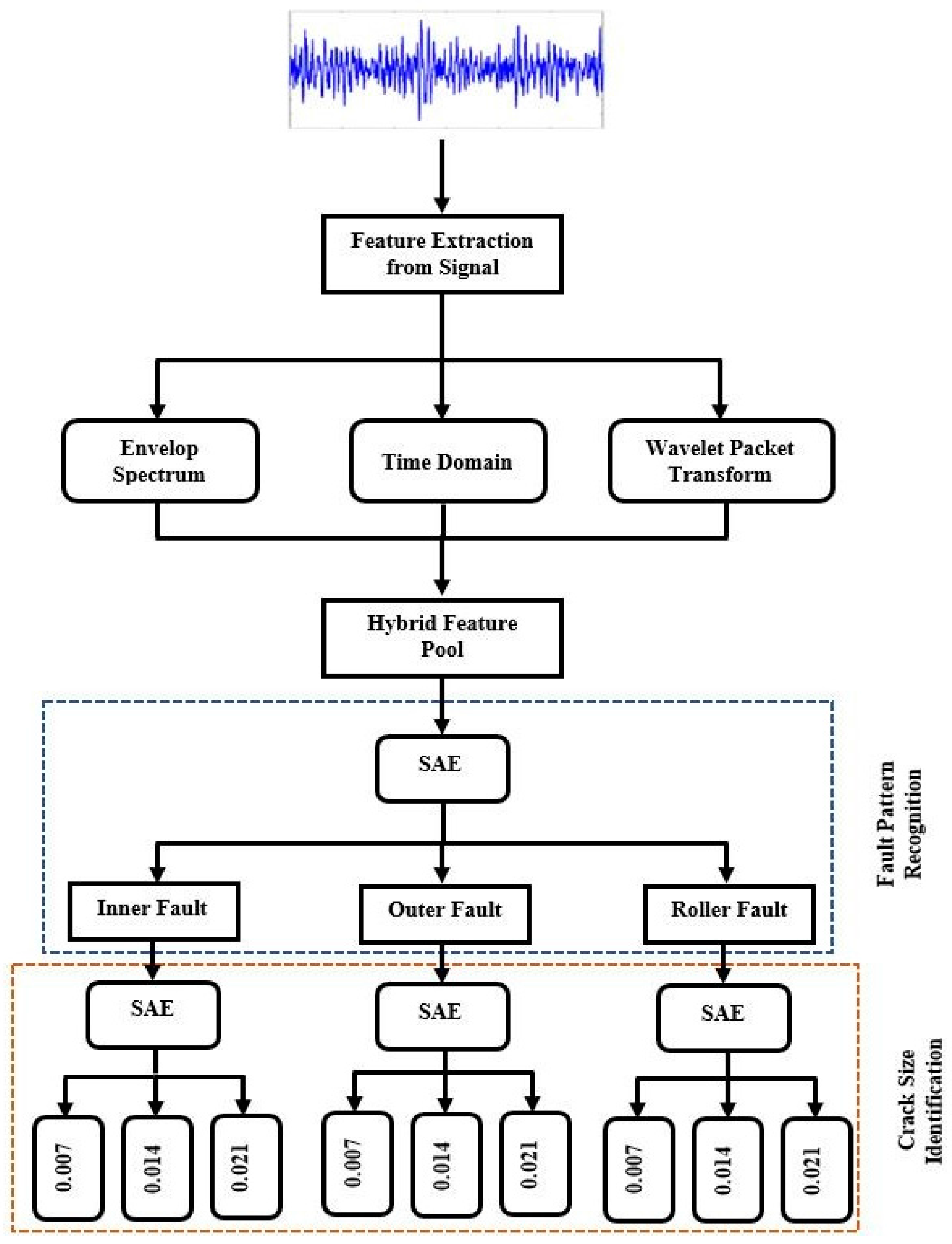
2. Methodology
2.1. Statistical Features
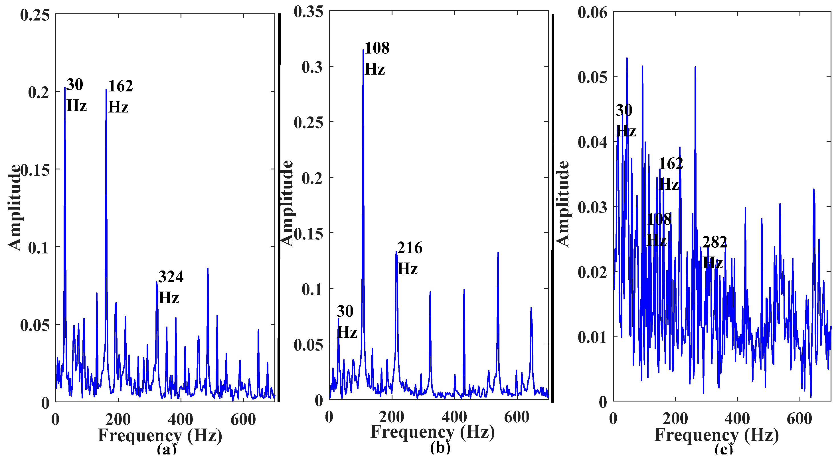
2.2. Envelope Power Spectrum
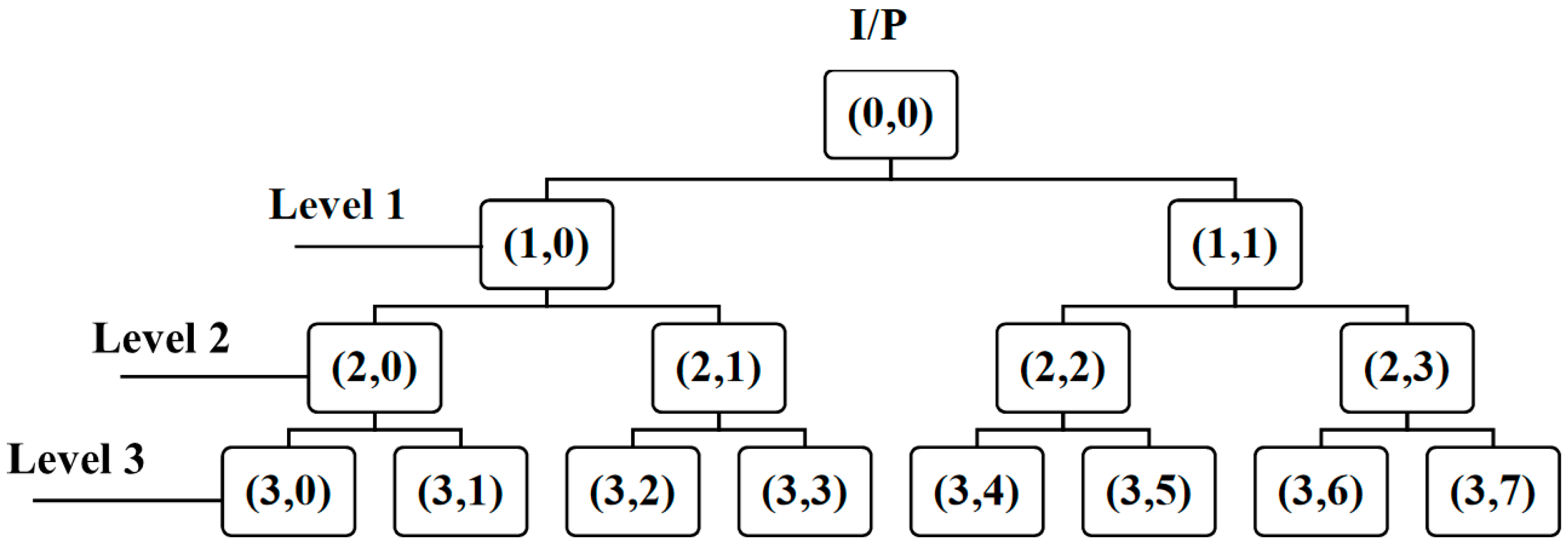
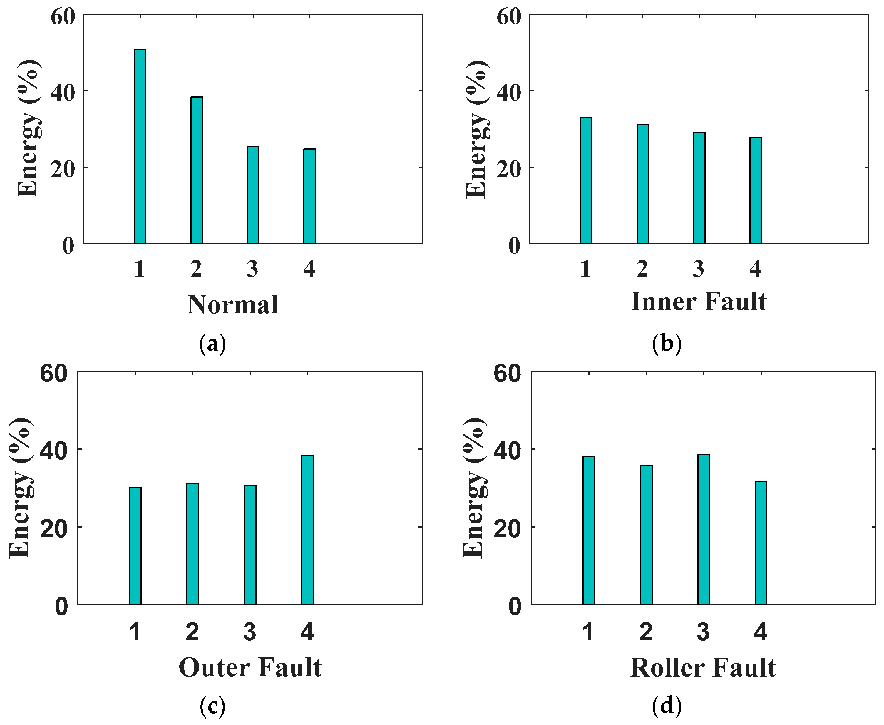
2.3. Wavelet Packet Transform (WPT)
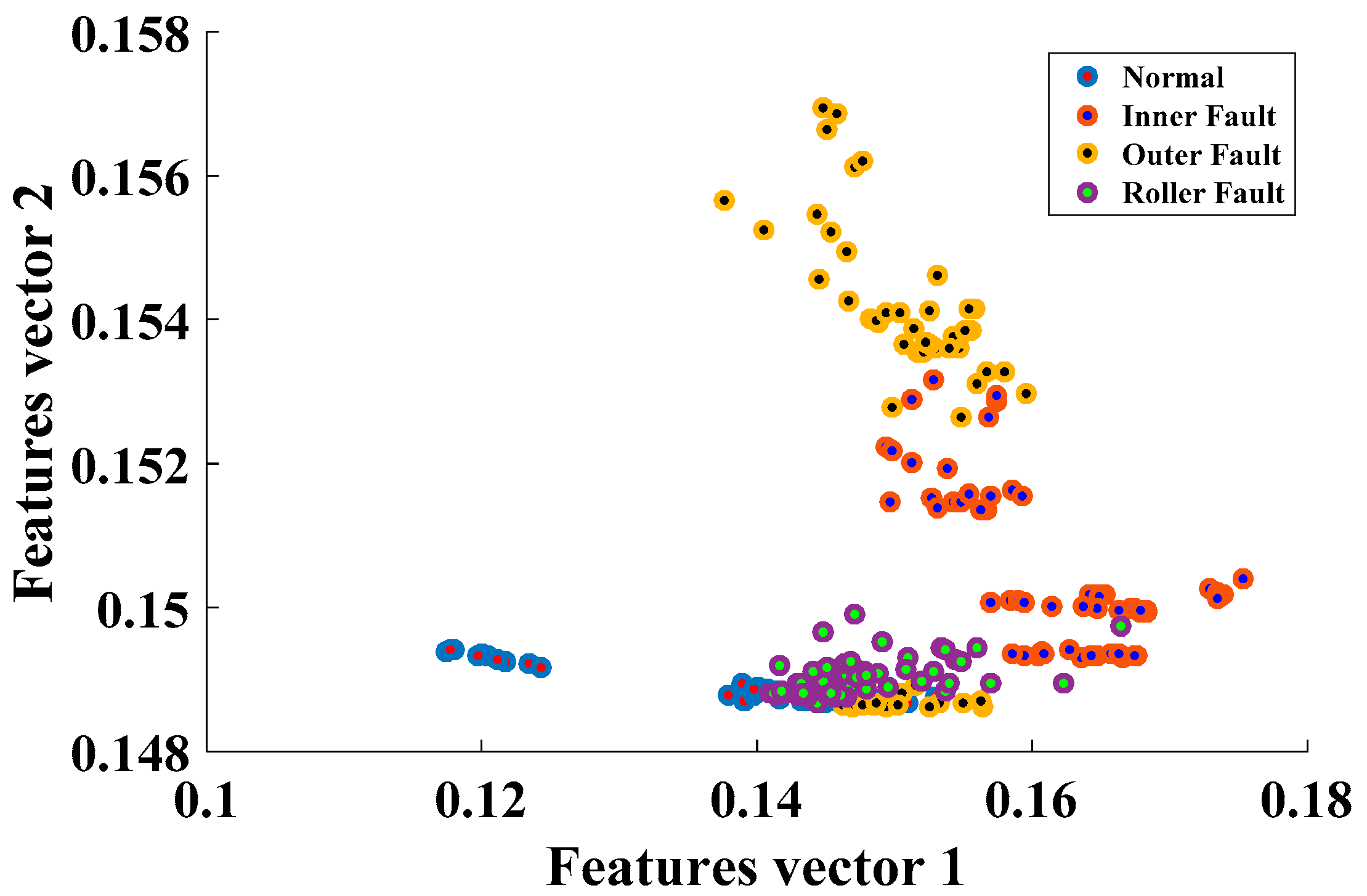
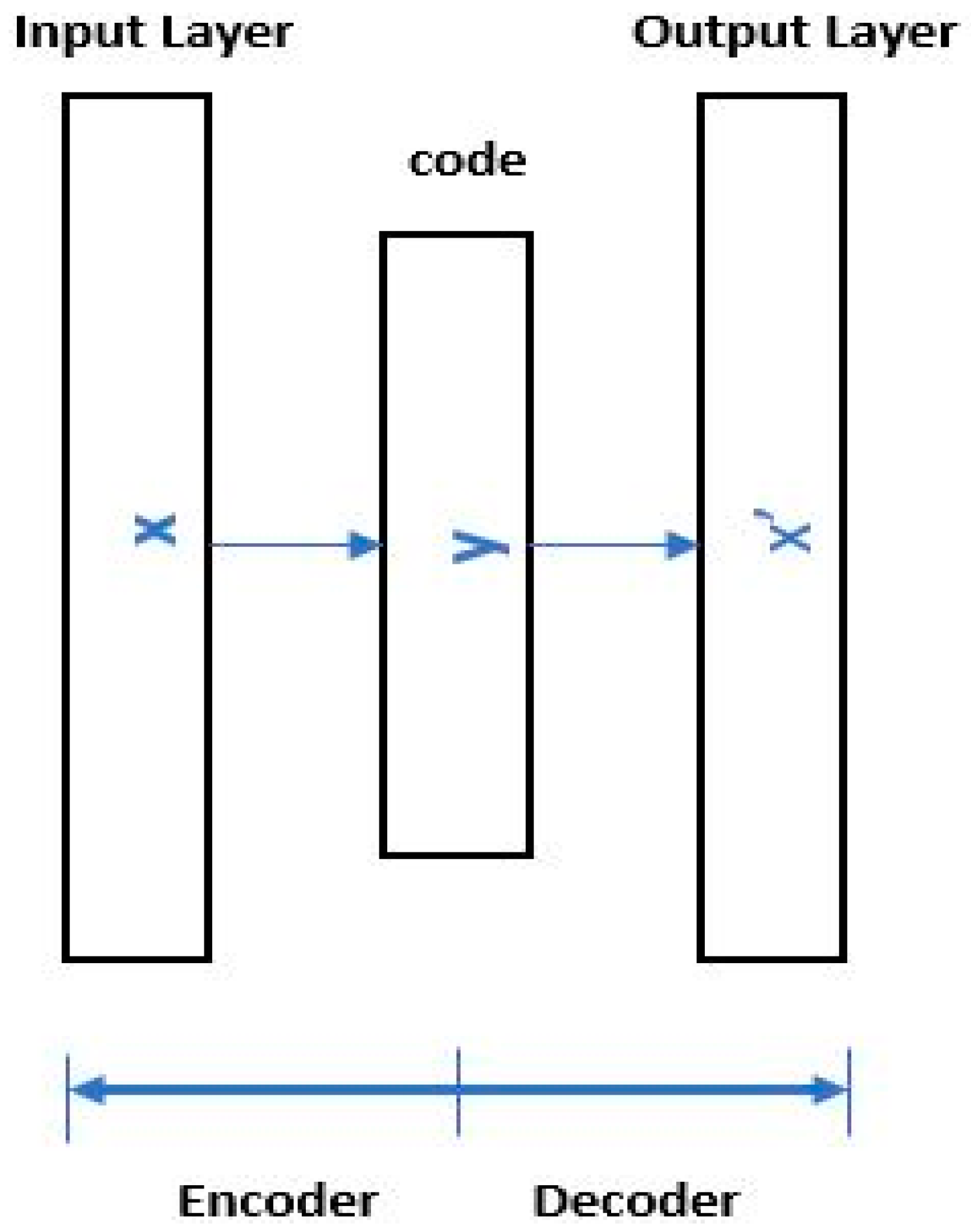
2.4. Sparse Stacked Autoencoders (SSAEs)
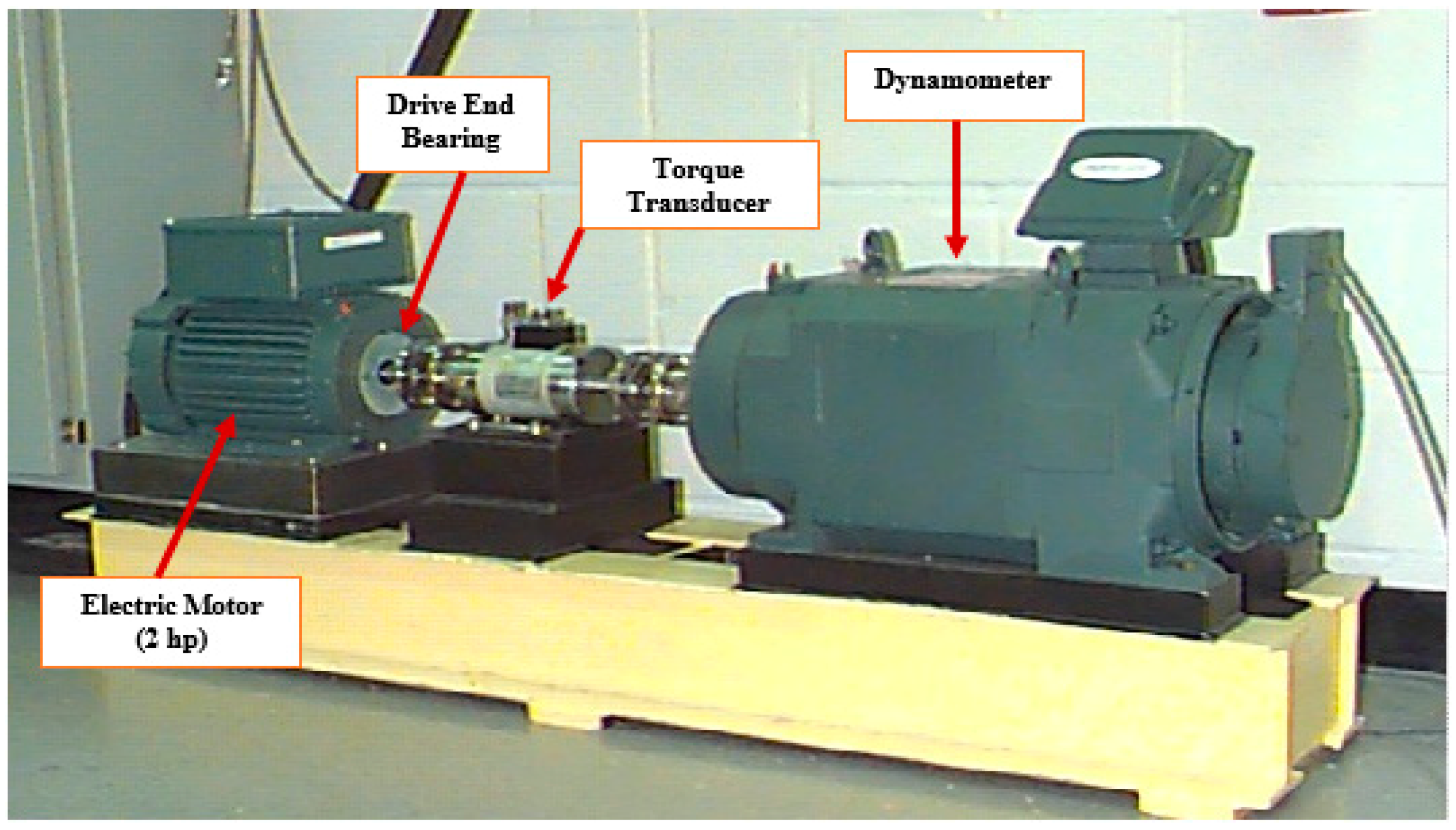
3. Dataset
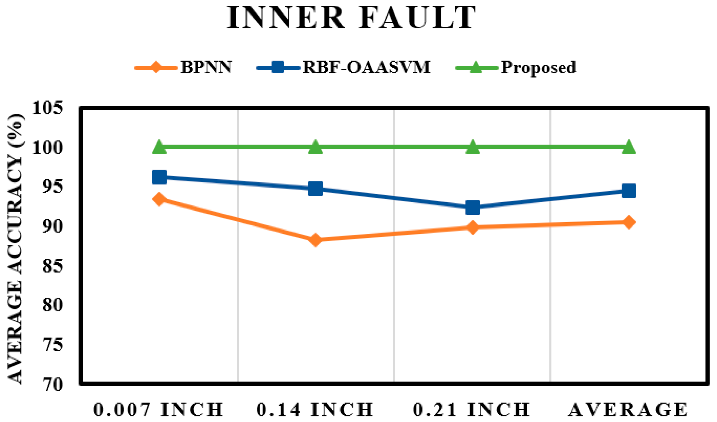
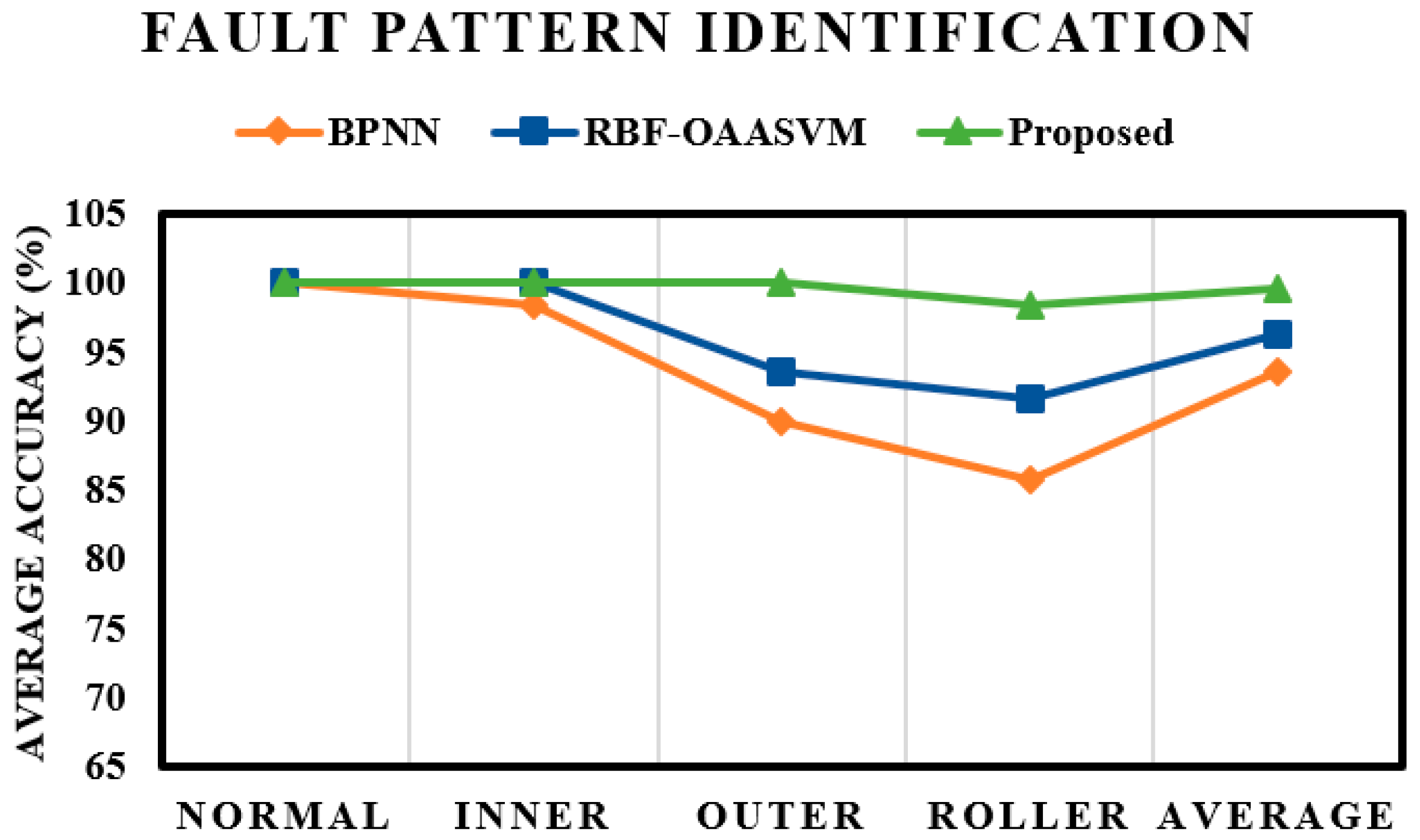
4. Results and Analysis
5. Conclusions
Acknowledgments
Author Contributions
Conflicts of Interest
References
- Toliyat, H.A.; Nandi, S.; Choi, S.; Meshgin-Kelk, H. Electric Machines: Modeling, Condition Monitoring and Fault Diagnosis; CRC Press: Boca Raton, FL, USA, 2012. [Google Scholar]
- Frosini, L.; Harlişca, C.; Szabó, L. Induction machine bearing fault detection by means of statistical processing of the stray flux measurement. IEEE Trans. Ind. Electron. 2015, 62, 1846–1854. [Google Scholar] [CrossRef]
- Islam, M.M.; Kim, J.; Khan, S.A.; Kim, J.-M. Reliable bearing fault diagnosis using Bayesian inference-based multi-class support vector machines. J. Acoust. Soc. Am. 2017, 141, EL89–EL95. [Google Scholar] [CrossRef] [PubMed]
- Khan, S.A.; Kim, J.-M. Automated Bearing Fault Diagnosis Using 2D Analysis of Vibration Acceleration Signals under Variable Speed Conditions. Shock Vib. 2016, 2016. [Google Scholar] [CrossRef]
- Jiang, X.; Wu, L.; Ge, M. A Novel Faults Diagnosis Method for Rolling Element Bearings Based on EWT and Ambiguity Correlation Classifiers. Entropy 2017, 19, 231. [Google Scholar] [CrossRef]
- Li, S.; Liu, G.; Tang, X.; Lu, J.; Hu, J. An Ensemble Deep Convolutional Neural Network Model with Improved DS Evidence Fusion for Bearing Fault Diagnosis. Sensors 2017, 17, 1729. [Google Scholar] [CrossRef] [PubMed]
- Zhang, R.; Peng, Z.; Wu, L.; Yao, B.; Guan, Y. Fault Diagnosis from Raw Sensor Data Using Deep Neural Networks Considering Temporal Coherence. Sensors 2017, 17, 549. [Google Scholar] [CrossRef] [PubMed]
- Youssef, T.; Chadli, M.; Karimi, H.R.; Wang, R. Actuator and sensor faults estimation based on proportional integral observer for TS fuzzy model. J. Frankl. Inst. 2017, 354, 2524–2542. [Google Scholar] [CrossRef]
- Li, L.; Chadli, M.; Ding, S.X.; Qiu, J.; Yang, Y. Diagnostic Observer Design for T-S Fuzzy Systems: Application to Real-Time Weighted Fault Detection Approach. IEEE Trans. Fuzzy Syst. 2017, PP, 1. [Google Scholar] [CrossRef]
- Chibani, A.; Chadli, M.; Shi, P.; Braiek, N.B. Fuzzy Fault Detection Filter Design for T–S Fuzzy Systems in the Finite-Frequency Domain. IEEE Trans. Fuzzy Syst. 2017, 25, 1051–1061. [Google Scholar] [CrossRef]
- Peng, H.; Wang, J.; Ming, J.; Shi, P.; Perez-Jimenez, M.J.; Yu, W.; Tao, C. Fault Diagnosis of Power Systems Using Intuitionistic Fuzzy Spiking Neural P Systems. IEEE Trans. Smart Grid 2017, PP, 1. [Google Scholar] [CrossRef]
- Jardine, A.K.; Lin, D.; Banjevic, D. A review on machinery diagnostics and prognostics implementing condition-based maintenance. Mech. Syst. Signal Process. 2006, 20, 1483–1510. [Google Scholar] [CrossRef]
- Bediaga, I.; Mendizabal, X.; Arnaiz, A.; Munoa, J. Ball bearing damage detection using traditional signal processing algorithms. IEEE Instrum. Meas. Mag. 2013, 16, 20–25. [Google Scholar] [CrossRef]
- Tra, V.; Kim, J.; Khan, S.A.; Kim, J.-M. Incipient fault diagnosis in bearings under variable speed conditions using multiresolution analysis and a weighted committee machine. J. Acoust. Soc. Am. 2017, 142, EL35–EL41. [Google Scholar] [CrossRef] [PubMed]
- Rauber, T.W.; de Assis Boldt, F.; Varejão, F.M. Heterogeneous feature models and feature selection applied to bearing fault diagnosis. IEEE Trans. Ind. Electron. 2015, 62, 637–646. [Google Scholar] [CrossRef]
- Yin, S.; Ding, S.X.; Zhou, D. Diagnosis and prognosis for complicated industrial systems—Part I. IEEE Trans. Ind. Electron. 2016, 63, 2501–2505. [Google Scholar] [CrossRef]
- Yin, S.; Ding, S.X.; Zhou, D. Diagnosis and prognosis for complicated industrial systems—Part II. IEEE Trans. Ind. Electron. 2016, 63, 3201–3204. [Google Scholar] [CrossRef]
- Chang, T.C.; Wysk, R.; Wang, H. Computer-Aided Manufacturing; Prentice Hall: Upper Saddle River, NJ, USA, 1991; p. 7632. [Google Scholar]
- Qin, X.; Li, Q.; Dong, X.; Lv, S. The Fault Diagnosis of Rolling Bearing Based on Ensemble Empirical Mode Decomposition and Random Forest. Shock Vib. 2017, 2017. [Google Scholar] [CrossRef]
- Zhao, S.; Liang, L.; Xu, G.; Wang, J.; Zhang, W. Quantitative diagnosis of a spall-like fault of a rolling element bearing by empirical mode decomposition and the approximate entropy method. Mech. Syst. Signal Process. 2013, 40, 154–177. [Google Scholar] [CrossRef]
- Huang, W.; Sun, H.; Wang, W. Resonance-Based Sparse Signal Decomposition and its Application in Mechanical Fault Diagnosis: A Review. Sensors 2017, 17, 1279. [Google Scholar] [CrossRef] [PubMed]
- Abboud, D.; Antoni, J.; Sieg-Zieba, S.; Eltabach, M. Envelope analysis of rotating machine vibrations in variable speed conditions: A comprehensive treatment. Mech. Syst. Signal Process. 2017, 84, 200–226. [Google Scholar] [CrossRef]
- Zhou, S.; Tang, B.; Chen, R. Comparison between non-stationary signals fast Fourier transform and wavelet analysis. In Proceedings of the International Asia Symposium on Intelligent Interaction and Affective Computing, Wuhan, China, 8–9 December 2009; pp. 128–129. [Google Scholar]
- Torres, R.; Torres, E. Fractional Fourier Analysis of Random Signals and the Notion of/spl alpha/-Stationarity of the Wigner-Ville Distribution. IEEE Trans. Signal Process. 2013, 61, 1555–1560. [Google Scholar] [CrossRef]
- Burriel-Valencia, J.; Puche-Panadero, R.; Martinez-Roman, J.; Sapena-Bano, A.; Pineda-Sanchez, M. Short-Frequency Fourier Transform for Fault Diagnosis of Induction Machines Working in Transient Regime. IEEE Trans. Instrum. Meas. 2017, 66, 432–440. [Google Scholar] [CrossRef]
- Zhang, X.; Jiang, D.; Han, T.; Wang, N.; Yang, W.; Yang, Y. Rotating Machinery Fault Diagnosis for Imbalanced Data Based on Fast Clustering Algorithm and Support Vector Machine. J. Sens. 2017, 2017. [Google Scholar] [CrossRef]
- Islam, M.M.; Kim, J.-M. Time-frequency envelope analysis-based sub-band selection and probabilistic support vector machines for multi-fault diagnosis of low-speed bearings. J. Ambient Intell. Humaniz. Comput. 2017, 1–16. [Google Scholar] [CrossRef]
- Chen, J.; Li, Z.; Pan, J.; Chen, G.; Zi, Y.; Yuan, J.; Chen, B.; He, Z. Wavelet transform based on inner product in fault diagnosis of rotating machinery: A review. Mech. Syst. Signal Process. 2016, 70, 1–35. [Google Scholar] [CrossRef]
- He, S.; Liu, Y.; Chen, J.; Zi, Y. Wavelet Transform Based on Inner Product for Fault Diagnosis of Rotating Machinery. In Structural Health Monitoring; Springer: Cham, Switzerland, 2017; pp. 65–91. [Google Scholar]
- Huang, J.; Chen, G.; Shu, L.; Wang, S.; Zhang, Y. An experimental study of clogging fault diagnosis in heat exchangers based on vibration signals. IEEE Access 2016, 4, 1800–1809. [Google Scholar] [CrossRef]
- Kang, M.; Islam, M.R.; Kim, J.; Kim, J.-M.; Pecht, M. A hybrid feature selection scheme for reducing diagnostic performance deterioration caused by outliers in data-driven diagnostics. IEEE Trans. Ind. Electron. 2016, 63, 3299–3310. [Google Scholar] [CrossRef]
- Tavner, P. Review of condition monitoring of rotating electrical machines. IET Electr. Power Appl. 2008, 2, 215–247. [Google Scholar] [CrossRef]
- Wang, Y.; Xiang, J.; Markert, R.; Liang, M. Spectral kurtosis for fault detection, diagnosis and prognostics of rotating machines: A review with applications. Mech. Syst. Signal Process. 2016, 66, 679–698. [Google Scholar] [CrossRef]
- Dong, S.; Chen, L.; Tang, B.; Xu, X.; Gao, Z.; Liu, J. Rotating machine fault diagnosis based on optimal morphological filter and local tangent space alignment. Shock Vib. 2015, 2015. [Google Scholar] [CrossRef]
- Verstraete, D.; Ferrada, A.; Droguett, E.L.; Meruane, V.; Modarres, M. Deep Learning Enabled Fault Diagnosis Using Time-Frequency Image Analysis of Rolling Element Bearings. Shock Vib. 2017, 2017. [Google Scholar] [CrossRef]
- Yang, D.; Mu, H.; Xu, Z.; Wang, Z.; Yi, C.; Liu, C. Based on Soft Competition ART Neural Network Ensemble and Its Application to the Fault Diagnosis of Bearing. Math. Probl. Eng. 2017, 2017. [Google Scholar] [CrossRef]
- Huo, Z.; Zhang, Y.; Francq, P.; Shu, L.; Huang, J. Incipient fault diagnosis of roller bearing using optimized wavelet transform based multi-speed vibration signatures. IEEE Access 2017, 5, 19442–19456. [Google Scholar] [CrossRef]
- Tahir, M.M.; Khan, A.Q.; Iqbal, N.; Hussain, A.; Badshah, S. Enhancing Fault Classification Accuracy of Ball Bearing Using Central Tendency Based Time Domain Features. IEEE Access 2016, 5, 72–83. [Google Scholar] [CrossRef]
- Yao, B.; Zhen, P.; Wu, L.; Guan, Y. Rolling Element Bearing Fault Diagnosis Using Improved Manifold Learning. IEEE Access 2017, 5, 6027–6035. [Google Scholar] [CrossRef]
- Kang, M.; Kim, J.; Wills, L.M.; Kim, J.-M. Time-varying and multiresolution envelope analysis and discriminative feature analysis for bearing fault diagnosis. IEEE Trans. Ind. Electron. 2015, 62, 7749–7761. [Google Scholar] [CrossRef]
- Xia, Z.; Xia, S.; Wan, L.; Cai, S. Spectral regression based fault feature extraction for bearing accelerometer sensor signals. Sensors 2012, 12, 13694–13719. [Google Scholar] [CrossRef] [PubMed]
- He, D.; Li, R.; Zhu, J. Plastic bearing fault diagnosis based on a two-step data mining approach. IEEE Trans. Ind. Electron. 2013, 60, 3429–3440. [Google Scholar] [CrossRef]
- Dubey, R.; Agrawal, D. Bearing fault classification using ANN-based Hilbert footprint analysis. IET Sci. Meas. Technol. 2015, 9, 1016–1022. [Google Scholar] [CrossRef]
- Nikolaou, N.G.; Antoniadis, I.A. Application of Wavelet Packets in Bearing Fault Diagnosis. In Proceedings of the 5th WSES International Conference on Circuits, Systems, Communications and Computers (CSCC 2001), Rethymno, Greece, 8–15 July 2001; pp. 12–19. [Google Scholar]
- Goodfellow, I.; Bengio, Y.; Courville, A. Deep Learning; MIT Press: Cambridge, MA, USA, 2016. [Google Scholar]
- Case Western Reserve University. B.D.C. Seeded Fault Test Data. Available online: http://csegroups.case.edu/bearingdatacenter/home/ (accessed on 21 January 2017).
- Amar, M.; Gondal, I.; Wilson, C. Vibration spectrum imaging: A novel bearing fault classification approach. IEEE Trans. Ind. Electron. 2015, 62, 494–502. [Google Scholar] [CrossRef]


| Features | Equations | Features | Equations | Features | Equations |
|---|---|---|---|---|---|
| Mean value (MV) | Standard deviation (SD) | Root mean square (RMS) | |||
| Peak-to-peak value (PPV) | Skewness value (SV) | Margin factor (MF) | |||
| Crest factor (CF) | Impulse factor (IF) | Square root of the magnitude (SRM) | |||
| Kurtosis value (KV) | Kurtosis factor (KF) |
| Feature | Equation |
|---|---|
| RMS frequency | |
| Frequency center | |
| Standard deviation | |
| Root variance frequency | |
| Spectral kurtosis |
| Fault Type | Fault Location | Fault Size (Inches) | Training Samples | Test Samples | Sample Length | Accelerometer Position | Shaft Load (hp) |
|---|---|---|---|---|---|---|---|
| Normal | None | 0 | 40 | 30 | 12,000 | Drive End Bearings | 0, 1, 2, 3 |
| Inner raceway | IR | 0.007 | 30 | 30 | |||
| IR | 0.014 | 30 | 30 | ||||
| IR | 0.021 | 30 | 30 | ||||
| Outer raceway | OR | 0.007 | 30 | 30 | |||
| OR | 0.014 | 30 | 30 | ||||
| OR | 0.021 | 30 | 30 | ||||
| Roller | RE | 0.007 | 30 | 30 | |||
| RE | 0.014 | 30 | 30 | ||||
| RE | 0.021 | 30 | 30 |
| Method | Layer 1 Average Accuracy (%) | Layer 2 Average Accuracy (%) | Total (%) | ||
|---|---|---|---|---|---|
| 0.007 Inches | 0.014 Inches | 0.021 Inches | |||
| VSI [47] | 60.15 | 55 | 55 | 84.6 | 63.68 |
| Proposed | 99.75 | 100 | 100 | 96.66 | 99.10 |
© 2017 by the authors. Licensee MDPI, Basel, Switzerland. This article is an open access article distributed under the terms and conditions of the Creative Commons Attribution (CC BY) license (http://creativecommons.org/licenses/by/4.0/).
Share and Cite
Sohaib, M.; Kim, C.-H.; Kim, J.-M. A Hybrid Feature Model and Deep-Learning-Based Bearing Fault Diagnosis. Sensors 2017, 17, 2876. https://doi.org/10.3390/s17122876
Sohaib M, Kim C-H, Kim J-M. A Hybrid Feature Model and Deep-Learning-Based Bearing Fault Diagnosis. Sensors. 2017; 17(12):2876. https://doi.org/10.3390/s17122876
Chicago/Turabian StyleSohaib, Muhammad, Cheol-Hong Kim, and Jong-Myon Kim. 2017. "A Hybrid Feature Model and Deep-Learning-Based Bearing Fault Diagnosis" Sensors 17, no. 12: 2876. https://doi.org/10.3390/s17122876