Robust Radar Emitter Recognition Based on the Three-Dimensional Distribution Feature and Transfer Learning

Abstract

Due to the increasing complexity of electromagnetic signals, there exists a significant challenge for radar emitter signal recognition. To address this challenge, multi-component radar emitter recognition under a complicated noise environment is studied in this paper. A novel radar emitter recognition approach based on the three-dimensional distribution feature and transfer learning is proposed. The cubic feature for the time-frequency-energy distribution is proposed to describe the intra-pulse modulation information of radar emitters. Furthermore, the feature is reconstructed by using transfer learning in order to obtain the robust feature against signal noise rate (SNR) variation. Last, but not the least, the relevance vector machine is used to classify radar emitter signals. Simulations demonstrate that the approach proposed in this paper has better performances in accuracy and robustness than existing approaches.

1. Introduction

Radar emitter recognition (RER) based on a collection of received radar signals is a specific type of identification termed specific emitter identification (SEI), which is used to distinguish different copies of the same type of radar emitter [1,2,3,4]. RER is a topic of wide interest in both military and civil applications [5,6]. In military applications, radar emitter recognition is a critical issue in radar reconnaissance systems [7]. Specifically, radar emitter recognition provides an important means of detecting hostile radar targets. In civilian applications, radar emitter recognition technology is used to suppress criminal activities by identifying navigation radars deployed on cars and ships [5]. However, the growing complexity of electromagnetic signals encountered in modern environments is a challenge for radar emitter signal recognition [7]. Traditional approaches are becoming inefficient against this emerging issue, especially when several radar emitter signals are captured [8,9]. Therefore, multi-component radar emitter recognition under a complicated noise environment is a challenge.

Many research works have been done, e.g., stochastic context-free grammar analysis [7,10], symbolic time series analysis [11,12,13] and time-frequency analysis [14,15,16,17,18,19]. Thereinto, time-frequency representation (TFR) has been frequently used for the analysis, the detection and the classification of nonstationary signals [20,21,22,23]. In [24], Swiercz proposed automatic classification of linear frequency modulation (LFM)signals for radar emitter recognition using wavelet decomposition and learning vector quantization (LVQ) classifier. In [25], a radar emitter recognition approach is proposed by using a classifier combining a minimum Mahalanobis distance classifier and SVM, which can recognize the numbers of intra-pulse modulation radar emitter signals. In [26], a hybrid radar emitter recognition is proposed. In [27], a robust radar emitter recognition based on fuzzy theory is proposed, which can recognize radar emitters robustly to some extent. However, these approaches have certain limitations for recognizing radar emitters in a complicated noise environment, which necessitates further investigation of robust radar emitter recognition.

Against this background, this research aims at proposing a robust scheme for multi-component radar emitter recognition under a complicated noise environment. The remainder of this paper is organized as follows. Section 2 gives the novel radar emitter recognition approach followed by the simulation and numerical analysis in Section 3. This paper is concluded in Section 4.

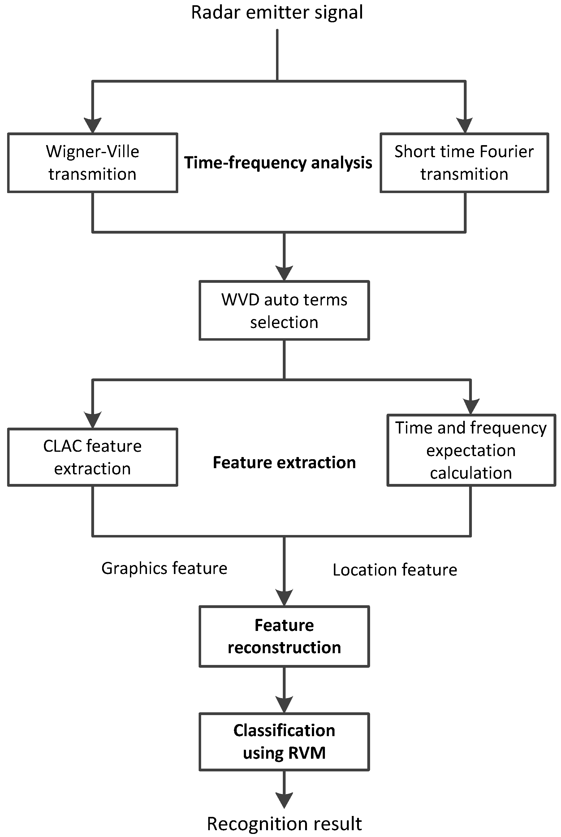
2. Radar Emitter Recognition System

2.1. System Model

The multi-component radar emitter recognition under complicated noise environment is studied in this paper. A radar emitter recognition approach based on the three-dimensional distribution feature and transfer learning are proposed. The process of radar emitter recognition is shown in Figure 1.

Three functional modules are included in this research:

• time-frequency analysis,
• feature extraction,
• classification.

The time-frequency analysis is a preprocess of feature extraction and has been well known as a well-developed technique [28]. In this paper, the Wigner–Ville distribution (WVD) is used to represent the characteristics of radar emitters. However, the WVD cross terms are interferences of feature extraction. Therefore, the WVD cross terms are suppressed by using a superimposition of multiple spectrograms method [29]. The auto WVDs of radar signals are detected.

In the feature extraction block, a hybrid feature is extracted, which consists of a graphics feature and a location feature. Since redundancy features are contained in the graphics features, these features would be reconstructed. Feature reconstruction is based on transfer learning.

After sorting and feature extraction, radar emitter signals are described by vectors. These describing vectors are used for classification by using RVM.

2.2. Time-Frequency Analysis of Radar Emitter Signals

WVD is a famous time-frequency distribution method, which is widely used in signal processing for its good information-preserving property. The WVD of a given signal $x\left(t\right)$ is defined by:

$$W_x\left(t,f\right)={\int }_{-\infty }^{+\infty }{R}_x\left(t,\tau \right)exp\left(-2\pi jf\tau \right)d\tau$$

(1)

$$R_x(t,\tau )=x\left(t+\frac{\tau }{2}\right)x^{*}\left(t-\frac{\tau }{2}\right)$$

(2)

where τ denotes the dummy variable; * and $W_x(t,f)$ denote the complex conjugate and the energy distribution of $x\left(t\right)$ in frequency f at time t, respectively.

However, a criticism against WVD in application is the cross term, which is caused by the presence of several signal components. In order to suppress the cross terms caused by multi-component signals and noise, a suppression method by using the superimposition of multiple spectrograms is adopted. The spectrogram of the input signal can be obtained by the square of the short time Fourier transformation. Let $f\left(t\right)$ be the input signal sampling value, namely $f\left(t\right)=x(n\Delta t)$, where $0\le n<N$. Therefore, in the case of the discrete signals, the short time Fourier transformation is given by:

$$S_{f,L_t,\beta }\left(n,k\right)={\sum }_{m=0}^{N-1}f\left(m\right){g^{*}}_{L_t,\beta }(m-n)exp\left(-\frac{2\pi mk}{N}\right)$$

(3)

$$g_{L_{t,\beta }}\left(n\right)=\frac{1}{\sqrt[4]{\pi L_t^2}}exp\left\{-\frac{n^2}{2L_t^2}+j\frac{\beta }{2}{n}^2\right\}$$

(4)

where $g_{L_i,\beta }\left(n\right)$ is a discrete window function, $L_t={\sigma }_t/\phantom{{\sigma }_t\Delta t}\Delta t$, $\beta =\eta \Delta t^2$.

The discrete signal spectrogram is given by:

$$D_f\left(n,k\right)=\frac{1}{I+1}{\sum }_{i=0}^I{\left|S_{f,L_i,\beta }\left(n,k\right)\right|}^2$$

(5)

Auto term regions of the spectrogram can be determined by judging $D_f\left(n,k\right)$ using a threshold, i.e.,

$$\Omega =\left\{\left(n,k\right):D_f\left(n,k\right)\ge \eta \right\}$$

(6)

where η is the threshold, which is given by:

$$\eta =max\left\{\mu :{\sum }_{D_f\left(n,k\right)\ge \mu }{D}_f\left(n,k\right)\ge \gamma {\sum }_{n=0}^{N-1}{\left|f\left(n\right)\right|}^2\right\}$$

(7)

where γ is a factor, which means the ratio of the energy of the auto-term region against the whole WVD. It is proven by experiments that γ is between 0.7 and 0.98 [29,30], and we shall use 0.8 in this paper.

The auto-terms of WVD are obtained by determining regions, which is given by:

$$\begin{array}{c}\hfill W_{auto}\left(n,k\right)=S_{\Omega }\left(n,k\right)W_f\left(n,k\right)\end{array}$$

(8)

$$\begin{array}{c}\hfill S_{\Omega }\left(n,k\right)=\left\{\begin{array}{c}1,\begin{array}{cc}& \left(n,k\right)\in \Omega \end{array}\\ 0,\begin{array}{cc}& \left(n,k\right)\notin \Omega \end{array}\end{array}\right\}\end{array}$$

(9)

Then, the auto-terms of WVD are obtained. The excellent mathematical properties of WVD are inherited. The expression of the interaction among the time, frequency and energy of a radar emitter is given in the form of WVD auto-terms. The auto-terms of WVD are normalized in each dimension and then used as the input of feature extraction. The approach to obtain the WVD auto-terms is stated with more details in [30].

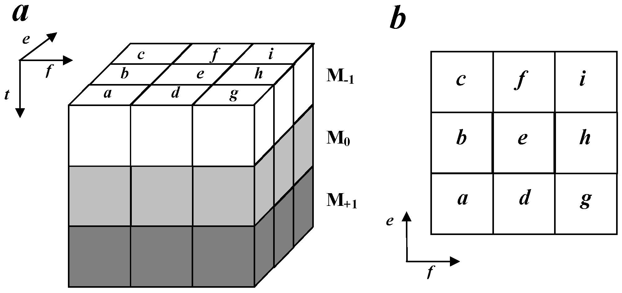
2.3. Feature Extraction

The information of the distribution in dimensions of time, frequency and energy is an effective characteristic to distinguish different radar emitter signals. To extract the effective information in radar emitter signal pulses, a three-dimensional distribution feature is proposed, which consists of two parts, namely, the graphics feature and the location feature. This feature is used to extract information on WVDs of radar emitter targets.

The graphics feature is based on the cubic local auto-correlation (CLAC) function. The cubic local auto-correlation function is used for feature extraction and was proposed by Otsu in 2009 [31], which is an efficient way to describe three-dimensional distributions. The WVD-based CLAC feature is proposed and adopted as a graphics feature in this paper. A brief introduction of WVD-based CLAC feature is as follows.

Let $g\left(\mathbf{r}\right)$ be three-way (cubic) data defined on the region $D:T\times F\times E$ with $\mathbf{r}={(t,f,e)}^{\mathrm{T}}$, where F and E denote the frequency and energy of the radar emitter signal, respectively, and T is the time length of the time window. Then, the N-th order auto-correlation function is defined by:

$$\begin{array}{cc}& R_N({\mathbf{a}}_1,···,{\mathbf{a}}_N)={\int }_{D_S}g\left(\mathbf{r}\right)g(\mathbf{r}+{\mathbf{a}}_1)···g(\mathbf{r}+{\mathbf{a}}_N)d\mathbf{r}\hfill \\ & D_S=\left\{\mathbf{r}\right|\mathbf{r}+{\mathbf{a}}_i\in D\forall i\}\hfill \end{array}$$

(10)

where ${\mathbf{a}}_i(i=1,···,N)$ denote displacement vectors from the reference point $\mathbf{r}$. We limit $N\le 2$ and ${\mathbf{a}}_i$ to a local region of a cube centering on $\mathbf{r}$. A CLAC feature (vector) is made up of $R_N({\mathbf{a}}_1,···,{\mathbf{a}}_N)$ with various ${\mathbf{a}}_1,···,{\mathbf{a}}_N$ in the local region. The computation of CLAC features is described as follows.

Firstly, Equation (10) is translated to a corresponding discrete version as Equation (11) shows,

$$R_N({\mathbf{a}}_1,...,{\mathbf{a}}_N)=\sum _{t,f,e\in D_S}g(t,f,e)g(t+a_{1t},f+a_{1f},e+a_{1e})···g(t+a_{Nt},f+a_{Nf},e+a_{Ne})$$

(11)

where $a_{ie},a_{if},a_{it}\in \left\{\pm \Delta r,0\right\}$ and $N\in \{0,1,2\}$, namely the same shifting distances are exploited in t, f and e dimensions. Then, the N-th-order autocorrelation function of binary images can be regarded as counting the number of points satisfying some logical condition, namely,

$$g\left(r\right)\wedge g\left(r+a_1\right)\wedge ···\wedge g\left(r+a_N\right)=1$$

(12)

Therefore, the N-th-order autocorrelation function can be transformed into counting the patterns characterized by the above logical statement over g. Obviously, the scan by the reference point $(t,f,e)$ can be restricted to the“1” points, viz., $g\left(r\right)=1$, in g. The configuration $(\mathbf{r},\mathbf{r}+{\mathbf{a}}_{\mathbf{1}},···,\mathbf{r}+{\mathbf{a}}_{\mathbf{N}})$ is represented by a local mask pattern.

Let M be the reference space insisting of 27 space units, as shown in Figure 2. In M, there are three layers, namely $M_{-1},M_0,M_{+1}$, and positions in each layer are termed $a,b,c,d,e,f,g,h,i$.

Each space unit in M is given a weight, which is $2^n$ $\left(n\in \left[0,1,···,26\right]\right)$. The convolution between M and the hyperplane of a WVD auto-term in the (t, f, e) space is carried out, which is given by:

$$C\left(t,f,e\right)=\sum _t\sum _f\sum _{e}M\left(t^{\prime },f^{\prime },e^{\prime }\right)W\left(t-t^{\prime },f-f^{\prime },e-e^{\prime }\right)$$

(13)

where $W(t,f,e)$ denotes the discrete WVD auto-term. Then, the number of each mask pattern in WVD is counted by comparing the convolution result matrix and flag values of mask patterns. The numbers of mask patterns are used as features.

Obviously, no more than three points can denote the N-th-order autocorrelation ($N=0,1,2$). There are many possible mask patterns, including duplicated patterns in terms of point configurations, and these mask patterns are reduced. In the case of binary image ($f\left(\mathbf{r}\right)$ = 0 or 1), $f{\left(\mathbf{r}\right)}^k=f\left(\mathbf{r}\right),\forall k>0$. The number of mask patterns is reduced to 251. Since the dimension of CLAC features corresponds to the number of mask patterns, we shall use the 251 dimensions features as the graphics features.

However, due to the shift-invariance of the autocorrelation, in the case that the point configuration of $({\mathbf{r}}^{\left(1\right)},{\mathbf{r}}^{\left(1\right)}+{\mathbf{a}}_1^{\left(1\right)},···,{\mathbf{r}}^{\left(1\right)}+{\mathbf{a}}_N^{\left(1\right)})$ matches that of $({\mathbf{r}}^{\left(2\right)},{\mathbf{r}}^{\left(2\right)}+{\mathbf{a}}_1^{\left(2\right)},···,{\mathbf{r}}^{\left(2\right)}+{\mathbf{a}}_N^{\left(2\right)})$ by shifting, $R_N(a_1^{\left(1\right)},···,a_N^{\left(1\right)})$ will have the same value as $R_N(a_1^{\left(2\right)},···,a_N^{\left(2\right)})$, which may lead to the confusion about the difference among targets with a similar WVD distribution. Therefore, positional information is adopted, so as to address the confusion caused by shifting in time and frequency. We locate the target WVD auto-term by computing the gravity center, which is represented by the time and frequency expectations. The time and frequency expectations of a WVD are given by:

$${\widehat{t}}_{\Omega }\left(t,f\right)=\frac{{\int }_{-\infty }^{+\infty }{t}^{\prime }\Omega \left(t^{\prime }-t,f^{\prime }-f\right)W_x\left(t^{\prime },f^{\prime }\right)d{t}^{\prime }d{f}^{\prime }}{E_{\Omega }\left(t,f\right)}$$

(14)

$${\widehat{f}}_{\Omega }\left(t,f\right)=\frac{{\int }_{-\infty }^{+\infty }{f}^{\prime }\Omega \left(t^{\prime }-t,f^{\prime }-f\right)W_x\left(t^{\prime },f^{\prime }\right)d{t}^{\prime }d{f}^{\prime }}{E_{\Omega }\left(t,f\right)}$$

(15)

where the $E_{\Omega }$ denotes the energy in region Ω.

In this paper, the gravity center position of the WVD auto-term is termed as the location feature.

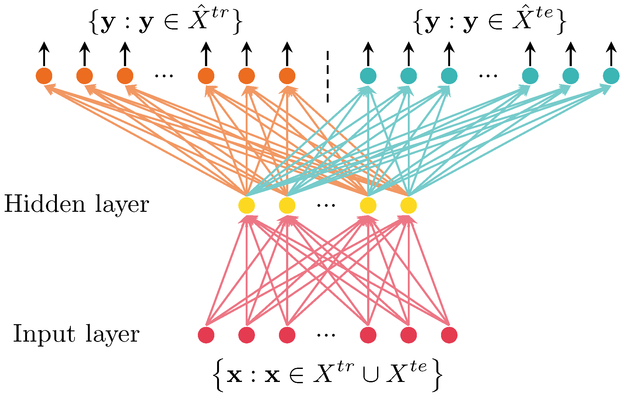
2.4. Feature Learning Based on Transfer Learning

In order to characterize different radar emitter targets, the 3D feature is extracted. However, this feature has a very large number of dimensions, i.e., 251 dimensions, which results in much redundant information for recognition. Therefore, the dimension reduction should be adopted. On the other hand, the variation of the signal noise rate (SNR) is an adverse effect on radar emitter recognition. Hence, a feature reconstruction approach based on transfer learning is adopted in this paper. By feature reconstruction, the robust feature against SNR variation is obtained, and the dimension of the feature is reduced, simultaneously.

Transfer learning is proposed to deal with the problem of how to reuse the knowledge learned previously from other data or features [32,33]. The idea behind transfer learning is to exploit the common knowledge between different learning tasks in order to share statistical strength and transfer knowledge across tasks [33,34,35]. In this paper, the learning task is to transfer common knowledge among recognitions in different noise environments.

The shared-hidden-layer autoencoder (SHLA) is an efficient approach for transfer learning [36]. It is utilized to obtain the compendious feature set with common knowledge from the original feature set. The structure of the SHLA is shown in Figure 3.

As shown, the target values are set to be equal to the input, and the hidden representation $h\left(x\right)$ is:

$$h\left(x\right)=f\left(W_{1}x+b_1\right)$$

(16)

where $f\left(z\right)$ is a non-linear activation function, $f\left(z\right)=1/(1+exp(z\left)\right)$, $W_1$ is a weight matrix and $b_1$ is a bias vector.

The network output maps the hidden representation h back for the reconstruction of $\tilde{x}$:

$$\tilde{x}=f\left(W_{2}h\left(x\right)+b_2\right)$$

(17)

where $W_2$ is a weight matrix and $b_2$ is a bias vector.

In SHLA, same parameters for the mapping are shared between the input layer and the hidden layer. However, independent parameters are used in the reconstruction process. Let $X_{tr}$ be the training set and $X_{te}$ be the test set. Two objective functions are given by:

$$j_{tr}\left({\theta }_{tr}\right)=\sum _{x\in {\chi }^{tr}}{∥x-\tilde{x}∥}^2$$

(18)

$$j_{te}\left({\theta }_{te}\right)=\sum _{x\in {\chi }^{te}}{∥x-\tilde{x}∥}^2$$

(19)

where the parameters ${\theta }_{tr}=\{W_1,W_2^{tr},b_1,b_2^{tr}\}$ and ${\theta }_{te}=\{W_1,W_2^{te},b_1,b_2^{te}\}$ share the same parameters $\{W_1,b_1\}$.

Besides, the overall objective function is obtained by joining the two parts, given by:

$$j_{SA}\left({\theta }_{SA}\right)=j_{tr}\left({\theta }_{tr}\right)+\gamma j_{te}\left({\theta }_{te}\right)$$

(20)

where ${\theta }_{SA}=\left\{W_1,W_2^{tr},W_2^{te},b_1,b_2^{tr},b_2^{te}\right\}$, which will be optimized during training; γ is the hyper-parameter to control the strength of regularization.

In training, the back-propagation algorithm is adopted. The shared hidden layer makes the distribution induced by the training set similar to the distribution induced by the target set. Autoencoders find the useful features hidden in data automatically. This approach is wildly used in building a deep feature hierarchy, under the modelings of unsupervised, supervised and semi-supervised [37,38]. In this research, the reconstructed feature can be obtained from the hidden layer in SHLA for radar emitter robust recognition against SNR variation.

2.5. Classification Using RVM

The relevance vector machine (RVM), which is a sparse Bayesian modeling approach, is proposed by in [39,40]. RVM provides an approach for sparse classification. A small number of fixed basis functions are selected from a large potential candidate dictionary and weighted linearly. Therefore, a significant advantage of RVM is free from the satisfying Mercer’s condition of kernel functions.

For binary classification, the likelihood function is given by:

$$\mathrm{P}\left(\mathbf{t}|\mathit{\omega }\right)=\prod _{n-1}^N\sigma {\left\{y\left(x_n,\mathit{\omega }\right)\right\}}^{t_n}{\left[1-\sigma \left\{y\left(x_n,\mathit{\omega }\right)\right\}\right]}^{1-t_n}$$

(21)

where $t_n\in (0,1)$ denotes the target value; ω is a Gauss conditional probability, which has zero expectation and variance ${\alpha }_i^{-1}$.

The maximum posterior probability estimation can be found by seeking the mode point of the Gaussian function, i.e., ${\mu }_{MP}$.

Due to:

$$\mathrm{P}\left(\mathit{\omega }|\mathbf{t},\mathit{\alpha }\right)=\frac{\mathrm{P}\left(\mathbf{t}|\mathit{\omega }\right)\mathrm{P}\left(\mathit{\omega }|\mathit{\alpha }\right)}{\mathrm{P}\left(\mathbf{t}|\mathit{\alpha }\right)}$$

(22)

the posterior probability according to ω can be maximized by maximizing:

$$\begin{array}{c}log\left\{\mathrm{P}\left(\mathit{\omega }|\mathbf{t},\alpha \right)\right\}=log\left\{\mathrm{P}\left(\mathbf{t}|\mathit{\omega }\right)\right\}+log\left\{\mathrm{P}\left(\mathit{\omega }|\alpha \right)\right\}-log\left\{\mathrm{P}\left(\mathbf{t}|\alpha \right)\right\}\hfill \\ ={\displaystyle \sum _{n=1}^N}\left[t_{n}log{y}_n+\left(1-t_n\right)log\left(-y_n\right)\right]-\frac{1}{2}{\mathit{\omega }}^{\mathrm{T}}\mathit{A}\mathit{\omega }+c\hfill \end{array}$$

(23)

where $y_n=\sigma \left\{y\left(x_n,\mathit{\omega }\right)\right\}$ and c is a constant.

The marginal likelihood function is given by:

$$\mathrm{P}\left(\mathit{\omega }|\mathbf{t},\alpha \right)=\int \mathrm{P}\left(\mathbf{t}|\mathit{\omega }\right)\mathrm{P}\left(\mathit{\omega }|\alpha \right)\mathrm{d}\mathit{\omega }\simeq \mathrm{P}\left(t|{\mathit{\omega }}_{MP}\right)\mathrm{P}\left({\mathit{\omega }}_{MP}|\alpha \right){\left(2\pi \right)}^{M/\phantom{M2}2}{\left|\Sigma \right|}^{1/\phantom{12}2}$$

(24)

Suppose $\widehat{\mathbf{t}}$ is the approximation of the Gaussian posterior distribution, with ${\mu }_{MP}=\Sigma {\Phi }^T\mathbf{B}\widehat{\mathbf{t}}$ and $\Sigma ={\left({\Phi }^T\mathbf{B}\Phi +\mathbf{A}\right)}^{-1}$. Sparse Bayesian learning can then be formulated as a type-II maximum likelihood procedure. The logarithm of approximate marginal likelihood function is given by:

$$log\mathrm{p}\left(\mathbf{t}|\alpha \right)=-\frac{1}{2}\left\{Nlog\left(2\pi \right)+log\left|\mathbf{C}\right|+{\widehat{\mathbf{t}}}^{\mathbf{T}}{\mathbf{C}}^{-1}\widehat{\mathbf{t}}\right\}$$

(25)

where $\mathbf{C}=\mathbf{B}+\Phi {\mathbf{A}}^{-1}{\Phi }^T$.

Fast marginal likelihood maximization for sparse Bayesian models is exploited in this paper. More details of the fast approach can be found in [40].

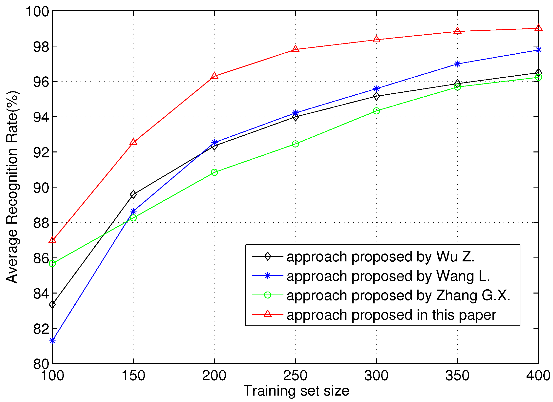
3. Results and Discussion

The validity and robustness of the proposed approach will be evaluated by simulations. We investigate the performance of the proposed framework on an emulation dataset, which consists of six types of radar emitter targets generated emulationally based on the information of radars in the National Missile Defense (NMD) system [41]. In this dataset, mono-pulse radar and pulse compression radar are involved. The intra-pulse modulation types consist of linear frequency modulation (LFM), binary phase shift keying (BPSK) and quadri-phase shift keying (QPSK). The parameters of these radar emitter targets are given in detail by

Table 1. Information of radar emitter targets. PW, pulse width; FTR, frequency-time rate; CS, coding scheme; LFM, linear frequency modulation.

No.	Modulation	RF (MHz)	PW (μs)	FTR (MHz/μs)/CS
1	LFM	[4890, 5050], [5240, 5370], [5510, 5630]	[0.6, 1.2]	7.8
2	Mono-pulse	[5010, 5220], [5350, 5510]	[0.2, 0.5]	-
3	BPSK	[5260, 5550]	[0.3, 0.7]	Barker (7)
4	QPSK	[5410, 5510], [5630, 5680]	[0.6, 1.1]	Frank (16)
5	LFM	[5290, 5580]	[0.3, 0.6]	0.1
6	QPSK	[5500, 5620], [5660, 5730]	[1.0, 1.4]	Frank (16)

, where RF denotes radio frequency, PW denotes pulse width, FTR denotes frequency-time rate and CS coding scheme. The approaches proposed by Wang, L. et al. [27], Zhang, G. et al. [25] and Wu, Z. et al. [26] are for comparison. We note that the CLAC feature is adopted for these approaches in comparison.

Based on these signals, the training and test signals are generated respectively. Two hundred samples of each type radar emitter, 1200 in total, are used in training. In testing, the recognition accuracy is calculated averaged over 500 random generations of each type radar emitter. Both training and testing samples are mixed with additive white Gaussian noise. In order to evaluate the generalization performance of the recognition method, the training samples cover only samples of a 30-dB SNR, while the test samples cover samples in the range from −5 dB to 30 dB. In addition, the simulations were carried out on a personal computer with a 2.9-GHz dual-processor and 4 GB of memory.

We evaluate the results of the radar emitter signal preprocess in Figure 4. Examples for radar emitter target distributions in the time-frequency-energy space are shown. We can see that WVD cross terms have been removed by using the superimposition of multiple spectrograms and threshold judgment. Each radar target is represented by its WVD auto-term. Furthermore, the relevance among time, frequency and energy is reflected exactly by the silhouette of the WVD auto-term, which will be the basis of the three-dimensional distribution feature extraction.

However, the silhouette of a radar emitter target WVD auto-term varies as the value of $\Delta r$ varies. Different values of $\Delta r$ will even lead to a different feature set. Therefore, we evaluate the training accuracy of the proposed approach over different $\Delta r$. The result is shown in Figure 5. To simplify forthcoming expressions, we use the parameter m to indicate the value of $\Delta r$. It is defined by $m={log}_2\Delta r$. Figure 5 indicates that the training accuracy reaches the peak when $m=4$. When $m<4$, the training accuracy increases as $\Delta r$ increases. When $m>4$, the training accuracy decreases quickly as $\Delta r$ increases. This is because sampling to WVD auto-terms is too sparse to express the details of the intra-pulse characteristics of radar emitter targets.

Next, we evaluate the performance of proposed scheme in term of the average recognition rate (ARR) over different sizes of the feature sets reconstructed, namely m. Actually, m is also the number of the hidden nodes of SHLA, which can influence the generation in different noise environments. In SHLA, the attempted hyper-parameter and weight decay values were the following: $\gamma \in \{0.1,0.3,0.5,1,2,3\}$, $\lambda \in \{0.0001,0.001,0.01,0.1\}$. As shown in Figure 6, the ARR increases as the size of the reconstructed feature set increases. When the size of the reconstructed feature set is 25, the training accuracy is more than $92\%$. Therefore, we can know that the proposed approach can get a satisfactory result to recognize the radar emitter targets with a small number of features. This result can prove the proposed approach’s validity well.

In Figure 7, we evaluate the ARR performance of the proposed scheme over different training set sizes. We can know that the ARRs of all approaches in comparison increase as the training size increases. When the training sample number is more than 200, all approaches obtain more than $90\%$ average recognition rates. In the comparison, the scheme proposed in this paper has the best performance. When only 100 samples are used for training, the ARR is more than $86\%$. When 300 samples are used for training, the ARR reaches more than $98\%$. This is because the WVD-based CLAC feature proposed in this paper has a high dimension and is efficient in representing the regularities among energy, time and frequency. The high dimensional feature has a good ability to reflect the details of samples, which is good for the following feature reconstruction. In addition, RVM is efficient at learning with a small size sample set. Therefore, the proposed scheme has a good performance in ARR over the training set size.

In Figure 8, we evaluate the robustness performance of the proposed scheme over different SNRs. The proposed approach has a stable performance in different SNR conditions. In a low SNR environment, the proposed approach can recognize radar emitter targets effectively. When the SNR is $-5$ dB, the ARR is more than 80%, while those of other approaches are less than 75%. In a high SNR environment, the proposed approach has a high ARR. When SNR is 10 dB, the ARR approach proposed in this paper reaches more than 90%. This is because, during the feature reconstruction, the common knowledge among different SNR regions is found by using transfer learning. This knowledge makes the reconstructed feature robust against SNR variation. Moreover, the ARR of the approach proposed in this paper decreases gently as SNR decreases, unlike those of other approaches. Therefore, the result indicates that the approach proposed in this paper has robustness against SNR variation.

Last, we evaluate the training time performance of the proposed scheme over different training set sizes. Because the same feature is used in all approaches, the time of feature reconstruction (feature selection) and classifier training is evaluated. As shown in Figure 9, approaches proposed by Wang L. and Zhang G.X. have good performances in training time. The approach proposed in this paper needs the most time for training. The training time increases rapidly as training set size increases. This is because SHLA used in this paper is a neural network-based transfer learning method. The high dimension of the CLAC feature goes against neural network training. Therefore, the training time performance of the proposed scheme is worse than other approaches.

4. Conclusions

In this paper, multi-component radar emitter recognition under a complicated noise environment is studied in this paper. A radar emitter recognition approach based on the three-dimensional distribution feature and transfer learning has been proposed, which can recognize the radar emitter robustly. Three functional modules are included in this approach, i.e., time-frequency analysis, feature extraction and classification.

In preprocessing, the approach exploits the superimposition of multiple spectrograms represses the cross terms of WVD. In feature extraction, the three-dimensional distribution feature is proposed, which consists of two parts, i.e., the graphics feature and the location feature. The three-dimensional distribution feature can represent the intra-pulse modulation information of radar emitter signals. In order to improve the robustness, the feature is reconstructed by using transfer learning, which can find the common knowledge in radar emitter signals in different noise environments. Therefore, the reconstructed feature is robust against SNR variations. RVM is applied to classify the radar emitter samples. It is proven by simulation that the proposed approach can recognize the radar emitter more accurately and robustly than existing methods. It is a new scheme for radar emitter recognition in complicated electromagnetic environments.

We admit that radar emitter recognition is subsequent processing of radar signal detection in an electronic reconnaissance system. The detection of the radar signal is not our focus in this paper. Improving training efficiency is the focus of our future works.

References

1. Dudczyk, J.; Kawalec, A. Specific emitter identification based on graphical representation of the distribution of radar signal parameters. Jokull 2013, 63, 408–416. [Google Scholar] [CrossRef]
2. Dudczyk, J.; Kawalec, A. Identification of emitter sources in the aspect of their fractal features. Bull. Pol. Acad. Sci. Tech. Sci. 2013, 61, 623–628. [Google Scholar] [CrossRef]
3. Dudczyk, J.; Kawalec, A. Fractal Features of Specific Emitter Identification. Acta Phys. Pol. 2013, 124, 406–409. [Google Scholar] [CrossRef]
4. Kawalec, A.; Owczarek, R. Radar emitter recognition using intrapulse data. In Proceedings of the NordSec 2005-The 10th Nordic Workshop on Secure IT-Systems, Warsaw, Poland, 17–19 May 2004; pp. 444–457.
5. Ren, M.; Cai, J.; Zhu, Y.; He, M. Radar Emitter Signal Classification Based on Mutual Information and Fuzzy Support Vector Machines. In Proceedings of the International Conference on Software Process 2008, Beijing, China, 26–29 October 2008; pp. 1641–1646.
6. Davy, J. Data Modeling and Simulation Applied to Radar Signal Recognition. Prov. Med. Surg. J. 2005, 26, 165–173. [Google Scholar]
7. Latombe, G.; Granger, E.; Dilkes, F. Fast Learning of Grammar Production Probabilities in Radar Electronic Support. IEEE Trans. Aerosp. Electron. Syst. 2010, 46, 1262–1290. [Google Scholar] [CrossRef]
8. Bezousek, P.; Schejbal, V. Radar Technology in the Czech Republic. IEEE Aerosp. Electron. Syst. Mag. 2004, 19, 27–34. [Google Scholar] [CrossRef]
9. Zhang, L.; Cui, N.; Liu, M.; Zhao, Y. Asynchronous filtering of discrete-time switched linear systems with average dwell time. IEEE Trans. Circ. Syst. I Regul. Pap. 2011, 58, 1109–1118. [Google Scholar] [CrossRef]
10. Zhang, L.; Shi, P.; Boukas, E.K.; Wang, C. H model reduction for uncertain switched linear discrete-time systems. Automatica 2008, 44, 2944–2949. [Google Scholar] [CrossRef]
11. Chen, T.W.; Jin, W.D. Feature extraction of radar emitter signals based on symbolic time series analysis. In Proceedings of the 2007 International Conference on Wavelet Analysis and Pattern Recognition, Beijing, China, 2–4 November 2007; pp. 1277–1282.
12. Ma, X.; Djouadi, S.M.; Li, H. State estimation over a semi-Markov model based cognitive radio system. IEEE Trans. Wirel. Commun. 2012, 11, 2391–2401. [Google Scholar] [CrossRef]
13. Zhang, L.; Gao, H.; Kaynak, O. Network-induced constraints in networked control systems—A survey. IEEE Trans. Ind. Inform. 2013, 9, 403–416. [Google Scholar] [CrossRef]
14. Li, X.; Bi, G.; Ju, Y. Quantitative SNR Analysis for ISAR Imaging using LPFT. IEEE Trans. Aerosp. Electron. Syst. 2009, 45, 1241–1248. [Google Scholar] [CrossRef]
15. Ma, X.; Olama, M.M.; Djouadi, S.M.; Charalambous, C.D. Estimation and identification of time-varying long-term fading channels via the particle filter and the EM algorithm. In Proceedings of the 2011 IEEE Radio and Wireless Symposium (RWS), Phoenix, AZ, USA, 16–19 January 2011; pp. 13–16.
16. Ma, X.; Djouadi, S.M.; Kuruganti, T.P.; Nutaro, J.J.; Li, H. Control and estimation through cognitive radio with distributed and dynamic spectral activity. In Proceedings of the 2010 American Control Conference (ACC), Baltimore, MD, USA, 30 June–2 July 2010; pp. 289–294.
17. Xing, M.; Wu, R.; Li, Y.; Bao, Z. New ISAR imaging algorithm based on modified Wigner-Ville distribution. IET Radar Sonar Navig. 2009, 3, 70–80. [Google Scholar] [CrossRef]
18. Zhang, L.; Shi, P. Model reduction for switched LPV systems with average dwell time. IEEE Trans. Autom. Control 2008, 53, 2443–2448. [Google Scholar] [CrossRef]
19. Jianxun, L.; Qiang, L.V.; Jianming, G.; Chunhua, X. An intelligent signal processing method of radar anti deceptive jamming. In Proceedings of the 7th International Symposium on Test Measurement, Beijing, China, 5–8 August 2007.
20. Bin, G.F.; Liao, C.J.; Li, X.J. The method of fault feature extraction from acoustic emission signals using Wigner-Ville distribution. Adv. Mater. Res. 2011, 216, 732–737. [Google Scholar] [CrossRef]
21. Feng, L.; Peng, S.D.; Ran, T.; Yue, W. Multi-component LFM Signal Feature Extraction Based on Improved Wigner-Hough Transform. In Proceedings of the 4th International Conference on Wireless Communications, Networking and Mobile Computing, Dalian, China, 12–17 Oocober 2008.
22. Zhang, L.; Shi, P. Stability, gain and asynchronous control of discrete-time switched systems with average dwell time. IEEE Trans. Autom. Control 2009, 54, 2192–2199. [Google Scholar] [CrossRef]
23. Li, L.; Ji, H.B.; Jiang, L. Quadratic time-frequency analysis and sequential recognition for specific emitter identification. IET Signal Process. 2011, 5, 568–574. [Google Scholar] [CrossRef]
24. Swiercz, E. Automatic Classification of LFM Signals for Radar Emitter Recognition Using Wavelet Decomposition and LVQ Classifier. Acta Phys. Pol. A 2011, 119, 488–494. [Google Scholar] [CrossRef]
25. Zhang, G.; Li, X. A new recognition system for radar emitter signals. Kybernetes 2012, 41, 1351–1360. [Google Scholar]
26. Wu, Z.; Yang, Z.; Sun, H.; Yin, Z.; Nallanathan, A. Hybrid radar emitter recognition based on rough k-means classifier and support vector machine. EURASIP J. Adv. Signal Process. 2012, 2012, 1–9. [Google Scholar] [CrossRef] [Green Version]
27. Wang, L.; Ji, H.B.; Jin, Y. Fuzzy Passive-Aggressive classification: A robust and efficient algorithm for online classification problems. Inf. Sci. 2013, 220, 46–63. [Google Scholar] [CrossRef]
28. Haykin, S.; Bhattacharya, T. Modular learning strategy for signal detection in a nonstationary environment. IEEE Trans. Signal Process. 1997, 45, 1619–1637. [Google Scholar] [CrossRef]
29. Li, Q.; Shui, P.; Lin, Y. A New Method to Suppress Cross-Terms of WVD via Thresholding Superimposition of Multiple Spectrograms. J. Electron. Inf. Technol. 2006, 28, 1435–1438. [Google Scholar]
30. Wu, Z.; Yang, Z.; Yin, Z.; Quan, T. A Novel Radar Detection Approach Based on Hybrid Time-Frequency Analysis and Adaptive Threshold Selection. In Knowledge Engineering and Management; Springer: Berlin Heidelberg, Germany, 2014; pp. 79–89. [Google Scholar]
31. Kobayashi, T.; Otsu, N. Three-way auto-correlation approach to motion recognition. Pattern Recognit. Lett. 2009, 30, 212–221. [Google Scholar] [CrossRef]
32. Kanamori, T.; Hido, S.; Sugiyama, M. Efficient direct density ratio estimation for non-stationarity adaptation and outlier detection. In Proceedings of the Twenty-Second Annual Conference on Neural Information Processing Systems, Vancouver, Vancouver, British Columbia, BC, Canada, 8–11 December 2008; pp. 809–816.
33. Deng, J.; Zhang, Z.; Marchi, E.; Schuller, B. Sparse autoencoder-based feature transfer learning for speech emotion recognition. In Proceedings of the 2013 Humaine Association Conference on Affective Computing and Intelligent Interaction (ACII), Geneva, Switzerland, 2–5 Spetember 2013; pp. 511–516.
34. Bengio, Y.; Courville, A.; Vincent, P. Representation learning: A review and new perspectives. IEEE Trans. Pattern Anal. Mach. Intell. 2013, 35, 1798–1828. [Google Scholar] [CrossRef] [PubMed]
35. Bengio, Y. Deep learning of representations for unsupervised and transfer learning. Unsuperv. Transf. Learn. Chall. Mach. Learn. 2012, 7, 17–36. [Google Scholar]
36. Deng, J.; Xia, R.; Zhang, Z.; Liu, Y.; Schuller, B. Introducing shared-hidden-layer autoencoders for transfer learning and their application in acoustic emotion recognition. In Proceedings of the 2014 IEEE International Conference on Acoustics, Speech and Signal Processing (ICASSP), Florence, Italy, 4–9 May 2014; pp. 4818–4822.
37. Bengio, Y.; Lamblin, P.; Popovici, D.; Larochelle, H. Greedy layer-wise training of deep networks. Adv. Neural Inf. Process. Syst. 2007, 19, 153–160. [Google Scholar]
38. Hinton, G.E.; Salakhutdinov, R.R. Reducing the dimensionality of data with neural networks. Science 2006, 313, 504–507. [Google Scholar] [CrossRef] [PubMed]
39. Tipping, M. Sparse Bayesian learning and the relevance vector machine. J. Mach. Learn. Res. 2001, 1, 211–244. [Google Scholar]
40. Tipping, M.E.; Faul, A.C. Feature extraction of radar emitter signals based on symbolic time series analysis. In Proceedings of the Ninth International Workshop on Artificial Intelligence and Statistics, Beijing, China, 2–4 November 2003.
41. Ma, J. The measurement capability and performance of the NMD-GBR radar. Aerosp. Electron. Warf. 2002, 5, 1–8. [Google Scholar]
Figure 1. Model of the radar emitter recognition approach proposed in this paper.
Sensors 16 00289 g001
Figure 2. Model of the reference space.
Sensors 16 00289 g002
Figure 3. Illustration of the shared-hidden-layer autoencoder (SHLA) on the training set and test set.
Sensors 16 00289 g003
Figure 4. Normalized Wigner–Ville distribution (WVD) auto-terms of known radar emitter signals. (a) WVD auto-term of type 1 radar emitter signal; (b) WVD auto-term of type 2 radar emitter signal; (c) WVD auto-term of type 3 radar emitter signal; (d) WVD auto-term of type 4 radar emitter signal; (e) WVD auto-term of type 5 radar emitter signal; (f) WVD auto-term of type 6 radar emitter signal.
Sensors 16 00289 g004
Figure 5. Training accuracy vs. m.
Sensors 16 00289 g005
Figure 6. Recognition rate vs. size of reconstructed feature set m.
Sensors 16 00289 g006
Figure 7. Average recognition rates vs. training set size.
Sensors 16 00289 g007
Figure 8. Recognition vs. signal to noise ratio.
Sensors 16 00289 g008
Figure 9. Training time vs. training set size.
Sensors 16 00289 g009