
Block Sparse Compressed Sensing of Electroencephalogram (EEG) Signals by Exploiting Linear and Non-Linear Dependencies


Abstract
:1. Introduction
2. Background Literature
2.1. Compressed Sensing of L Dimensional Signals
2.2. Block Sparse Bayesian Learning via Bounded Optimization (BSBL-BO)
3. Approach and Implementation
3.1. Approach
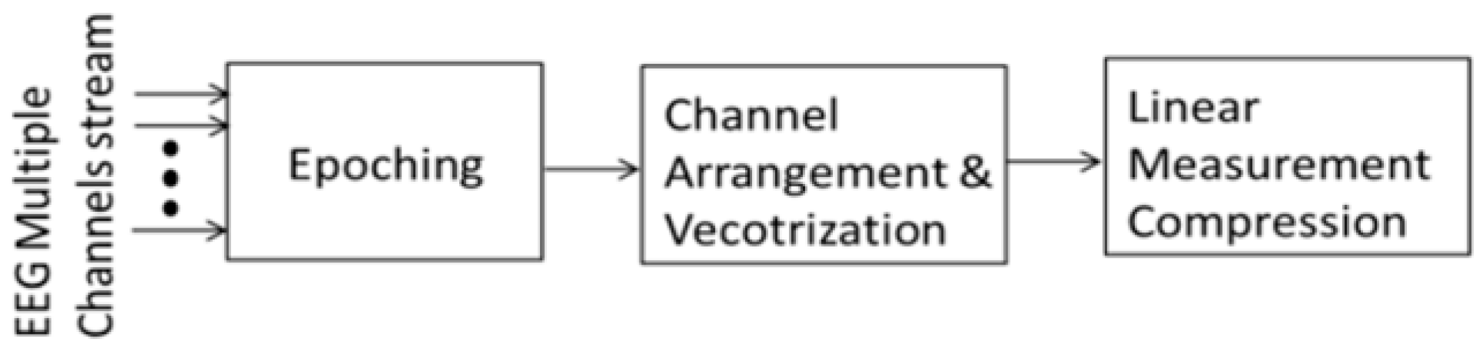
3.2. Implementation
3.2.1. Epoching
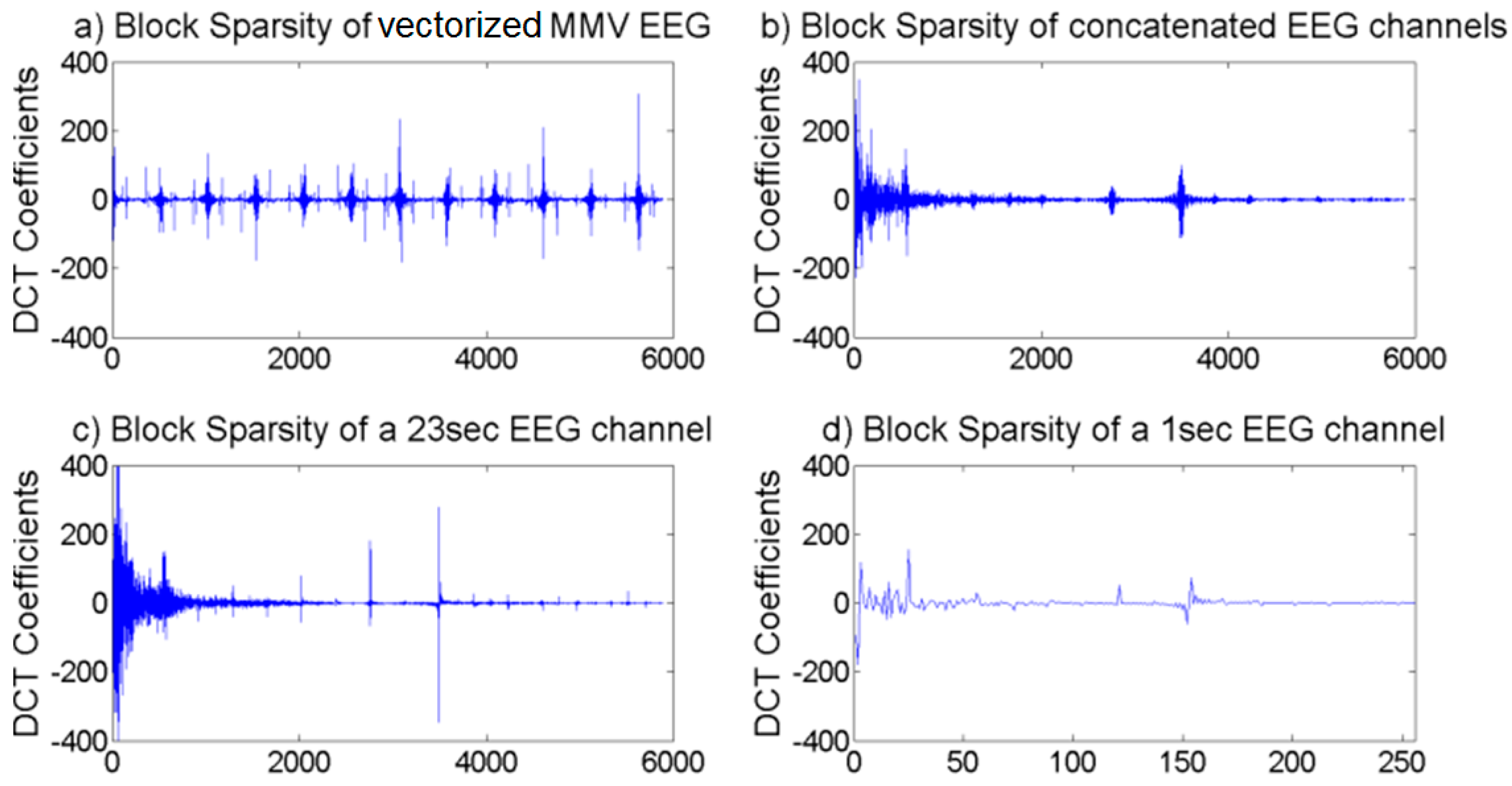
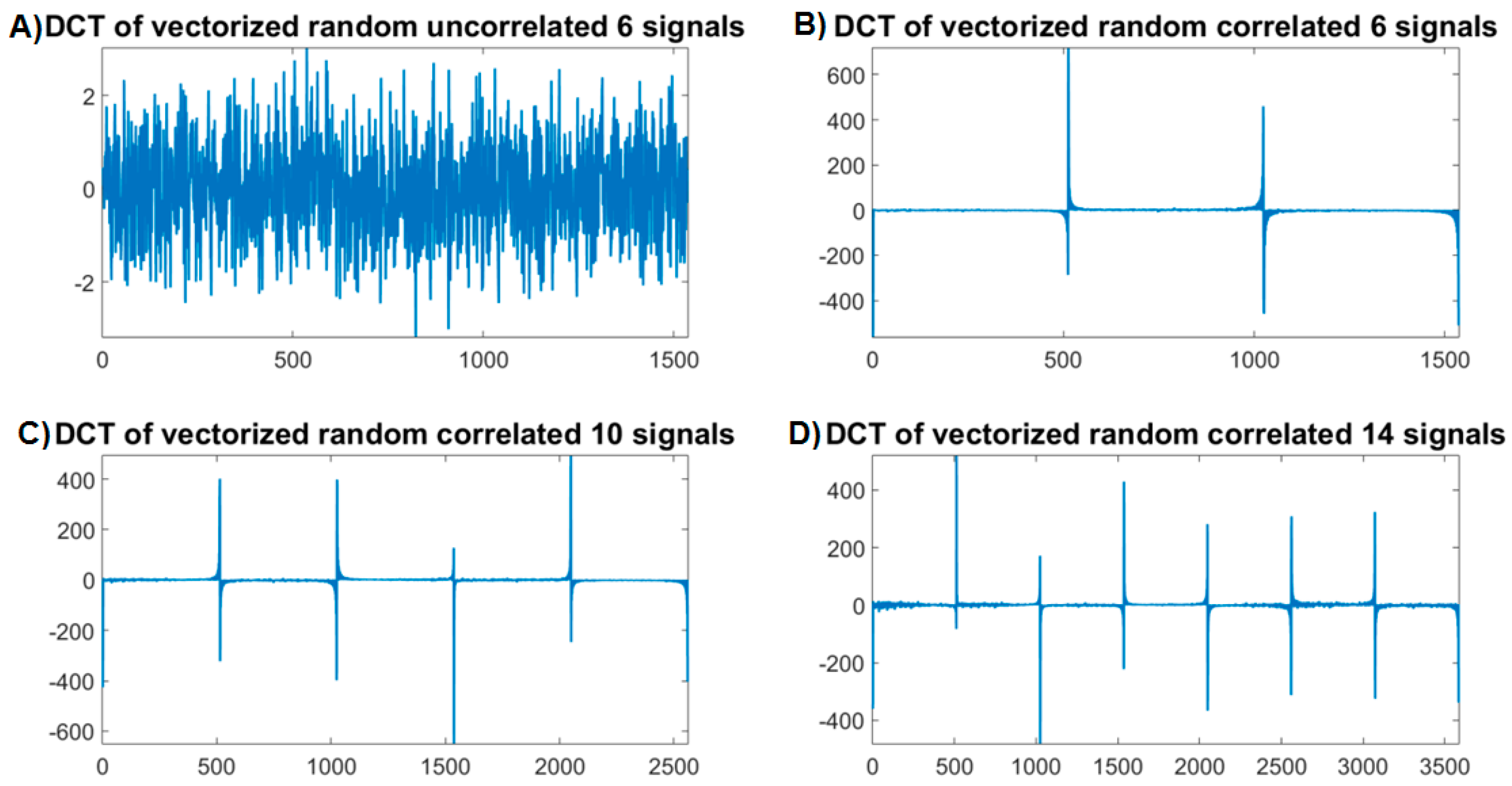
3.2.2. Channel Arrangement and Vectorization

3.2.3. Compression
3.2.4. Modification of BSBL-BO (BSBL-LNLD)
4. Experiments and Results
4.1. Data Set
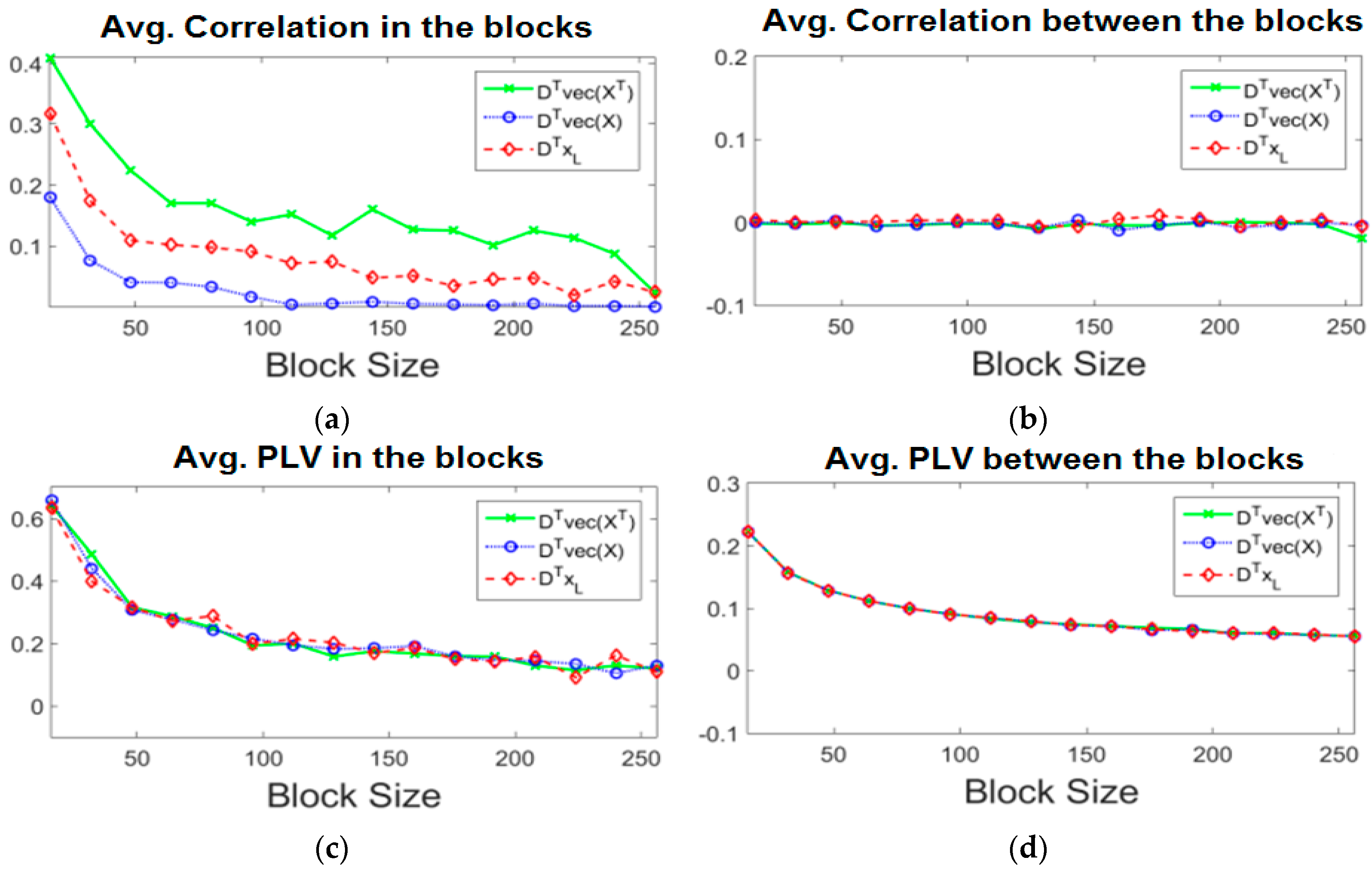
4.2. Dependence Measure of Intra and Inter EEG Blocks

4.3. Error Metrics and Experiements
4.4. Compression/Decompresion Results
- (1)
- The tMFOCUSS proposed in [10] is a modified version of the MFOCUSS. It works by capturing the temporal correlation in the channels. The modification lies in replacing the norm minimization with the Mahalanobis distance.
- (2)
- The TMSBL method proposed in [9]. It is a Bayesian approach. It defines the signal in the hyper-parameter space instead of the Euclidian space such as in l1/l2 minimization techniques. The hyper-parameter space is defined by temporal correlation and sparse modelling, this approach is called the Automatic Relevance Determination as proposed in [9,34]. By using Expected Maximization, the hyper-parameters are estimated from the posterior information, which is derived from a prior and the log-likelihood of the compressed signal. One can argue that TMSBL is similar to BSBL-BO in its basic approach and derivation. However, BSBL-BO reconstructs the signal in blocks form, unlike TMSBL.

- (3)
- Recently, the BSBL-BO approach [1] was compared with the STSBL-EM algorithm presented in [12]. The comparison was performed on BCI data at different compression rates such as 50%, 60%, 70%, 80%, and 90%. It was shown that the decompression of SMV BSBL was less accurate than STSBL-EM. Two learning hyper-parameters were introduced in STSBL-EM, to capture the correlation between the blocks in the temporal and spatial domains. STSBL-EM learns the parameters by temporally whitening the model at first, and then the spatial hyper-parameter is learned and the signals are estimated. Then the signals are spatially whitened and then the temporal hyper-parameter and the signals are estimated. This process repeats until convergence within 2 to 3 s on average. The repetitive whiting of the model reduces the correlation in the signals which causes less redundancy during decompression, hence less correlation amongst the blocks. Our results in the Table 1 show that compared to the other methods STSBL-EM does not achieve low errors at high compression rates.

| CR | 90% | 85% | 80% | 70% | 60% | 50% | |
|---|---|---|---|---|---|---|---|
| Compression Experiment | |||||||
| NMSE (BCI DataSet) | BSBL-LNLD (Multichannel) | 0.065 | 0.058 | 0.016 | 0.008 | 0.005 | 0.002 |
| BSBL-BO (Multichannel) | 0.094 | 0.089 | 0.075 | 0.014 | 0.006 | 0.003 | |
| BSBL-LNLD (SingleChannel) | 0.461 | 0.384 | 0.242 | 0.154 | 0.094 | 0.045 | |
| BSBL-BO (SingleChannel) | 0.551 | 0.414 | 0.318 | 0.217 | 0.134 | 0.089 | |
| STBSL-EM | 0.791 | 0.427 | 0.133 | 0.038 | 0.017 | 0.009 | |
| TMSBL | 0.248 | 0.178 | 0.066 | 0.04 | 0.022 | 0.014 | |
| tMFOCUS | 0.665 | 0.269 | 0.077 | 0.035 | 0.018 | 0.011 | |
| NMSE (Seizure DataSet) | BSBL-LNLD (Multichannel) | 0.242 | 0.191 | 0.174 | 0.114 | 0.097 | 0.035 |
| BSBL-BO (Multichannel) | 0.311 | 0.257 | 0.216 | 0.165 | 0.114 | 0.058 | |
| BSBL-LNLD (SingleChannel) | 0.457 | 0.412 | 0.35 | 0.261 | 0.156 | 0.098 | |
| BSBL-BO (SingleChannel) | 0.671 | 0.575 | 0.472 | 0.319 | 0.228 | 0.147 | |
| STBSL-EM | 0.984 | 0.728 | 0.419 | 0.166 | 0.091 | 0.032 | |
| TMSBL | 0.698 | 0.687 | 0.217 | 0.154 | 0.11 | 0.036 | |
| tMFOCUS | 0.912 | 0.757 | 0.683 | 0.441 | 0.098 | 0.021 | |
| NMSE (Sleep DataSet) | BSBL-LNLD (Multichannel) | 0.148 | 0.135 | 0.095 | 0.064 | 0.009 | 0.004 |
| BSBL-BO (Multichannel) | 0.176 | 0.153 | 0.113 | 0.094 | 0.015 | 0.007 | |
| BSBL-LNLD (SingleChannel) | 0.388 | 0.265 | 0.147 | 0.092 | 0.058 | 0.029 | |
| BSBL-BO (SingleChannel) | 0.475 | 0.356 | 0.225 | 0.134 | 0.075 | 0.044 | |
| STBSL-EM | 0.89 | 0.561 | 0.315 | 0.126 | 0.065 | 0.007 | |
| TMSBL | 0.352 | 0.243 | 0.156 | 0.114 | 0.072 | 0.009 | |
| tMFOCUS | 0.864 | 0.587 | 0.413 | 0.324 | 0.054 | 0.017 | |
4.5. Power Consumption Simulation
| CR | MCU | Transmitter | Memory | Total (mW) | Battery Life hrs (3V, 200 mAh) |
|---|---|---|---|---|---|
| 0% (No Compression) | 46.14 | 160.68 | 0 | 20.82 | 3.04 |
| 50% | 20.07 | 30.67 | 13.60 | 64.34 | 9.79 |
| 60% | 19.24 | 20.58 | 13.25 | 53.07 | 11.87 |
| 70% | 18.41 | 14.1 | 12.91 | 45.42 | 13.87 |
| 80% | 17.72 | 9.65 | 12.76 | 40.14 | 15.69 |
| 90% | 17.04 | 6.67 | 12.78 | 36.49 | 17.27 |
5. Conclusions and Future Work
Acknowledgments
Author Contributions
Conflicts of Interest
References
- Zhang, Z.; Jung, T.-P.; Makeig, S.; Rao, B.D. Compressed Sensing of EEG for Wireless Telemonitoring with Low Energy Consumption and Inexpensive Hardware. IEEE Trans. Biomed. Eng. 2014, 60, 221–224. [Google Scholar] [CrossRef] [PubMed]
- Aviyente, S. Compressed Sensing Framework for EEG Compression. In Proceedings of the IEEE/SP 14th Workshop on Statistical Signal Processing, Madison, WI, USA, 26–29 August 2007; pp. 181–184.
- Abdulghani, A.M.; Casson, A.J.; Rodriguez-Villegas, E. Quantifying the performance of compressive sensing on scalp EEG signals. In Proceedings of the 3rd International Symposium on Applied Sciences in Biomedical and Communication Technologies (ISABEL), Rome, Italy, 7–10 November 2010; pp. 1–5.
- Mamaghanian, H.; Khaled, N.; Atienza, D.; Vandergheynst, P. Compressed sensing for real-time energy-efficient ECG compression on wireless body sensor nodes. IEEE Trans. Biomed. Eng. 2011, 58, 2456–2466. [Google Scholar] [CrossRef] [PubMed]
- Candes, E.; Wakin, M. An introduction to compressive sampling. IEEE Signal Process. Mag. 2008, 25, 21–30. [Google Scholar] [CrossRef]
- Fauvel, S.; Ward, R.K. An Energy Efficient Compressed Sensing Framework for the Compression of Electroencephalogram Signals. Sensors 2014, 14, 1474–1496. [Google Scholar] [CrossRef] [PubMed]
- Zhang, H.; Chen, C.; Wu, Y.; Li, P. Decomposition and compression for ECG and EEG signals with sequence index coding method based on matching pursuit. J. China Univ. Posts Telecommun. 2012, 19, 92–95. [Google Scholar] [CrossRef]
- Mijovic, B.; Matic, V.; de Vos, M.; van Huffel, S. Independent component analysis as a preporocessing step for data compression of neonatal EEG. In Proceedings of the Annual International Conference of the IEEE Engineering Medicine and Biology Society, Boston, MA, USA, 30 August–3 September 2011; pp. 7316–7319.
- Zhang, Z.; Rao, B.D. Iterative Reweighted Algorithms for Sparse Signal Recovery with Temporally Correlated Source Vectors. In Proceedings of the IEEE International Conference on Acoustics, Speech and Signal Processing, Prague, Czech Republic, 22–27 May 2011.
- Zhang, Z.; Rao, B.D. Sparse Signal Recovery with Temporally Correlated Source Vectors Using Sparse Bayesian Learning. IEEE J. Sel. Top. Signal Process. 2011, 5, 912–926. [Google Scholar] [CrossRef]
- Cotter, S.F.; Rao, B.D.; Kjersti, E.; Kreutz-Delgado, K. Sparse solutions to linear inverse problems with multiple measurement vectors. IEEE Trans. Signal Process. 2005, 53, 2477–2488. [Google Scholar] [CrossRef]
- Zhang, Z.; Jung, T.-P.; Makeig, S.; Pi, Z.; Rao, B.D. Spatiotemporal Sparse Bayesian Learning with Applications to Compressed Sensing of Multichannel Physiological Signals. IEEE Trans. Neural Syst. Rehabil. Eng. 2014, 22, 1186–1197. [Google Scholar] [CrossRef] [PubMed]
- Ward, R.K.; Majumdar, A. Energy efficient EEG sensing and transmission for wireless body area networks: A blind compressed sensing approach. Biomed. Signal Process. Control 2015, 20, 1–9. [Google Scholar]
- Ward, R.K.; Majumdar, A.; Gogna, A. Low-rank matrix recovery approach for energy efficient EEG acquisition for wireless body area network. Sensors 2014, 14, 15729–15748. [Google Scholar]
- Majumdar, A.; Shukla, A. Row-sparse blind compressed sensing for reconstructing multi-channel EEG signals. Biomed. Signal Process. Control 2015, 18, 174–178. [Google Scholar]
- Blankertz, B.; Dornhege, G.; Krauledat, M.; Mller, K.; Curio, G. The non-invasive berlin brain-computer interface: Fast acquisition of effective performance in untrained subjects. NeuroImage 2007, 37, 539–550. [Google Scholar] [CrossRef] [PubMed]
- Gevins, A.S.; Cutillo, B.A. Neuroelectric measures of mind. In Neocortical Dynamics and Human EEG Rhythms; Oxford University Press: New York, NY, USA, 1995; pp. 304–338. [Google Scholar]
- Katznelson, R.D. Normal modes of the brain: Neuroanatomical basis and a physiological theoretical model. In Electric Fields of the Brain: The Neurophysics of EEG, 1st ed.; Oxford University Press: New York, NY, USA, 1981; pp. 401–442. [Google Scholar]
- Breakspear, M.; Terry, J.R. Detection and description of non-linear interdependence in normal multichannel human EEG data. Clin. Neurophysiol. 2002, 113, 735–753. [Google Scholar] [CrossRef]
- Pereda, E.; Quian, R.Q.; Bhattacharya, J. Nonlinear multivariate analysis of neurophysiological signals. Prog. Neurobiol. 2005, 77, 1–37. [Google Scholar] [CrossRef] [PubMed]
- Herrmann, F.J. Randomized sampling and sparsity: Getting more information from fewer samples. Geophysics 2010, 75. [Google Scholar] [CrossRef]
- Mallat, S.G. A Wavelet Tour of Signal Processing, 3rd ed.; Academic Press: New York, NY, USA, 2008. [Google Scholar]
- Herrmann, F.J.; Friedlander, M.P.; Yilmaz, O. Fighting the curse of dimensionality: Compressive sensing in exploration seismology. IEEE Signal Process. Mag. 2011, 29, 88–100. [Google Scholar] [CrossRef]
- Zhang, Z.; Rao, B.D. Extension of SBL Algorithms for the Recovery of Block Sparse Signals with Intra-Block Correlation. IEEE Trans. Signal Process. 2013, 61, 2009–2015. [Google Scholar] [CrossRef]
- Eldar, Y.C.; Kuppinger, P.; Bolcskei, H. Block-Sparse Signals: Uncertainty Relations and Efficient Recovery. IEEE Trans. Signal Process. 2010, 58, 3042–3054. [Google Scholar] [CrossRef]
- Eldar, Y.C.; Mishali, M. Block sparsity and sampling over a union of subspaces. In Proceedings of the 16th International Conference on Digital Signal Processing, Santorini, Greece, 5–7 July 2009; pp. 1–8.
- Eldar, Y.C.; Mishali, M. Robust recovery of signals from a structured union of subspaces. IEEE Trans. Inf. Theory 2009, 55, 5302–5316. [Google Scholar] [CrossRef]
- Chen, J.; Huo, X. Theoretical results on sparse representations of multiple-measurement vectors. IEEE Trans. Signal Process. 2006, 54, 4634–4643. [Google Scholar] [CrossRef]
- Duarte, M.F.; Sarvotham, S.; Wakin, M.B.; Baron, D.; Baraniuk, R.G. Joint Sparsity Models for Distributed Compressed Sensing. In Proceedings of the Workshop on Signal Processing with Adaptive Sparse Structured Representations, Rennes, France, 16–18 November 2005.
- Zhang, Z.; Rao, B.D. Sparse signal recovery in the presence of correlated multiple measurement vectors. In Proceedings of the IEEE International Conference on Acoustics, Speech and Signal Processing (ICASSP), Dallas, TX, USA, 14–19 March 2010.
- Lachaux, J.P.; Rodriguez, E.; Martinerie, J.; Varela, F.J. Measuring phase synchrony in brain signals. Hum. Brain Map. 1999, 8, 194–208. [Google Scholar] [CrossRef]
- Terzano, M.G.; Parrino, L.; Sherieri, A.; Chervin, R.; Chokroverty, S.; Guilleminault, C.; Hirshkowitz, M.; Mahowald, M.; Moldofsky, H.; Rosa, A.; et al. Atlas, rules, and recording techniques for the scoring of cyclic alternating pattern (CAP) in human sleep. Sleep Med. 2001, 2, 537–553. [Google Scholar] [CrossRef]
- Goldberger, A.L.; Amaral, L.A.N.; Glass, L.; Hausdorff, J.M.; Ivanov, P.C.; Mark, R.G.; Mietus, J.E.; Moody, G.B.; Peng, C.-K.; Stanley, H.E. PhysioBank, PhysioToolkit, and PhysioNet: Components of a New Research Resource for Complex Physiologic Signals. Circulation 2000, 101, e215–e220. [Google Scholar] [CrossRef] [PubMed]
- Michael, E. Tipping: Sparse Bayesian Learning and the Relevance Vector Machine. J. Mach. Learn. Res. 2001, 1, 211–244. [Google Scholar]
- Palsberg, J.; Titzer, B.L.; Lee, D.K. Avrora: Scalable sensor network simulation with precise timing. In Proceedings of the Fourth International Symposium on Information Processing in Sensor Networks, Los Angeles, CA, USA, 25–27 April 2005.
- Levis, P.; Madden, S.; Polastre, J.; Szewczyk, R.; Whitehouse, K.; Woo, A.; Gay, D.; Hill, J.; Welsh, M.; Brewer, E.; et al. Tinyos: An operating system for sensor networks. In Ambient Intelligence; Springer: New York, NY, USA, 2005. [Google Scholar]
- Yazicioglu, R.F.; Torfs, T.; Merken, P.; Penders, J.; Leonov, V.; Puers, R.; Gyselinckx, B.; van Hoof, C. Ultra-low-power biopotential interfaces and their applications in wearable and implantable systems. Microelectron. J. 2009, 40, 1313–1321. [Google Scholar] [CrossRef]
© 2016 by the authors; licensee MDPI, Basel, Switzerland. This article is an open access article distributed under the terms and conditions of the Creative Commons by Attribution (CC-BY) license (http://creativecommons.org/licenses/by/4.0/).
Share and Cite
Mahrous, H.; Ward, R. Block Sparse Compressed Sensing of Electroencephalogram (EEG) Signals by Exploiting Linear and Non-Linear Dependencies. Sensors 2016, 16, 201. https://doi.org/10.3390/s16020201
Mahrous H, Ward R. Block Sparse Compressed Sensing of Electroencephalogram (EEG) Signals by Exploiting Linear and Non-Linear Dependencies. Sensors. 2016; 16(2):201. https://doi.org/10.3390/s16020201
Chicago/Turabian StyleMahrous, Hesham, and Rabab Ward. 2016. "Block Sparse Compressed Sensing of Electroencephalogram (EEG) Signals by Exploiting Linear and Non-Linear Dependencies" Sensors 16, no. 2: 201. https://doi.org/10.3390/s16020201
APA StyleMahrous, H., & Ward, R. (2016). Block Sparse Compressed Sensing of Electroencephalogram (EEG) Signals by Exploiting Linear and Non-Linear Dependencies. Sensors, 16(2), 201. https://doi.org/10.3390/s16020201