
Images from Bits: Non-Iterative Image Reconstruction for Quanta Image Sensors


Abstract
:
1. Introduction
1.1. Quanta Image Sensor
1.2. Scope and Contribution
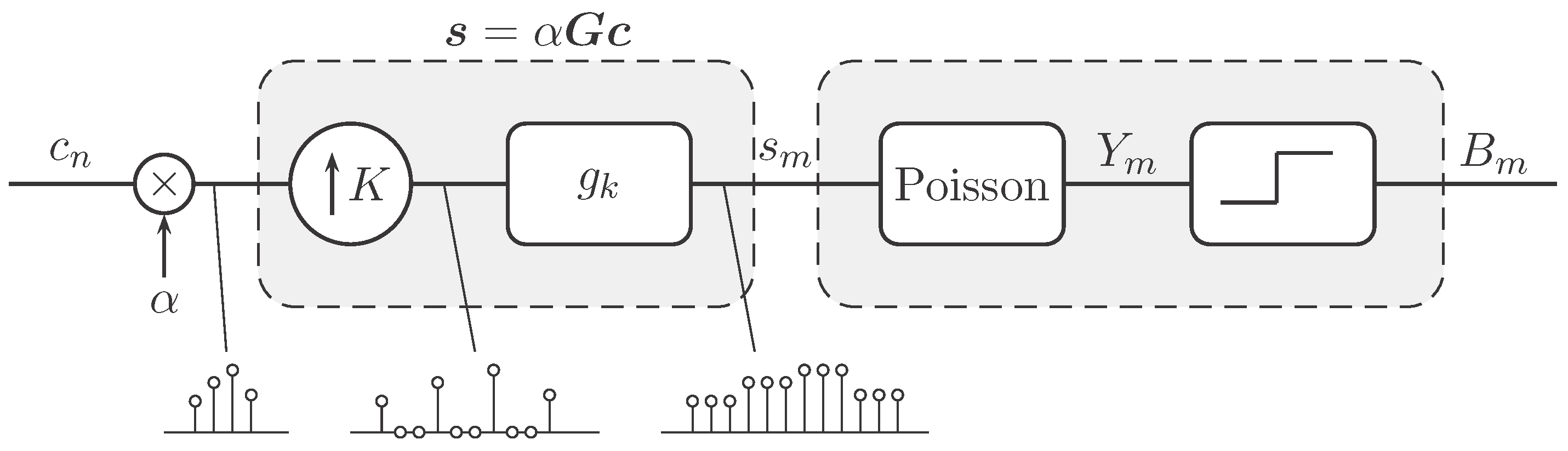
2. QIS Imaging Model
2.1. Oversampling Mechanism
2.2. Quantized Poisson Observation
2.3. Image Reconstruction for QIS
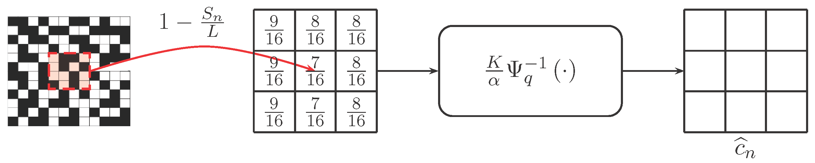
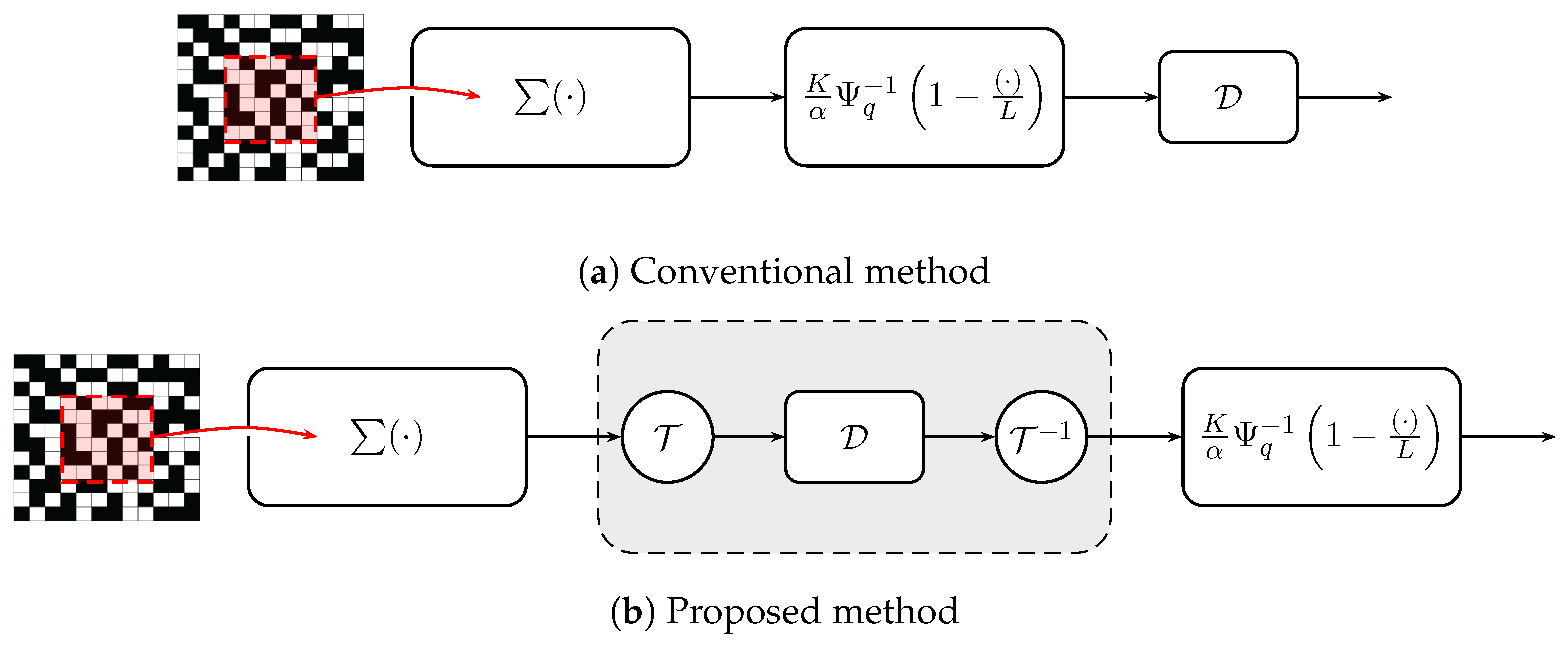
3. Non-Iterative Image Reconstruction
3.1. Component 1: Approximate MLE
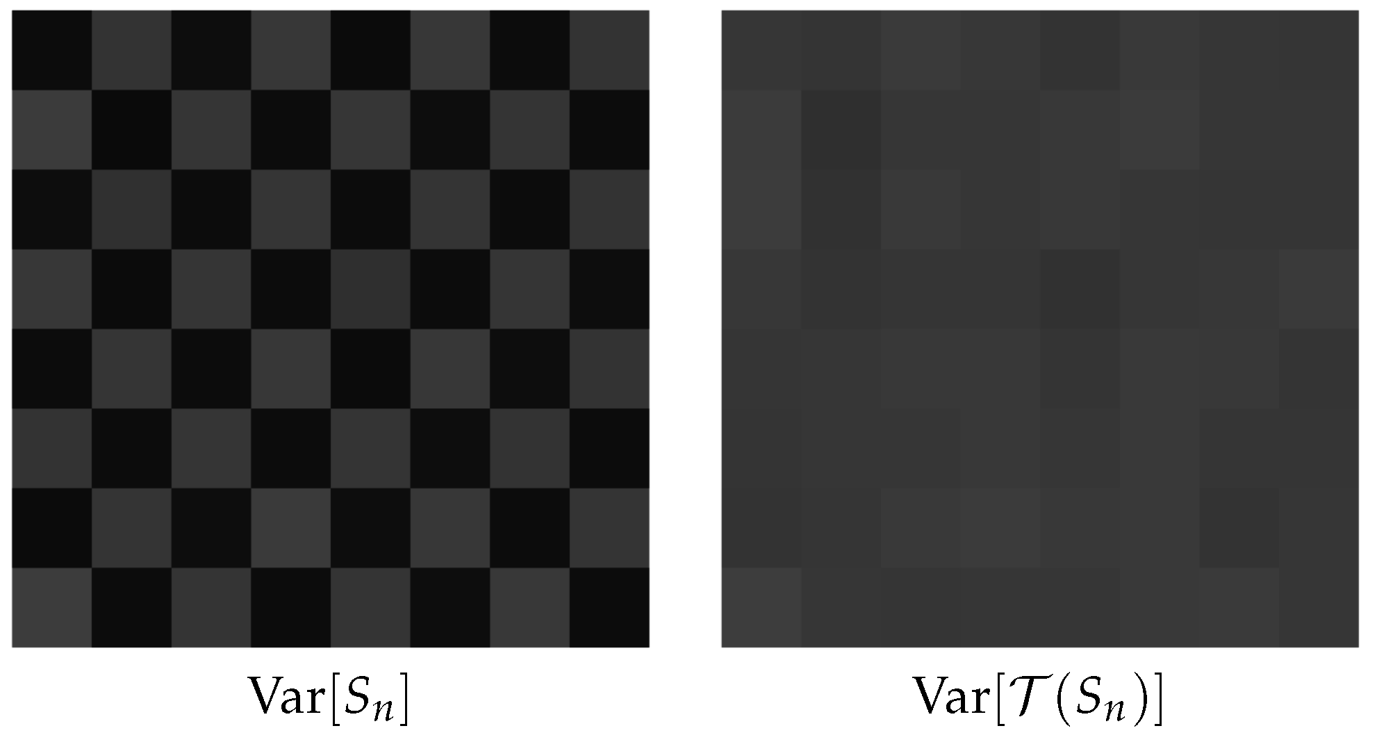
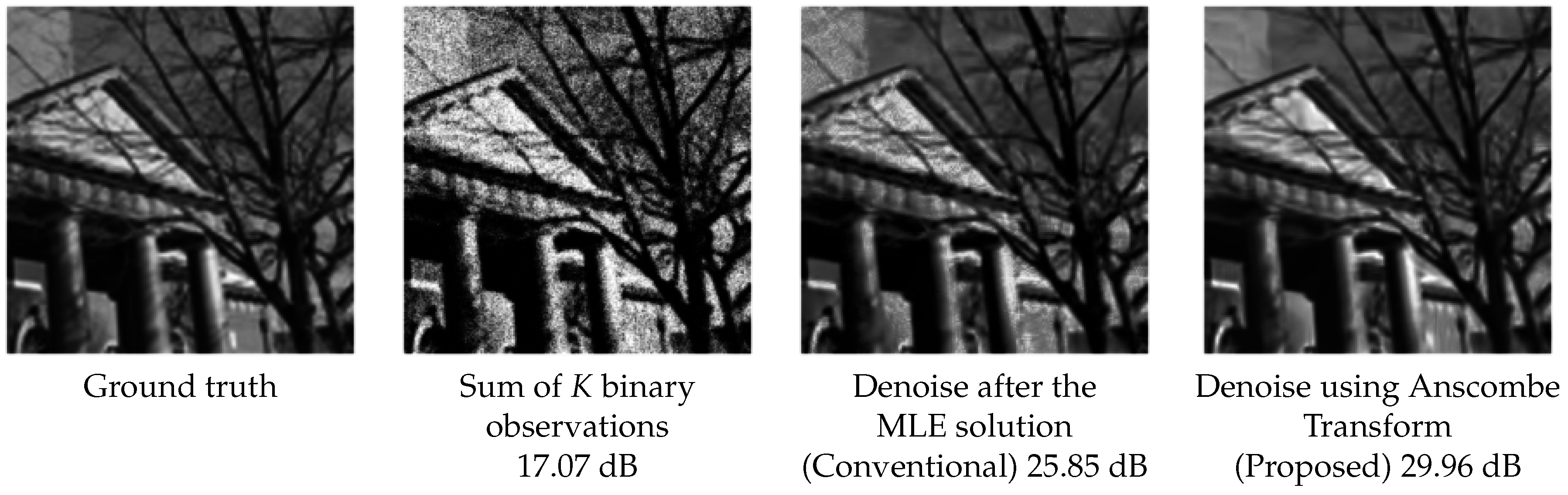
3.2. Component 2: Anscombe Transform
3.3. Component 3: Image Denoiser
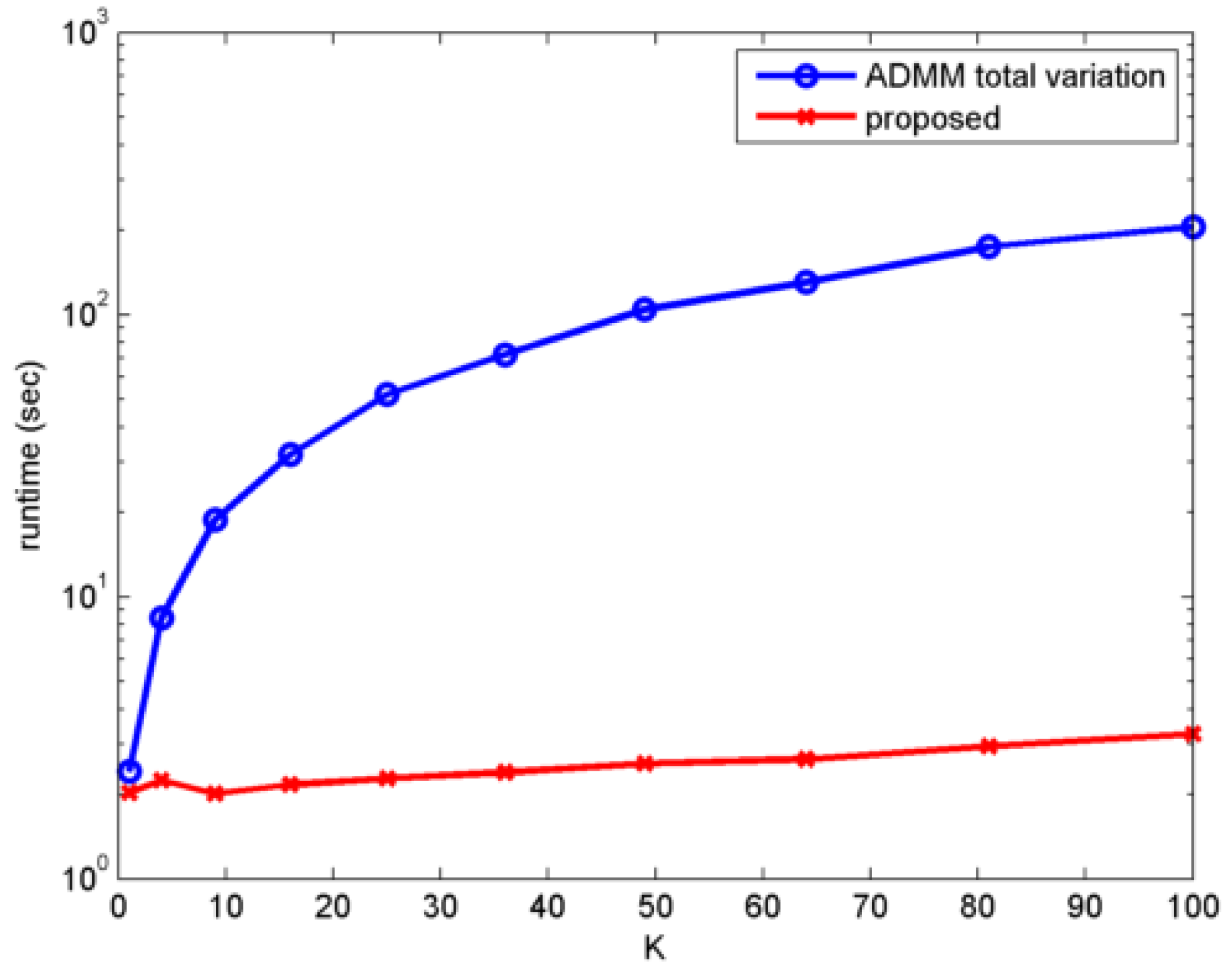
- Total variation denoising [34]: Total variation denoising was originally proposed by Rudin, Osher and Fatemi [34], although other researchers had proposed similar methods around the same time [41]. Total variation denoising formulates the denoising problem as an optimization problem with a total variation regularization. Total variation denoising can be performed very efficiently using the alternating direction method of multipliers (ADMM), e.g., [42,43,44].
- Bilateral filter [45]: The bilateral filter is a nonlinear filter that denoises the image using a weighted average operator. The weights in a bilateral filter are the Euclidean distance between the intensity values of two pixels, plus the spatial distance between the two pixels. A Gaussian kernel is typically employed for these distances to ensure proper decaying of the weights. Bilateral filters are extremely popular in computer graphics for applications, such as detail enhancement. Various fast implementations of bilateral filters are available, e.g., [46,47].
- Non-local Means [48]: non-local means (NLM) was proposed by Buades et al. [48] and, also, an independent work of Awante and Whitaker [49]. Non-local means (NLM) is an extension of the bilateral filter where the Euclidean distance is computed from a small patch instead of a pixel. Experimentally, it has been widely agreed that such patch-based approaches are very effective for image denoising. Fast NLM implementations are now available [50,51,52].
- BM3D [53]: 3D block matching (BM3D) follows the same idea of non-local means by considering patches. However, instead of computing the weighted average, BM3D groups similar patches to form a 3D stack. By applying a 3D Fourier transform (or any other frequency domain transforms, e.g., discrete cosine transform), the commonality of the patches will demonstrate a group sparse behavior in the transformed domain. Thus, by applying a threshold in the transformed domain, one can remove the noise very effectively. BM3D is broadly regarded as a benchmark of today’s image denoising algorithm.
3.4. Related Work in the Literature
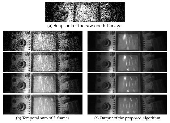
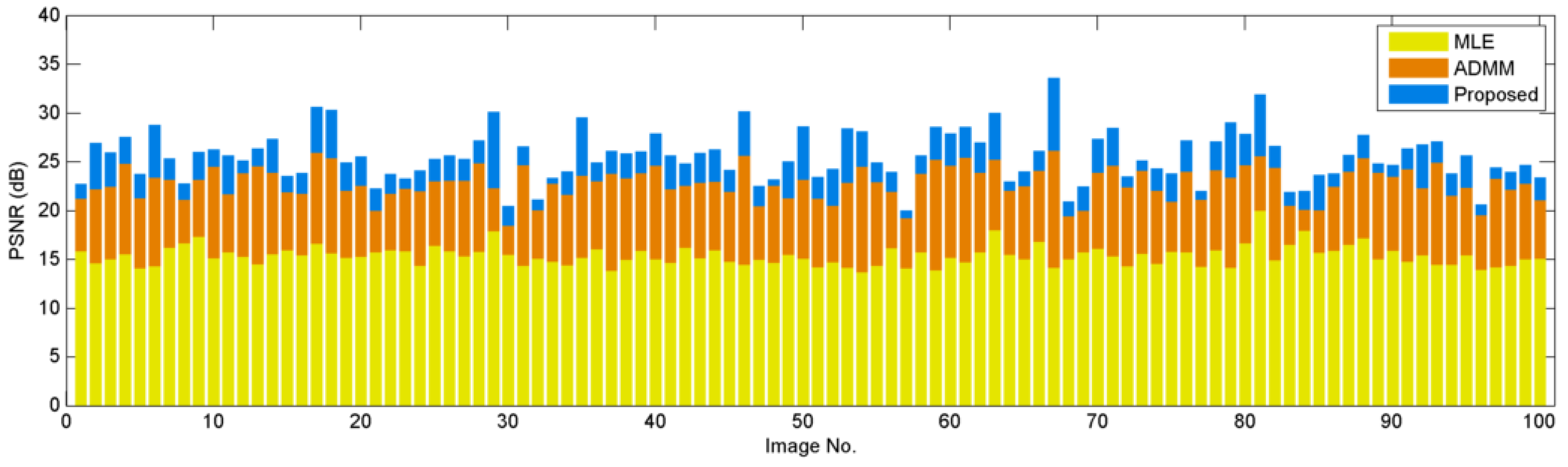
4. Experimental Results
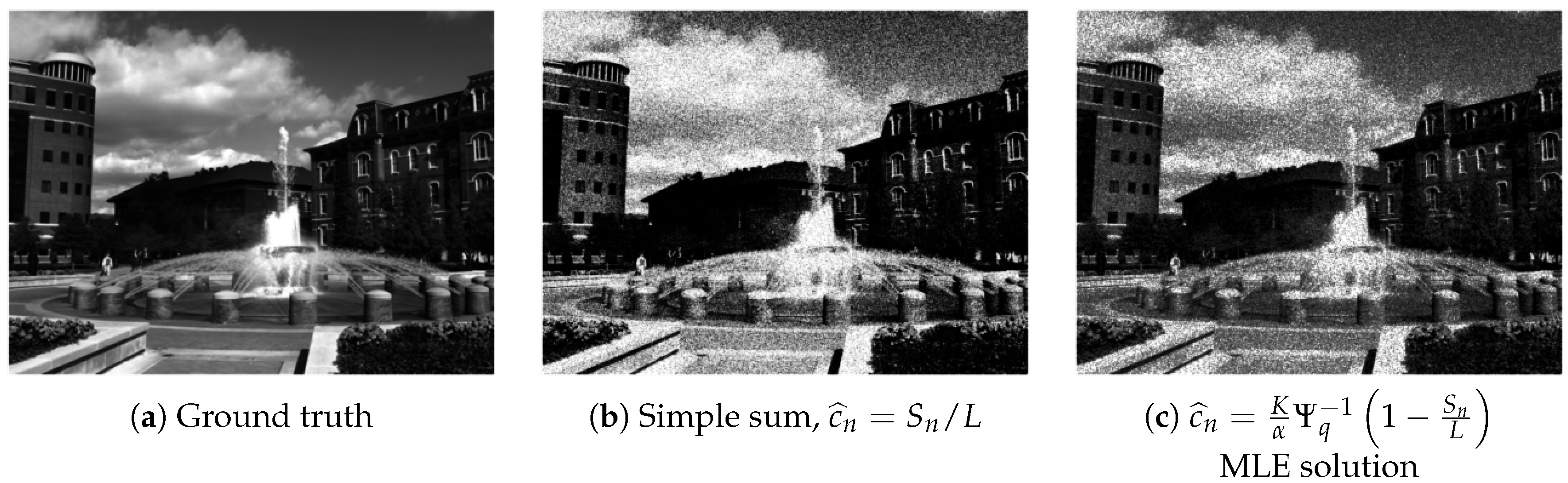
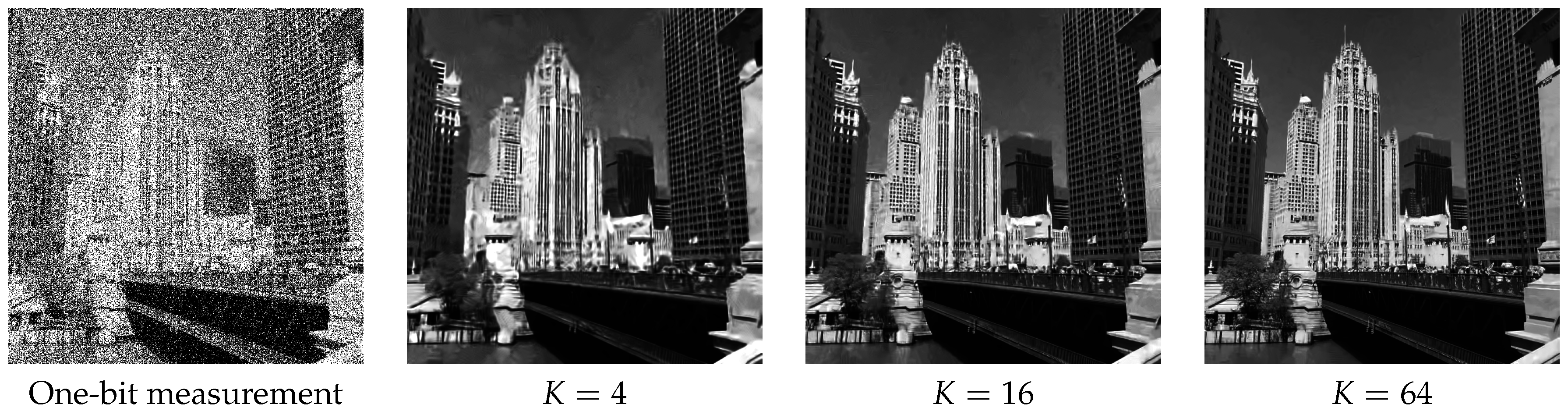
4.1. Synthetic Data
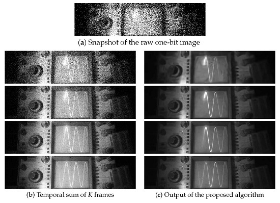
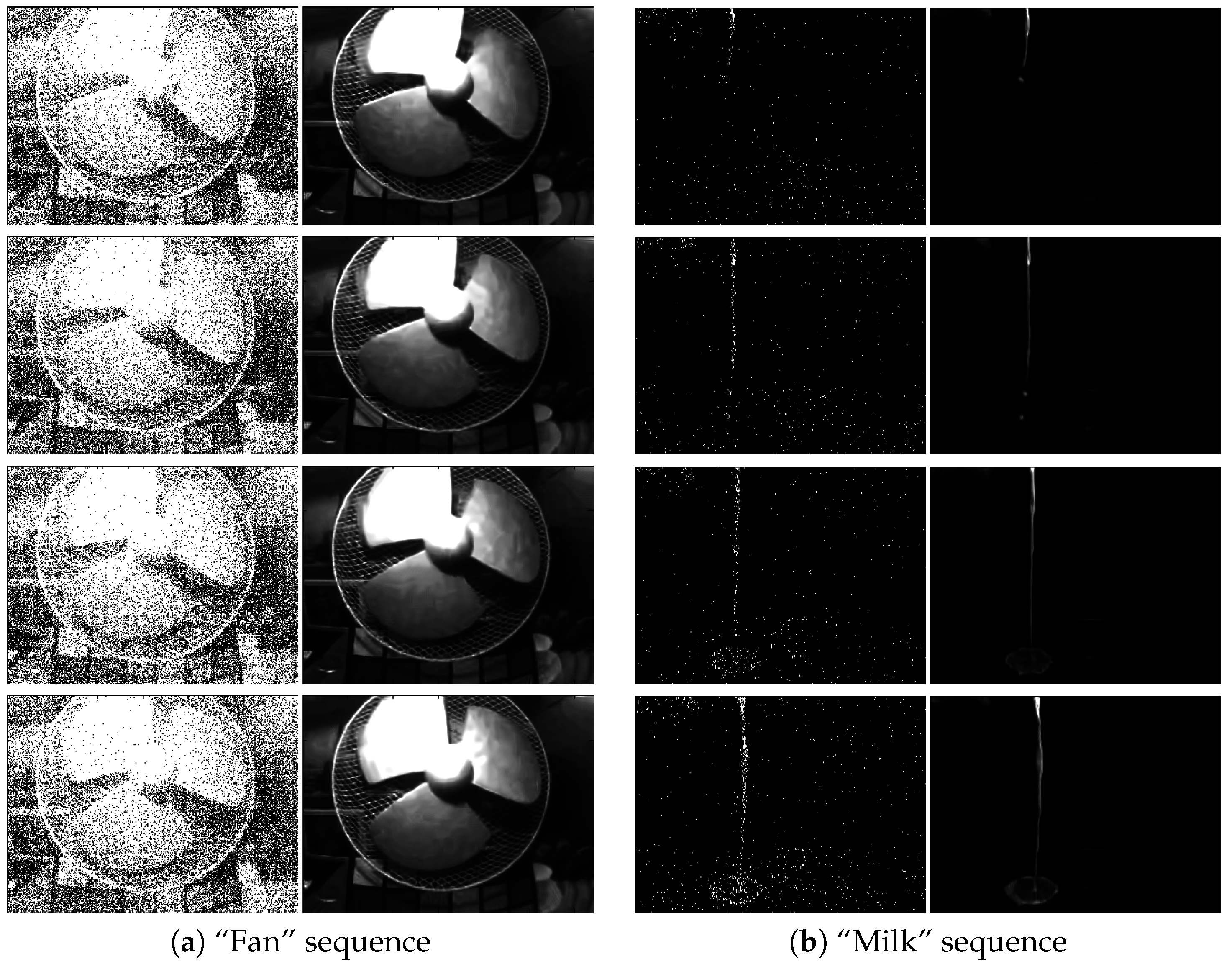
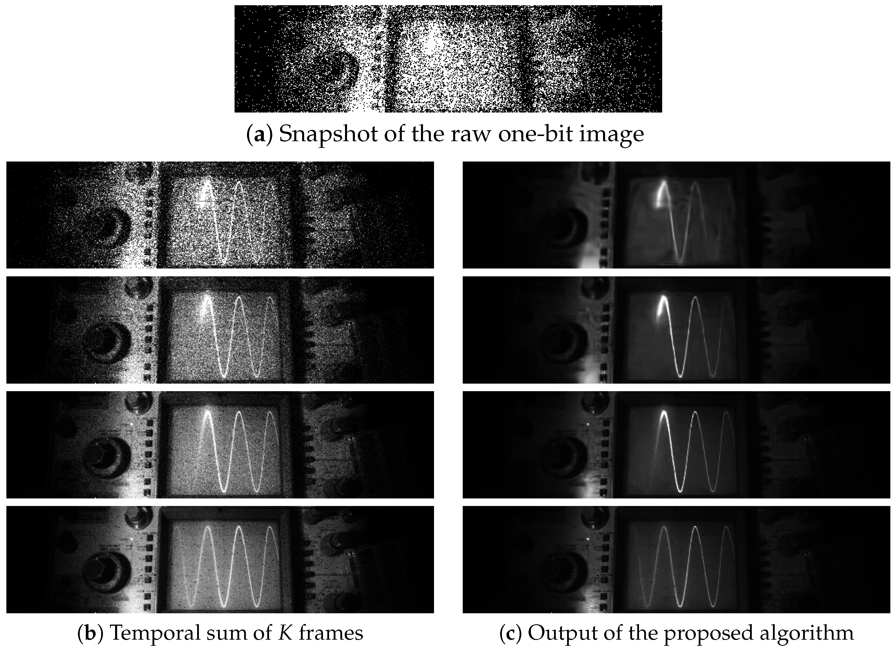
4.2. Real Data
5. Conclusions
Acknowledgments
Author Contributions
Conflicts of Interest
Abbreviations
| CCD | Charge coupled device |
| CMOS | Complementary metal-oxide-semiconductor |
| QIS | Quanta image sensors |
| MLE | Maximum likelihood estimation |
| ADMM | Alternating direction method of multipliers |
| SPAD | Single-photon avalanche diode |
| PSNR | Peak signal to noise ratio |
| BM3D | 3D block matching |
| i.i.d. | Independently and identically distributed |
Appendix A
Appendix A.1. Proof of Proposition 1
Appendix A.2. Proof of Theorem 1
References
- Press Release of Nobel Prize 2009. Available online: http://www.nobelprize.org/nobel_prizes/physics/laureates/2009/press.html (accessed on 18 November 2016).
- Fossum, E.R. Active Pixel Sensors: Are CCD’s Dinosaurs? Proc. SPIE 1993, 1900, 2–14. [Google Scholar]
- Clark, R.N. Digital Camera Reviews and Sensor Performance Summary. Available online: http://www.clarkvision.com/articles/digital.sensor.performance.summary (accessed on 18 November 2016).
- Fossum, E.R. Some Thoughts on Future Digital Still Cameras. In Image Sensors Signal Processing for Digital Still Cameras; Nakamura, J., Ed.; CRC Press: Boca Raton, FL, USA, 2005; Chapter 11; pp. 305–314. [Google Scholar]
- Fossum, E.R. What to do with sub-diffraction-limit (SDL) pixels?—A proposal for a gigapixel digital film sensor (DFS). In Proceedings of the IEEE Workshop Charge-Coupled Devices and Advanced Image Sensors, Nagano, Japan, 9–11 June 2005; pp. 214–217.
- Fossum, E.R. The Quanta Image Sensor (QIS): Concepts and Challenges. In OSA Technical Digest (CD), Paper JTuE1, Proceedings of the OSA Topical Mtg on Computational Optical Sensing and Imaging, Toronto, ON, Canada, 10–14 July 2011; Optical Society of America: Washington, DC, USA, 2011. [Google Scholar]
- Masoodian, S.; Song, Y.; Hondongwa, D.; Ma, J.; Odame, K.; Fossum, E.R. Early research progress on quanta image sensors. In Proceedings of the International Image Sensor Workshop (IISW), Snowbird, UT, USA, 12–16 June 2013.
- Ma, J.; Fossum, E.R. Quanta image sensor jot with sub 0.3 e− r.m.s. read noise and photon counting capability. IEEE Electron Device Lett. 2015, 36, 926–928. [Google Scholar] [CrossRef]
- Masoodian, S.; Rao, A.; Ma, J.; Odame, K.; Fossum, E.R. A 2.5 pJ/b binary image sensor as a pathfinder for quanta image sensors. IEEE Trans. Electron Devices 2016, 63, 100–105. [Google Scholar] [CrossRef]
- Fossum, E.R.; Ma, J.; Masoodian, S. Quanta image sensor: Concepts and progress. Proc. SPIE Adv. Photon Count. Tech. X 2016, 9858, 985804. [Google Scholar]
- Sbaiz, L.; Yang, F.; Charbon, E.; Susstrunk, S.; Vetterli, M. The gigavision camera. In Proceedings of the 2009 IEEE International Conference on Acoustics, Speech and Signal Processing (ICASSP), Taipei, Taiwan, 19–24 April 2009; pp. 1093–1096.
- Yang, F.; Sbaiz, L.; Charbon, E.; Süsstrunk, S.; Vetterli, M. On pixel detection threshold in the gigavision camera. Proc. SPIE 2010, 7537. [Google Scholar] [CrossRef]
- Yang, F.; Lu, Y.M.; Sbaiz, L.; Vetterli, M. Bits from photons: Oversampled image acquisition using binary Poisson statistics. IEEE Trans. Image Process. 2012, 21, 1421–1436. [Google Scholar] [CrossRef] [PubMed]
- Dutton, N.A.W.; Parmesan, L.; Holmes, A.J.; Grant, L.A.; Henderson, R.K. 320 × 240 oversampled digital single photon counting image sensor. In Proceedings of the IEEE Symposium VLSI Circuits Digest of Technical Papers, Honolulu, HI, USA, 9–13 June 2014; pp. 1–2.
- Dutton, N.A.W.; Gyongy, I.; Parmesan, L.; Henderson, R.K. Single photon counting performance and noise analysis of CMOS SPAD-based image sensors. Sensors 2016, 16, 1122. [Google Scholar] [CrossRef] [PubMed]
- Dutton, N.A.W.; Gyongy, I.; Parmesan, L.; Gnecchi, S.; Calder, N.; Rae, B.R.; Pellegrini, S.; Grant, L.A.; Henderson, R.K. A SPAD-based QVGA image sensor for single-photon counting and quanta imaging. IEEE Trans. Electron Devices 2016, 63, 189–196. [Google Scholar] [CrossRef]
- Burri, S.; Maruyama, Y.; Michalet, X.; Regazzoni, F.; Bruschini, C.; Charbon, E. Architecture and applications of a high resolution gated SPAD image sensor. Opt. Express 2014, 22, 17573–17589. [Google Scholar] [CrossRef] [PubMed]
- Antolovic, I.M.; Burri, S.; Hoebe, R.A.; Maruyama, Y.; Bruschini, C.; Charbon, E. Photon-counting arrays for time-resolved imaging. Sensors 2016, 16, 1005. [Google Scholar] [CrossRef] [PubMed]
- Vogelsang, T.; Stork, D.G. High-dynamic-range binary pixel processing using non-destructive reads and variable oversampling and thresholds. In Proceedings of the 2012 IEEE Sensors, Taipei, Taiwan, 28–31 October 2012; pp. 1–4.
- Vogelsang, T.; Guidash, M.; Xue, S. Overcoming the full well capacity limit: High dynamic range imaging using multi-bit temporal oversampling and conditional reset. In Proceedings of the International Image Sensor Workshop, Snowbird, UT, USA, 16 June 2013.
- Vogelsang, T.; Stork, D.G.; Guidash, M. Hardware validated unified model of multibit temporally and spatially oversampled image sensor with conditional reset. J. Electron. Imaging 2014, 23, 013021. [Google Scholar] [CrossRef]
- Figueiredo, M.A.T.; Bioucas-Dias, J.M. Restoration of Poissonian images using alternating direction optimization. IEEE Trans. Image Process. 2010, 19, 3133–3145. [Google Scholar] [CrossRef] [PubMed]
- Harmany, Z.T.; Marcia, R.F.; Willet, R.M. This is SPIRAL-TAP: Sparse Poisson intensity reconstruction algorithms: Theory and practice. IEEE Trans. Image Process. 2011, 21, 1084–1096. [Google Scholar] [CrossRef] [PubMed]
- Makitalo, M.; Foi, A. Optimal inversion of the generalized Anscombe transformation for Poisson–Gaussian noise. IEEE Trans. Image Process. 2013, 22, 91–103. [Google Scholar] [CrossRef] [PubMed]
- Salmon, J.; Harmany, Z.; Deledalle, C.; Willet, R. Poisson noise reduction with non-local PCA. J. Math Imaging Vis. 2014, 48, 279–294. [Google Scholar] [CrossRef]
- Rond, A.; Giryes, R.; Elad, M. Poisson inverse problems by the Plug-and-Play scheme. J. Visual Commun. Image Represent. 2016, 41, 96–108. [Google Scholar] [CrossRef]
- Azzari, L.; Foi, A. Variance stabilization for noisy+estimate combination in iterative Poisson denoising. IEEE Signal Process. Lett. 2016, 23, 1086–1090. [Google Scholar] [CrossRef]
- Yang, F.; Lu, Y.M.; Sbaiz, L.; Vetterli, M. An optimal algorithm for reconstructing images from binary measurements. Proc. SPIE 2010, 7533, 75330K. [Google Scholar]
- Chan, S.H.; Lu, Y.M. Efficient image reconstruction for gigapixel quantum image sensors. In Proceedings of the 2014 IEEE Global Conference on Signal Information Processing (GlobalSIP), Atlanta, GA, USA, 3–5 December 2014; pp. 312–316.
- Remez, T.; Litany, O.; Bronstein, A. A picture is worth a billion bits: Real-time image reconstruction from dense binary threshold pixels. In Prroceedings of the 2016 IEEE International Conference on Computational Photography (ICCP), Evanston, IL, USA, 13–15 May 2016; pp. 1–9.
- Elgendy, O.; Chan, S.H. Image reconstruction and threshold design for quanta image sensors. In Proceedings of the 2016 IEEE International Conference on Image Processing (ICIP), Phoenix, AZ, USA, 25–28 September 2016; pp. 978–982.
- Anscombe, F.J. The transformation of Poisson, binomial and negative-binomial data. Biometrika 1948, 35, 246–254. [Google Scholar] [CrossRef]
- Abramowitz, M.; Stegun, I.A. Handbook of Mathematical Functions with Formulas, Graphs, and Mathematical Tables; Dover Publications: New York, NY, USA, 1965. [Google Scholar]
- Rudin, L.; Osher, S.; Fatemi, E. Nonlinear total variation based noise removal algorithms. Physica D 1992, 60, 259–268. [Google Scholar] [CrossRef]
- Elad, M. Sparse and Redundant Representations; Springer: New York, NY, USA, 2010. [Google Scholar]
- Fossum, E.R.; Ma, J.; Masoodian, S.; Anzagira, L.; Zizza, R. The quanta image sensor: Every photon counts. Sensors 2016, 16, 1260. [Google Scholar] [CrossRef] [PubMed]
- Antolovic, I.M.; Burri, S.; Bruschini, C.; Hoebe, R.; Charbon, E. Nonuniformity analysis of a 65-kpixel CMOS SPAD imager. IEEE Trans. Electron Devices 2016, 63, 57–64. [Google Scholar] [CrossRef]
- Leon-Garcia, A. Probability, Statistics, and Random Processes for Electrical Engineering; Pearson Prentice Hall: Upper Saddle River, NJ, USA, 2008. [Google Scholar]
- Wasserman, L. All of Nonparametric Statistics; Springer: New York, NY, USA, 2006. [Google Scholar]
- Brown, L.; Cai, T.; DasGupta, A. On Selecting a Transformation: With Applications. Available online: http://www.stat.purdue.edu/~dasgupta/vst.pdf (accessed on 18 November 2016).
- Sauer, K.; Bouman, C.A. Bayesian estimation of transmission tomograms using segmentation based optimization. IEEE Trans. Nucl. Sci. 1992, 39, 1144–1152. [Google Scholar] [CrossRef]
- Afonso, M.; Bioucas-Dias, J.; Figueiredo, M. Fast image recovery using variable splitting and constrained optimization. IEEE Trans. Image Process. 2010, 19, 2345–2356. [Google Scholar] [CrossRef] [PubMed]
- Chan, S.H.; Khoshabeh, R.; Gibson, K.B.; Gill, P.E.; Nguyen, T.Q. An augmented Lagrangian method for total variation video restoration. IEEE Trans. Image Process. 2011, 20, 3097–3111. [Google Scholar] [CrossRef] [PubMed]
- Wang, Y.; Yang, Y.; Yin, W.; Zhang, Y. A new alternating minimization algorithm for total variation image reconstruction. SIAM J. Imaging Sci. 2008, 1, 248–272. [Google Scholar] [CrossRef]
- Tomasi, C.; Manduchi, R. Bilateral filtering for gray and color images. In Proceedings of the Sixth International Conference on Computer Vision, Bombay, India, 4–7 January 1998; pp. 839–846.
- Paris, S.; Durand, F. A fast approximation of the bilateral filter using a signal processing approach. Int. J. Comput. Vis. 2009, 81, 24–52. [Google Scholar] [CrossRef]
- Chaudhury, K.N.; Sage, D.; Unser, M. Fast (1) bilateral filtering using trigonometric range kernels. IEEE Trans. Image Process. 2011, 20, 3376–3382. [Google Scholar] [CrossRef] [PubMed]
- Buades, A.; Coll, B.; Morel, J.M. A non-local algorithm for image denoising. In Proceedings of the IEEE Computer Society Conference on Computer Vision and Pattern Recognition (CVPR), San Diego, CA, USA, 20–26 June 2005; Volume 2, pp. 60–65.
- Awate, S.P.; Whitaker, R.T. Higher-order image statistics for unsupervised, information-theoretic, adaptive, image filtering. In Proceedings of the IEEE Computer Society Conference on Computer Vision and Pattern Recognition (CVPR), San Diego, CA, USA, 20–26 June 2005; Volume 2, pp. 44–51.
- Adams, A.; Baek, J.; Davis, M.A. Fast high-dimensional filtering using the permutohedral lattice. Comput. Graph. Forum 2010, 29, 753–762. [Google Scholar] [CrossRef]
- Chan, S.H.; Zickler, T.; Lu, Y.M. Monte Carlo non-local means: Random sampling for large-scale image filtering. IEEE Trans. Image Process. 2014, 23, 3711–3725. [Google Scholar] [CrossRef] [PubMed]
- Gastal, E.; Oliveira, M. Adaptive manifolds for real-time high-dimensional filtering. ACM Trans. Graph. 2012, 31, 33. [Google Scholar] [CrossRef]
- Dabov, K.; Foi, A.; Katkovnik, V.; Egiazarian, K. Image denoising by sparse 3D transform-domain collaborative filtering. IEEE Trans. Image Process. 2007, 16, 2080–2095. [Google Scholar] [CrossRef] [PubMed]
- Foi, A. Clipped noisy images: Heteroskedastic modeling and practical denoising. Signal Process. 2009, 89, 2609–2629. [Google Scholar] [CrossRef]
- Martin, D.; Fowlkes, C.; Tal, D.; Malik, J. A database of human segmented natural images and its application to evaluating segmentation algorithms and measuring ecological statistics. In Proceedings of the Eighth IEEE International Conference on Computer Vision (ICCV), Vancouver, BC, Canada, 9–12 July 2001; Volume 2, pp. 416–423.


| K | 1 | 4 | 9 | 16 | 25 | 36 | 49 | 64 |
|---|---|---|---|---|---|---|---|---|
| 20.51 | 23.08 | 25.00 | 26.47 | 27.49 | 28.40 | 29.09 | 29.71 | |
| 19.43 | 23.64 | 25.30 | 26.62 | 27.57 | 28.45 | 29.12 | 29.73 |
© 2016 by the authors; licensee MDPI, Basel, Switzerland. This article is an open access article distributed under the terms and conditions of the Creative Commons Attribution (CC-BY) license (http://creativecommons.org/licenses/by/4.0/).
Share and Cite
Chan, S.H.; Elgendy, O.A.; Wang, X. Images from Bits: Non-Iterative Image Reconstruction for Quanta Image Sensors. Sensors 2016, 16, 1961. https://doi.org/10.3390/s16111961
Chan SH, Elgendy OA, Wang X. Images from Bits: Non-Iterative Image Reconstruction for Quanta Image Sensors. Sensors. 2016; 16(11):1961. https://doi.org/10.3390/s16111961
Chicago/Turabian StyleChan, Stanley H., Omar A. Elgendy, and Xiran Wang. 2016. "Images from Bits: Non-Iterative Image Reconstruction for Quanta Image Sensors" Sensors 16, no. 11: 1961. https://doi.org/10.3390/s16111961
APA StyleChan, S. H., Elgendy, O. A., & Wang, X. (2016). Images from Bits: Non-Iterative Image Reconstruction for Quanta Image Sensors. Sensors, 16(11), 1961. https://doi.org/10.3390/s16111961