4.1. Normalization of Sensor Response
The linearity between
and
in Equation (3) has already been experimentally demonstrated for mixing oxygen and nitrogen within a large mole fraction range of
[
28] and for CO
2 mixed with air for a range
[
30] for laboratory conditions. Within these linearity ranges, such a membrane-based sensor can be calibrated by a gas-specific linear characteristic. To that end, the responses
have to be compared with reference gases of known composition [
27,
28,
31,
32].
However, the outer slope
depends strongly on the time constant
formed by the geometric factor
g and the permeability
of the target gas component. Insofar as different sensor arrangements cause different slopes, also the replacement of a selective membrane by a membrane of the same chemical formulation and geometry could cause a change in slope, e.g., due to changes in manufacturing. For instance, we report an experimentally determined value of about 21%
vol s/mbar for CO
2 measurement with a tubular PDMS membrane of 10 m length, an inner radius of 0.7 mm and an outer radius of 1.8 mm [
31]. In contrast, for a 40 m-long PDMS membrane with an inner radius 2 mm and outer radius of 3.5 mm, we determined a slope of about 190%
vol s/mbar for the same range of 0–5%
vol CO
2 that was added to air [
32].
Depending on the line-sensor properties (geometry, permeabilities), a sufficient large gas-tight vessel has to be used for a usual calibration and sufficient large equilibration times has to be considered, which in turn could result in a huge demand of calibration gases. Alternative to this direct calibration, the calibration gases can be flushed also through the line-sensor instead of the purge gas (inverse calibration), which enables the calibration of installed line-sensors without their dismounting [
31].
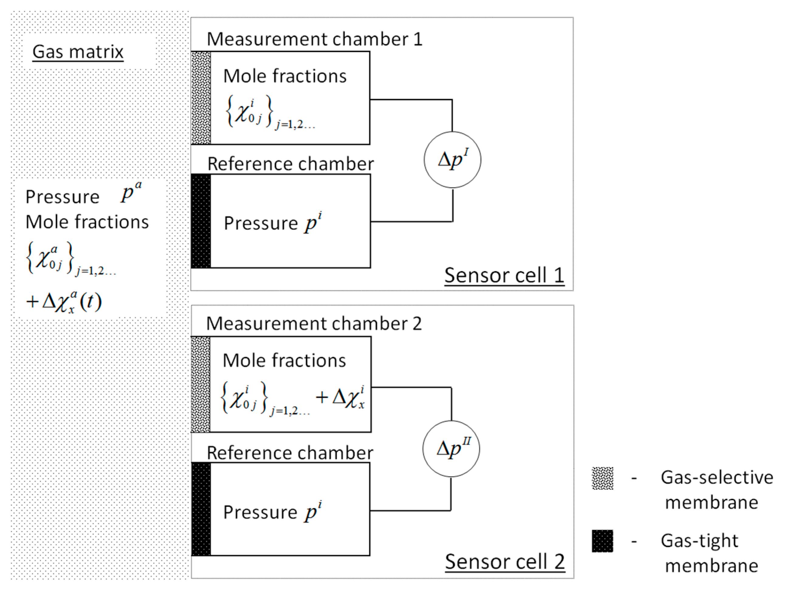
In contrast to that single sensor response, the dynamic behavior of the reference-based sensor response is, according to Equation (5), independent of , which is only included in the offset constant in Equation (3). The ratio compensates for this combined line-sensor response for differences between the initial outer and inner gas compositions. Hence, under given measurement conditions, one expects similar responses for sensors of different geometry, i.e., for planar- or tubular-designed sensor cells, different lengths of line-sensor or different membrane thicknesses. Moreover, the dynamic range of such a sensor must be independent of the target gas component. Therefore, an internal standard-based gas sensor that is adjusted for a gas component, e.g., for CO2, should answer with the same slope (with permeability/selectivity-dependent physical resolution) to another target gas, e.g., argon, chlorine, or hydrogen, as long as the membrane shows permeability differences for this target gas with respect to the initially present gas components. Finally, the application and combination of different membrane materials will be possible, which are best adapted to the target gas component(s) and environmental properties, without changing the internal standard-based (and therefore normalized) response behavior.
Based on the performed experiments, the next sections consider and prove this normalized response behavior for the measurement of the target gas CO2 in air.
4.3. Offset Determination
An offset adjustment is needed to determine the zero-point of the measurement system under the current set of measurement conditions. To adjust the offset constant
in Equation (5), a baseline can be experimentally determined from a time record of
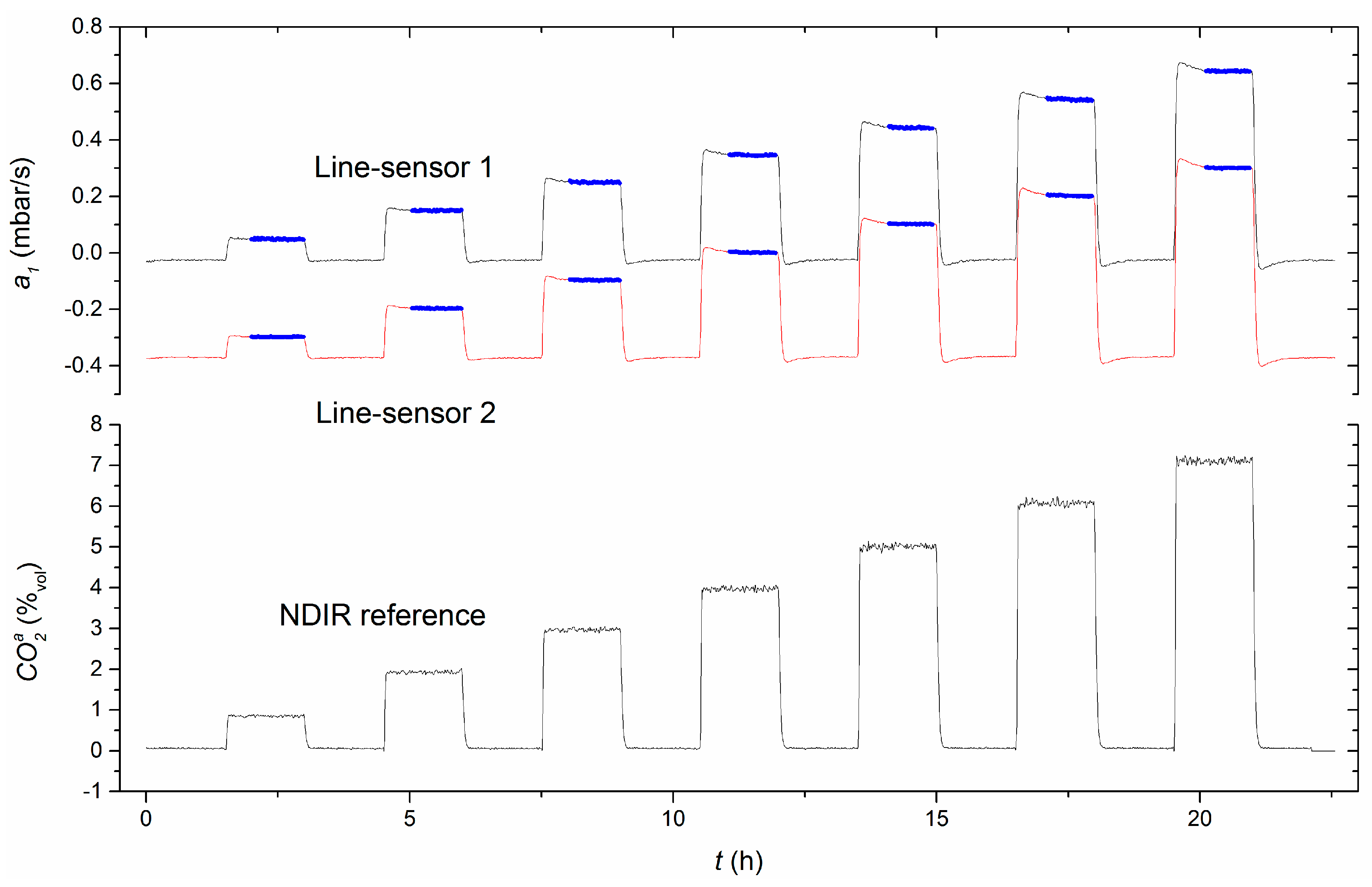
for equivalent gas compositions at both faces of the membrane (e.g., from the measurement values between 0–1.3 h in
Figure 3). Therefore, baseline records of 1 h with about 100 measurement values were analyzed before each experiment. The experimentally determined offsets range between
mbar/s with a mean of
mbar/s.
However, the offset
can also be calculated independently of any experiment according to Equation (7) for the respective measurement conditions, i.e., the gas pressures within and outside the line-sensors, and the initial purge gas composition. The initial purge gas composition {CO
2, Ar + O
2, N
2} was assumed to be
%
vol. Due to its similar permeation coefficients [
33], the contents of argon and oxygen were combined. With respect to the permeability estimates and geometrical measures from
Section 3.1, and the mean purge gas overpressure of 5.5 mbar, the offset results in
mbar/s. Using the permeabilities
cm
3cm/cm
2/s/cmHg from [
34] estimated at 35 °C, the offset results in
mbar/s for same conditions (the unit of permeability that considers the experimental conditions, i.e., the applied pressure in “cmHg”, was converted by 7598 mm
2/s = 1 cm
3cm/cm
2/s/cmHg).
With respect to the approach of a self-calibrating measurement system, only the calculated offset ( mbar/s) with permeabilities from this literature, which fits well with the experimentally determined offsets, will be subsequently considered.
4.4. Temperature Dependency
The permeation process of a gas through a polymeric membrane depends exponentially on temperature: the so-called Arrhenius law. Already in 1939, this strong temperature dependency was considered for rubber-like polymeric membranes in [
35]. The influence of this dependency on the measurement signal of a membrane-based gas sensor was investigated for an experimental temperature range of 297–302 K in [
31]. However, negligible dependency was found within that 5 K range. This unexpected result was attributed to the measurement principle, in which the purge gas partly compensates for the temperature dependency.
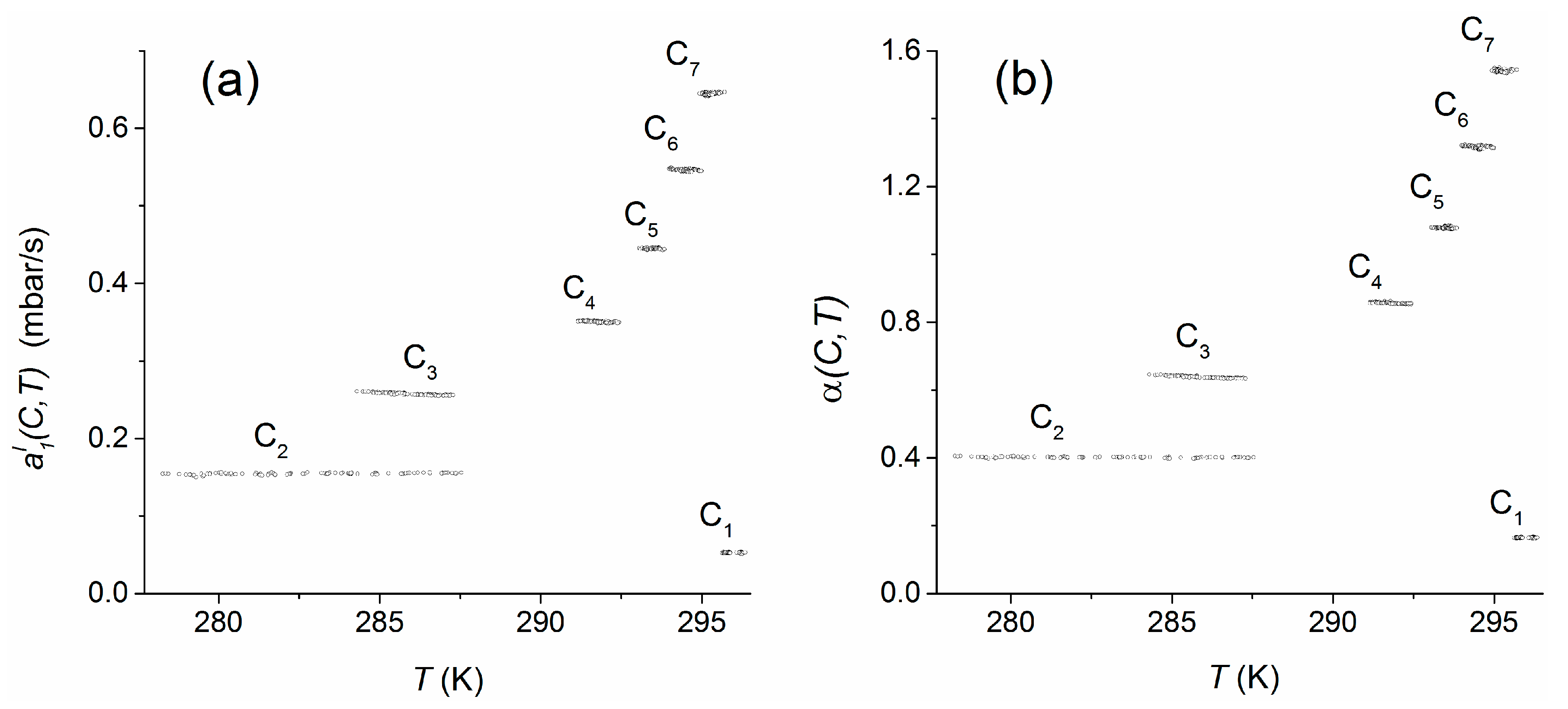
Using the data of experiment 4, the temperature dependency was analyzed for an extended range of about 18 K within 278–296 K for the concentration range C
1–C
7 (see
Appendix A, Table A1) in the test column. The pressure changes
using the calculated offset (
Section 4.3) and
comparable to our previous investigations are shown in
Figure 4.
Compared to the concentration dependence of the measurement signal, both measures seem to be almost constant within the individual concentration plateaus, i.e., they are not significantly influenced by the temperature. For quantification of the temperature dependencies over the whole temperature range, the regression coefficients and , which were obtained by linear regressions of the sensor responses within the individual plateau concentrations (C1–C7), were weighted with respect to the relative numbers of the plateau-measurement values used. To consider the different widths of temperature ranges that were observes within the individual concentration plateaus, each regression coefficient was, in addition, weighted with the relative temperature range covered by the respective plateau. Finally, the weighted regression coefficients were averaged. As a result, the mean temperature dependencies including standard errors were found to be mbar/K and K−1. In both cases, the estimated temperature trends do not significantly influence the measures within the applied temperature range.
4.5. Scaling Behavior of Combined Line-Sensor Response
Whereas the outer transformation behavior of a combined line-sensor response is defined according to Equation (3) by the ratio , the ratio in Equation (4) defines the inner transformation behavior of its response. The reciprocal values and are the outer and inner sensitivity, respectively, of the combined line-sensor.
According to
Section 2 the outer transformation behavior can be calculated in dependence on the measurement conditions for known inner slope. In the present case one held
. However, with respect to the comparison of both signals in Equation (5), the final response behavior of the combined line-sensor signal enables no insight in the internal scaling behavior.
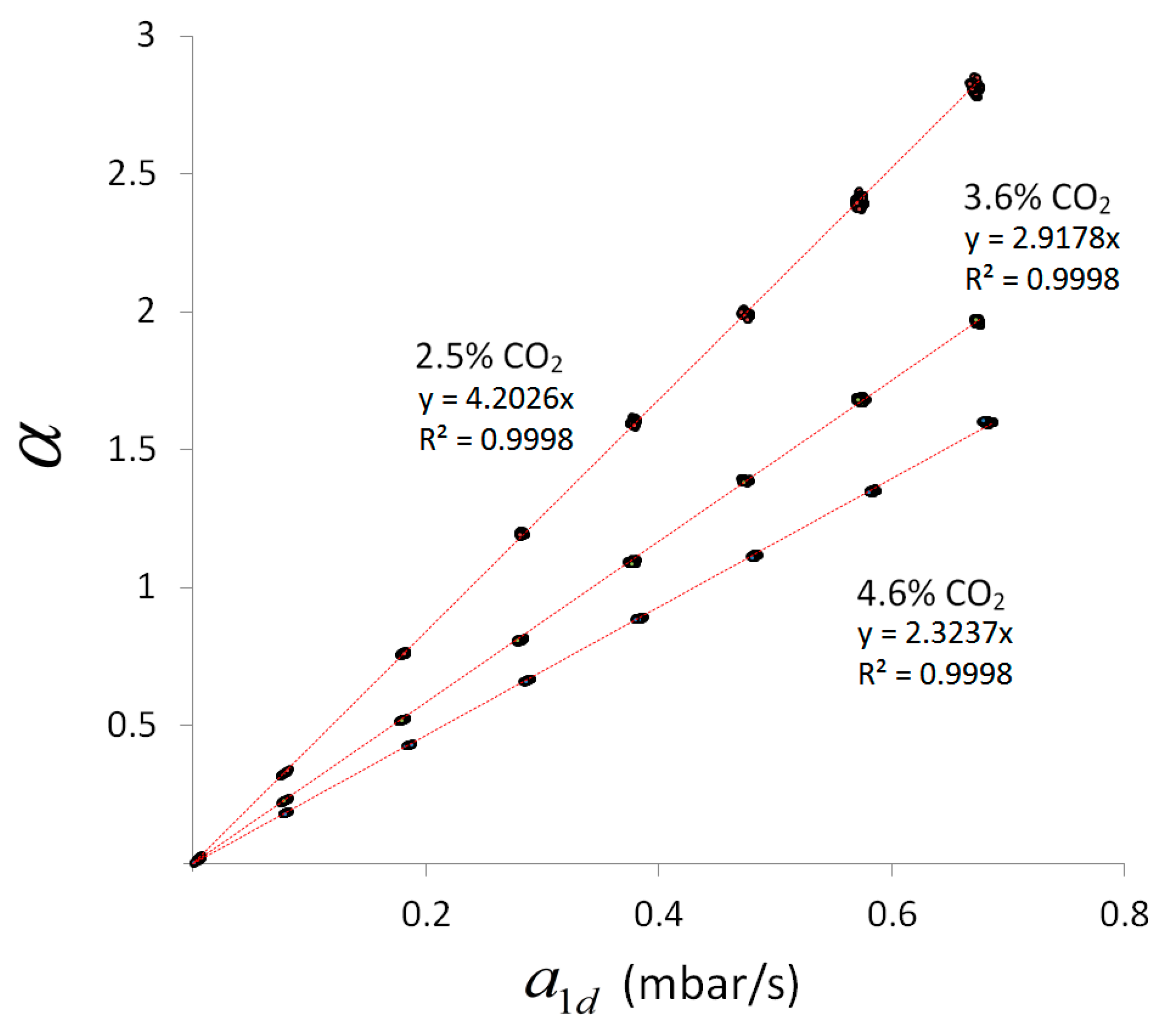
To consider this scaling behavior,
Figure 5 shows a comparison of the pure measurement signals: the combined line-sensor response
for experiments 1–3 with respect to
. The internal standard concentrations used (
Table 3) are indicated in
Figure 5 near the respective dataset. The measurement values (dots) along a regression line (red) represent the behavior of the combined line-sensor response for a particular internal standard concentration and diverse outer CO
2 concentration of up to 7%
vol. Due to the offset subtraction in
and
, the regression lines have to start near the point of origin.
The regression coefficients
of the regression lines in
Figure 5 increase with decreasing concentration of the internal standard
(
Table 3). This behavior results in inner slopes that are given in
Table 3 for the experiments 1–3, and which characterizes the (inner) signal dynamics of the combined line-sensor.
The inner slope can also be calculated according to Equation (4) with respect to the measurement conditions: gas pressures and initial inner gas composition. For given permeabilities and geometrical measures, this theoretical inner slope is 0.033 s/mbar. The most sensitive parameter in Equation (4) that determines this underestimate is the CO
2 permeability that occurs within time constant
. On the other hand, this permeability is the only parameter that does not change the offset according to Equation (7), behaving comparably to the experimental values (
Section 4.3). For a long time [
36], the determination of such permeability values has been performed in single gas experiments based on standardized methods, e.g., applying different gas pressures in the range of several bar to both faces of a membrane, analyzing the steady-state gas flow [
34] and extrapolating the results to a zero-pressure difference. These material parameters can differ from those for mixed gas systems with comparatively small (partial) pressure differences. A fit based on the experimentally determined mean inner slope
s/mbar results in a 2.5-fold smaller effective CO
2 permeability of
m
2/s, and a reduced effective selectivity of
with respect to N
2. Such a reduced selectivity has already been observed in previous mixed gas tests, and has been discussed, e.g., in [
30]. In addition, the decrease in selectivity can be partly attributed to the non-zero permeabilities of the C-Flex-reference membranes [
27].
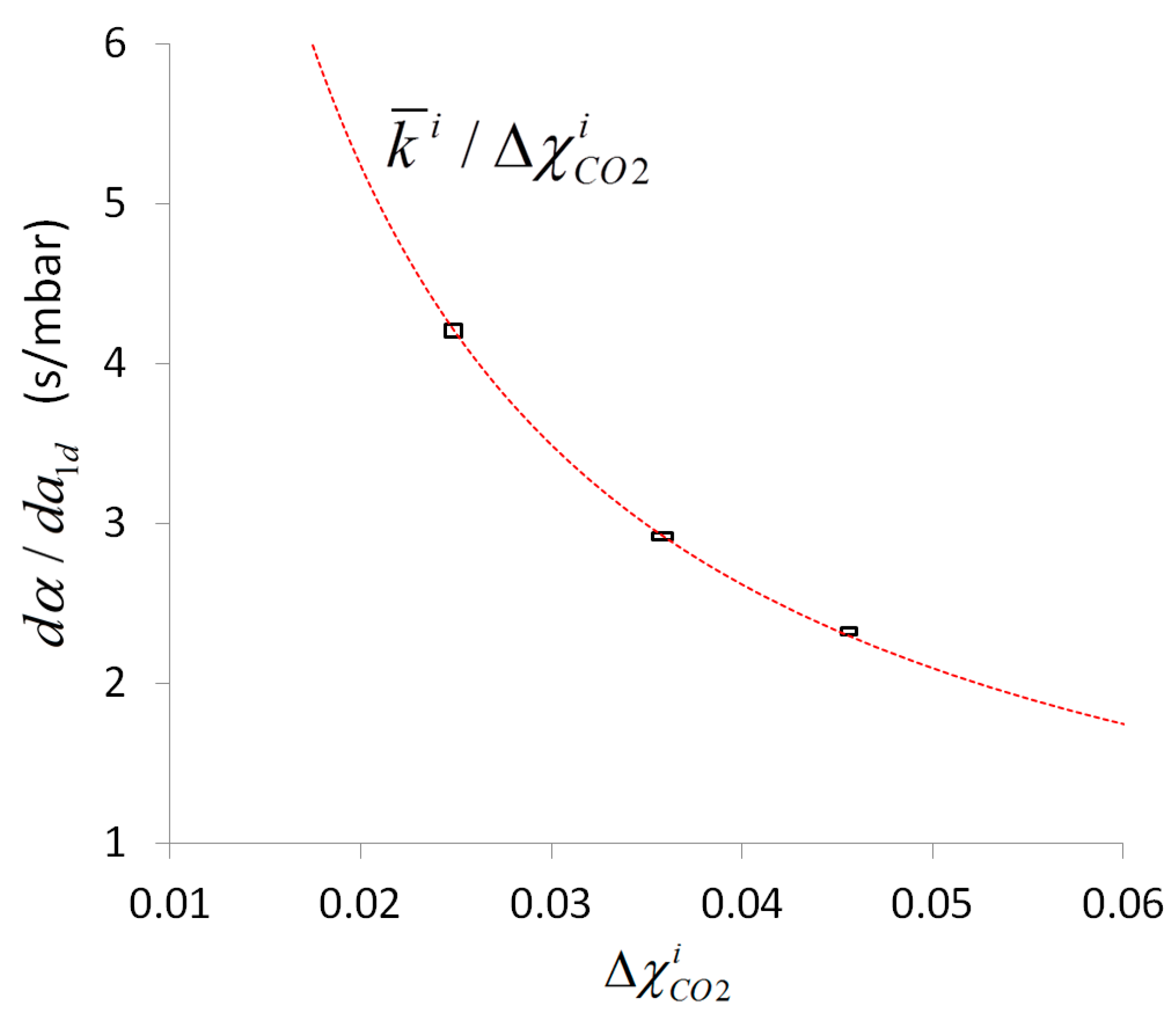
Figure 6 shows the determined individual (real) regression coefficients
from
Table 3 compared to the averaged (ideal) response behavior
(red line). The deviation of the inner slopes
in
Table 3 from the mean inner slope is small. For better visibility, the three-fold standard deviations are shown as rectangles around the experimental means for
and
. These rectangles match the calculated characteristics, i.e., the sensor signal is highly determined by the ratio
and therefore, the inner slope can be considered to a good approximation as independent of the internal standard concentration. Moreover,
Figure 6 shows that the same variation of internal standard concentration results for smaller
in an increased error propagation into the sensor response. Taking both aspects into account,
is a key parameter that can be calculated based on material parameters and used to configure an application specific optimal design of the combined line-sensor with defined sensitivity (in the present case the inner sensitivity is
mbar/s and the outer is
mbar/s). Moreover, based on the measurement values, this parameter can be recorded, e.g., in terms of a technical production specification, and it enables the sensor to check for its functional reliability during running applications, or to check a change of sensitivity, due to outer pollution, aging and fouling of the membrane.
According to
Table 4 that shows the regression results between the primary line-sensor signals
and
, the experiments demonstrate a highly correlated response behavior of both line-sensors with Pearson’s squared correlation coefficients at
. The line-sensors show nearly the same slopes (regression coefficient
in
Table 4) with deviations smaller than 1%. The distance of the response of line-sensors 1 and 2 (intercept
in
Table 4) increases with increasing concentration of the internal standard. If
, which according to
Table 4 is a good approximation, then the difference
will be independent of the outer concentration, which can be considered as an ideal scaling behavior. This difference can be calculated based on the intercept
, i.e., for a discrete point near
. A comparison of
with
from the investigated complete concentration range shows a deviation smaller than 0.4%. Thus, also a simple regression of the primary line-sensor responses can be used to estimate the inner slope with
. In addition, such a regression can be performed during a running application.
4.6. Impact of Fluctuations of Internal Standard Concentration
Section 4.1,
Section 4.2,
Section 4.3,
Section 4.4 and
Section 4.5 have essentially considered the behavior of the combined line-sensor. However, as shown in
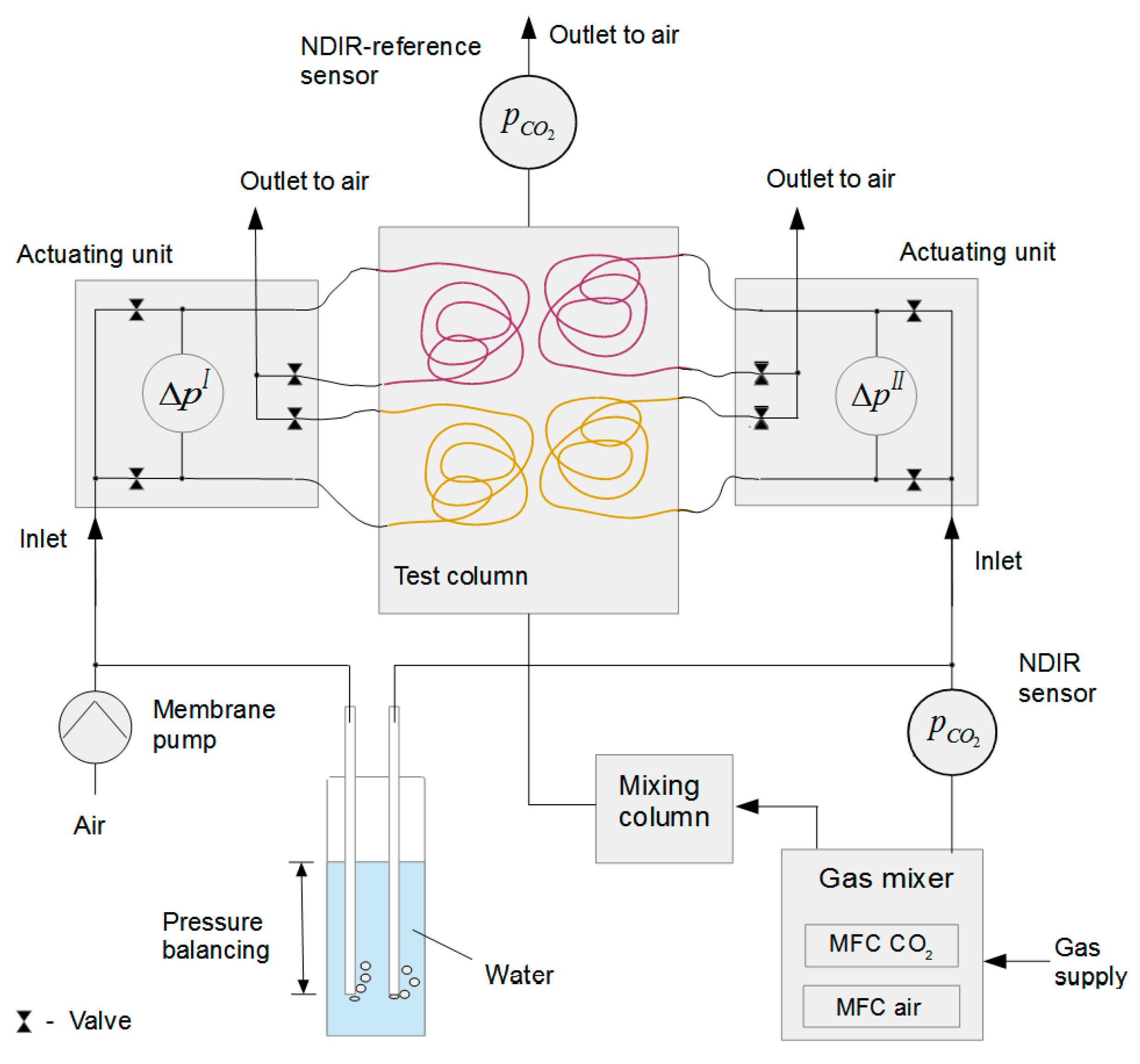
Figure 6, fluctuation of the internal standard concentration influences the dispersion of its response. Such fluctuations, produced during the mixing process by the MFCs, will be recorded as slightly smoothed by the NDIR reference sensor that was situated in the purge gas line between the MFCs and line-sensor 2 (
Figure 2). They will be further smoothed on the way to the line-sensor and, in addition, as a result of the comparatively slow diffusion process through the sensor membrane. If so, a smoothing of the NDIR reference sensor signal should result in a more appropriate internal standard signal.
The highest fluctuations of
(
Figure 6) were observed in experiment 2. Therefore, the impact of such a smoothing will be considered for this experiment. Taking into account that only older
readings contribute to a combined line-sensor response at a time
, unidirectional moving averages
were applied over different numbers of readings from
(i.e., no smoothed original data) to 10 to smooth the internal standard concentration at
.
Using the smoothed records of internal standard concentration the respective responses of the combined line-sensor were recalculated according to Equations (5) and (6) for the various concentration plateaus, and mean standard deviations were determined based on the concentration-weighted standard deviations of this plateau concentrations.
Figure 7 shows the influence of smoothing resulting in a decrease of fluctuations of the internal standard concentration (standard deviation
) for increasing size
of the moving average. At the same time, the mean standard deviation
decreases asymptotically. For a size
of moving average, the outer dispersion
%
vol of the combined line-sensor response has the same order of magnitude as the equivalent weighted mean dispersion
%
vol achieved by the NDIR reference sensor. Linear extrapolation of this smoothing behavior to a (mathematical) constant internal standard concentration results in an expectation value for the asymptotic mean outer dispersion of
%
vol for the combined line-sensor response. Thus, the most accurate measurement values could be expected for using, e.g., a (certified) gas mixture from a simple gas container.
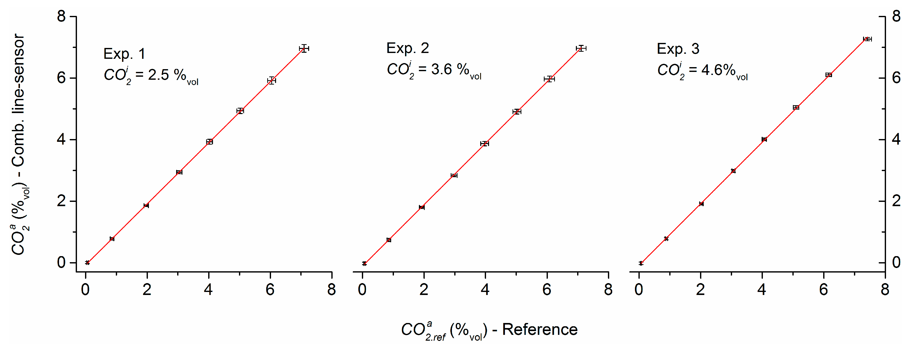
4.7. Measurement Comparison of Combined Line-Sensor and NDIR Reference
Figure 8 shows as black error bars the result of measurement comparison analyzed with the combined line-sensor
and the NDIR reference
in the test column for experiments 1–3. These combined line-sensor responses were not calibrated. The smoothing interval of the internal standard concentration was set to
. To obtain the dynamic pressure change
according to Equation (5), the offset
mbar/s (calculated in
Section 4.3) was uniformly reduced from
in all data records. Linear regressions
with the NDIR reference concentration
(
—regression coefficient and intercept,
,
—respective standard errors) demonstrate the linear behavior of sensor response. The strong similarity of both sensor responses is also documented by the fit constants in
Table 5.
For comparison, using the experimentally determined individual offsets
(
Section 4.3) instead of the calculated offset
in regressions
does not change the regression coefficients
. It only slightly reduces the distances of the intercepts
of regression (
Table 6) with respect to the expectation (
%
vol).
The high-level consistency of the sensor responses during the measurement comparison was not a priori expected. Differences are possible in the permeabilities of the PDMS tubes with respect to the PDMS material that was used in [
34] for permeability characterization, and the values of permeability can be dependent on the characterization method. In addition, the permeabilities of the C-Flex reference membranes were not considered in this study, tolerances can occur of geometrical measures, and setup-based limitations exist for the exact estimation, e.g., of purge gas pressure. Therefore, further investigations are necessary to obtain a consistent picture about the accuracy of the calibration-free approach, especially, in terms of a reduction of uncertainties in the membrane parameters.


