
Use of Distributed Temperature Sensing Technology to Characterize Fire Behavior


Abstract
:1. Introduction
2. Experimental Section
2.1. Study Site
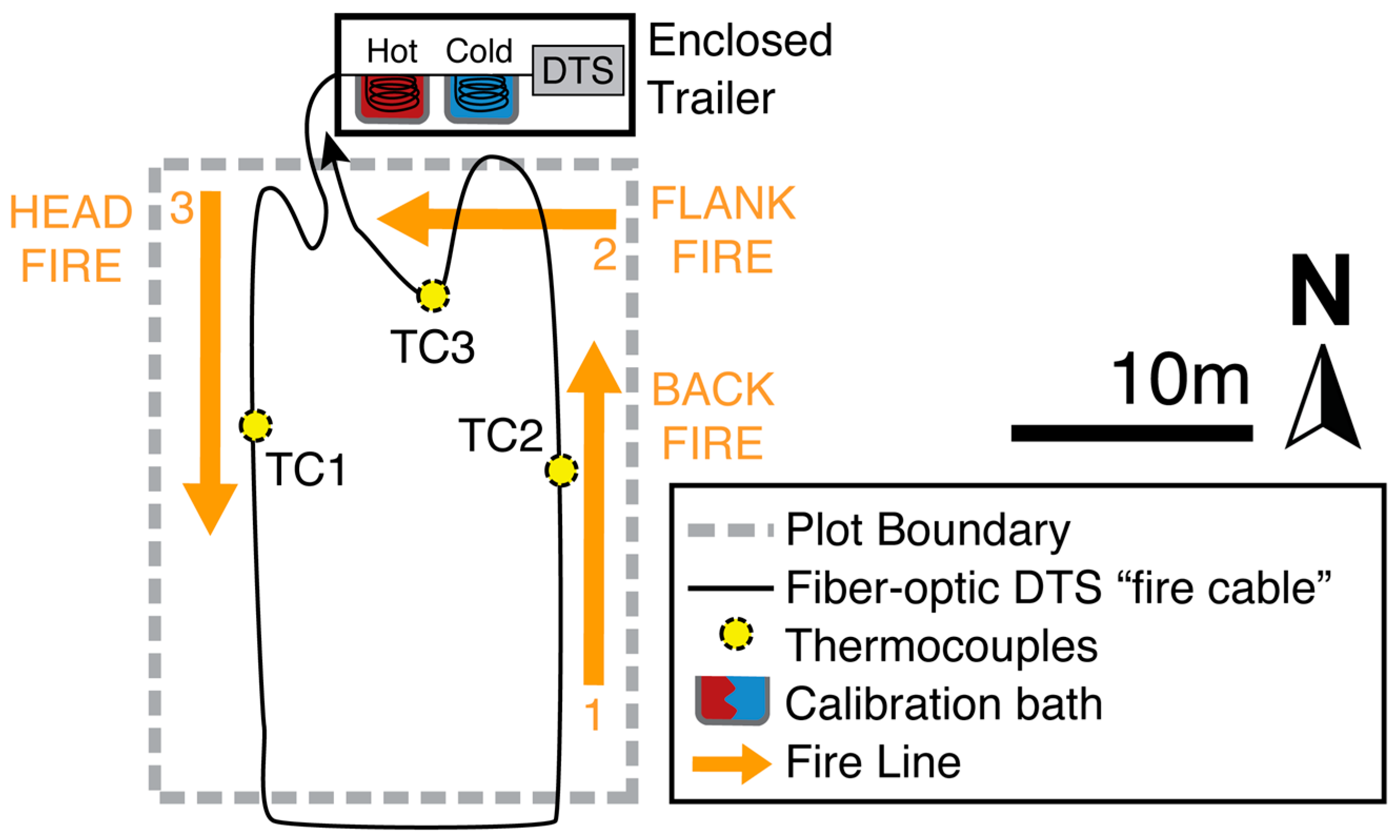
2.2. Study Design
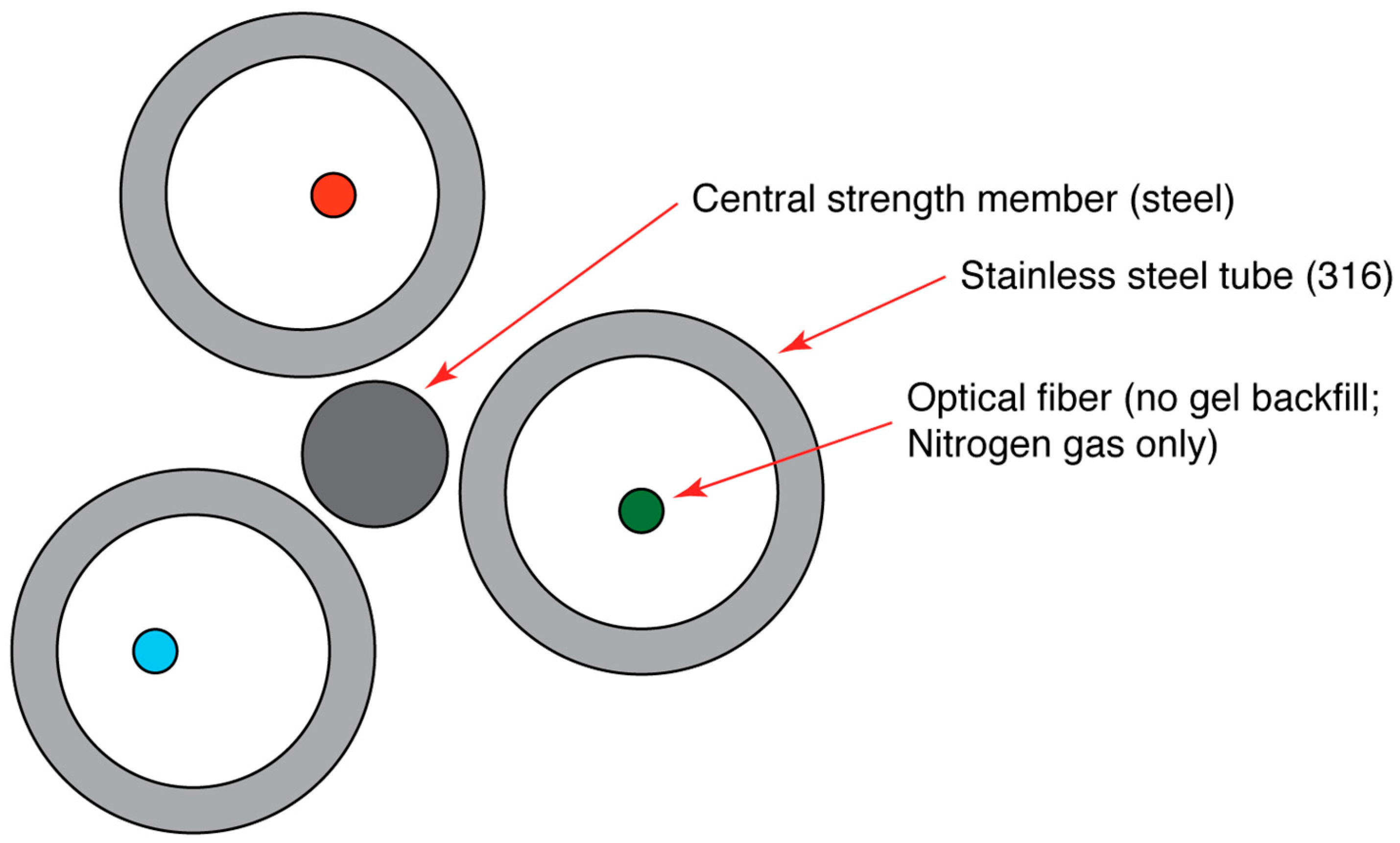
2.3. DTS Technology
2.4. Field Data Collection
3. Results and Discussion
4. Conclusions
Supplementary Materials
Acknowledgments
Author Contributions
Conflicts of Interest
References
- Finney, M.A. Calculation of fire spread rates across random landscapes. J. Int. Assoc. Wildland Fire 2003, 12, 167–174. [Google Scholar] [CrossRef]
- Kremens, R.L.; Smith, A.M.S.; Dickinson, M.B. Fire metrology: Current and future directions in physics-based methods. Fire Ecol. 2010, 6, 13–35. [Google Scholar] [CrossRef]
- Iverson, L.R.; Yaussy, D.A.; Rebbeck, J.; Hutchinson, T.F.; Long, R.P.; Prasad, A.M. A comparison of thermocouples and temperature paints to monitor spatial and temporal characteristics of landscape-scale prescribed fires. J. Int. Assoc. Wildland Fire 2004, 13, 311–322. [Google Scholar] [CrossRef]
- Bova, A.S.; Dickinson, M.B. Beyond “fire temperatures”: Calibrating thermocouple probes and modeling their response to surface fires in hardwood fuels. Can. J. For. Res. 2008, 38, 1008–1020. [Google Scholar] [CrossRef]
- Selker, J.S.; Thévenaz, L.; Huwald, H.; Mallet, A.; Luxemburg, W.; Van de Geisen, N.; Stejskal, M.; Zeman, J.; Westoff, M.; Parlange, M.B. Distributed fiber-optic temperature sensing for hydrologic systems. Water Resour. Res. 2006, 42, 1–8. [Google Scholar] [CrossRef]
- Thomas, C.K.; Kennedy, A.M.; Selker, J.S.; Moretti, A.; Schroth, M.H.; Smoot, A.R.; Tufillaro, N.B.; Zeeman, M.J. High-resolution fibre-optic temperature sensing: A new tool to study the two-dimensional structure of atmospheric surface layer flow. Boundary Layer Meteorol. 2012, 142, 177–192. [Google Scholar] [CrossRef]
- Tyler, S.W.; Holland, D.M.; Zagorodnov, V.; Stern, A.A.; Sladek, C.; Kobs, S.; White, S.; Suárez, F.; Bryenton, J. Using distributed temperature sensors to monitor an Antarctic ice shelf and sub-ice-shelf cavity. J. Glaciol. 2013, 59, 583–591. [Google Scholar] [CrossRef]
- Sun, M.; Tang, Y.; Yang, S.; Li, J.; Sigrist, M.W.; Dong, F. Fire source localization based on distributed temperature sensing by a dual-line optical fiber system. Sensors 2016, 16, 829. [Google Scholar] [CrossRef] [PubMed]
- Liu, Z.; Kim, A.K. Review of recent developments in fire detection technologies. J. Fire Prot. Eng. 2003, 13, 129–151. [Google Scholar] [CrossRef]
- Noguchi, K.; Shibata, N.; Uesugi, N.; Negishi, Y. Loss increase for optical fibers exposed to hydrogen atmosphere. J. Lightwave Technol. 1985, 3, 236–243. [Google Scholar] [CrossRef]
- Lemaire, P.J. Reliability of optical fibers exposed to hydrogen: Prediction of long-term loss increases. Opt. Eng. 1991, 30, 780–789. [Google Scholar] [CrossRef]
- Reinsch, T.; Henninges, J. Temperature-dependent characterization of optical fibres for distributed temperature sensing in hot geothermal wells. Meas. Sci. Technol. 2010, 21, 094022. [Google Scholar] [CrossRef]
- Torell, L.A.; McDaniel, K.C.; Cox, S.; Majumdar, S. Eighteen Years (1990–2007) of Climatological Data on NMSU’s Corona Range and Livestock Research Center. Available online: Http://aces.nmsu.edu/pubs/research/weather_climate/RR761/welcome.html (accessed on 10 October 2016).
- McDaniel, K.; Hart, C.; Carroll, D. Broom snakeweed control with fire on New Mexico blue grama rangeland. J. Range Manag. 1997, 50, 652–659. [Google Scholar] [CrossRef]
- Tyler, S.W.; Selker, J.S.; Hausner, M.B.; Hatch, C.E.; Torgersen, T.; Schladow, G. Environmental Temperature Sensing Using Raman Spectra DTS Fiber-Optic Methods. Water Resour. Res. 2009, 4, 673–679. [Google Scholar] [CrossRef]
- Kennard, D.K.; Outcalt, K.W.; Jones, D.; O’Brien, J.J. Comparing techniques for estimating flame temperature of prescribed fires. Fire Ecol. 2005, 1, 75–84. [Google Scholar] [CrossRef]
- Neilson, B.T.; Hatch, C.E.; Ban, H.; Tyler, S.W. Effects of solar radiative heating on fiber-optic cables used in aquatic applications. Water Resour. Res. 2010, 46, W08540. [Google Scholar]
- Swezy, D.M.; Agee, J.K. Prescribed-fire effects on fine-root and tree mortality in old-growth ponderosa pine. Can. J. For. Res. 1991, 21, 626–634. [Google Scholar] [CrossRef]
- Drewa, P.B.; Platt, W.J.; Moser, E.B. Fire effects on resprouting of shrubs in headwaters of southeastern longleaf pine savannas. Ecology 2002, 83, 755–767. [Google Scholar] [CrossRef]


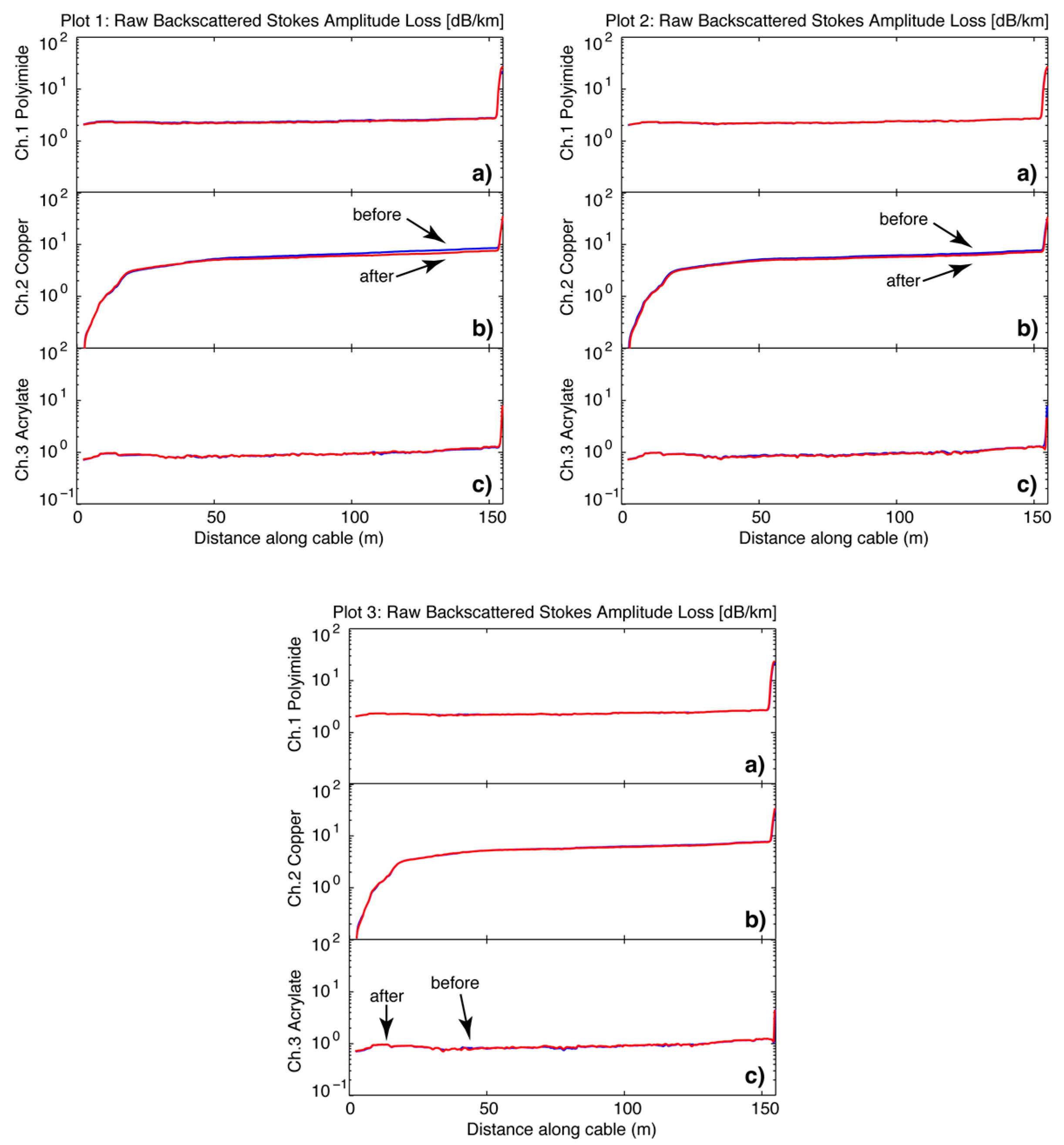
| DTS Fiber Coating | Before Burn | After Burn | Change b,c | |||
|---|---|---|---|---|---|---|
| Loss (dB) | Length (m) a | Attenuation (dB/km) | Loss (dB) | Attenuation (dB/km) | Attenuation (dB/km) | |
| Polyimide | 0.22 | 100.7 | 2.1 | 0.13 | 1.9 | −0.81 |
| Copper | 1.49 | 11.8 | 126.8 | 1.60 | 135.8 | 9.53 |
| 2.63 | 33.0 | 79.7 | 2.19 | 69.3 | −13.35 | |
| 2.96 | 95.8 | 30.9 | 2.11 | 24.5 | −8.78 | |
| Acrylate | 0.26 | 121.2 | 2.2 | 0.28 | 2.3 | 0.12 |
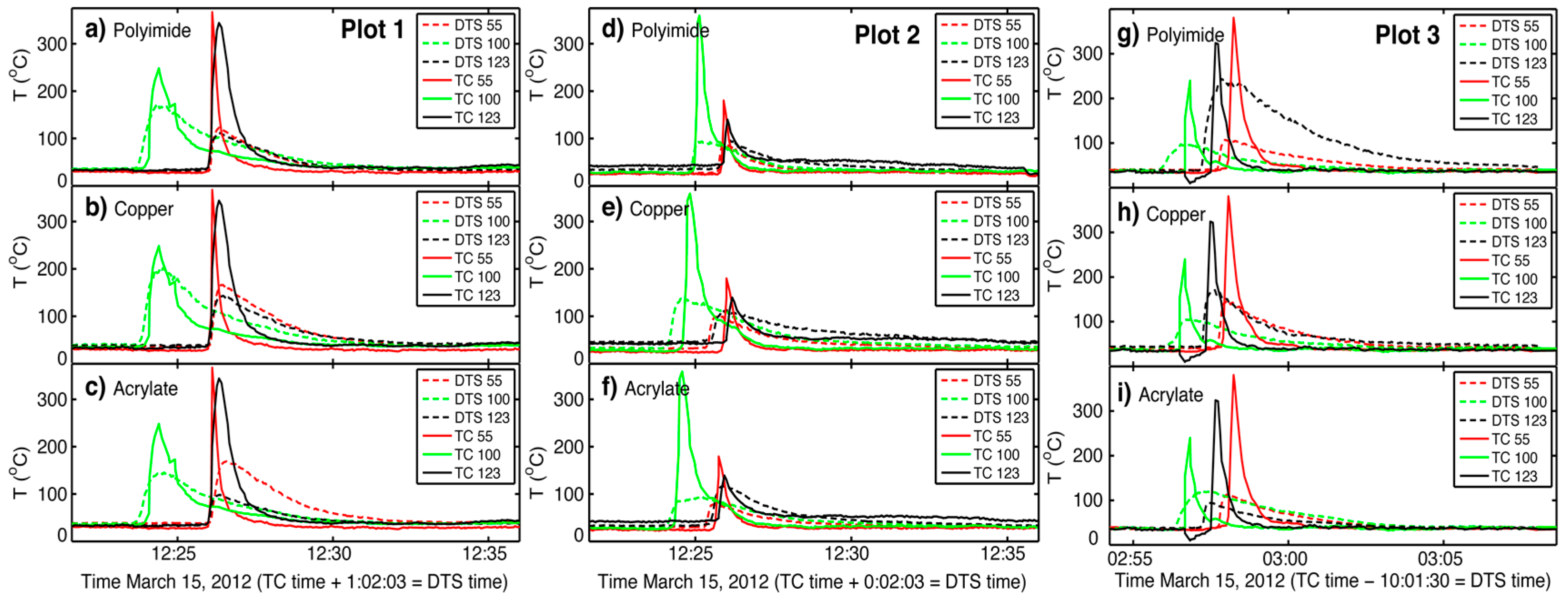
| Location and Sensor | T (°C) at 55 m a | T (°C) at 100 m | T (°C) at 123 m | Absolute Maximum T (°C) b | Location (m) c | |
|---|---|---|---|---|---|---|
| Plot 1 | ||||||
| Thermocouple | 366.7 | 248.1 | 344.0 | |||
| DTS fiber coating | ||||||
| polyimide | 122.7 | 173.1 | 112.3 | 307.1 | 104 | |
| copper | 166.1 | 202.3 | 98.5 | 421.9 | 105 | |
| acrylate | 169.1 | 145.7 | 143.2 | 310.1 | 106 | |
| Plot 2 | ||||||
| Thermocouple | 184.4 | 363.2 | 144.1 | |||
| DTS fiber coating | ||||||
| polyimide | 91.7 | 97.6 | 100.1 | 178.1 | 118 | |
| copper | 105.1 | 141.7 | 132.4 | 223.2 | 118 | |
| acrylate | 82.81 | 100.8 | 122.2 | 178.3 | 119 | |
| Plot 3 | ||||||
| Thermocouple | 380.7 | 239.6 | 324.0 | |||
| DTS fiber coating | ||||||
| polyimide | 108.9 | 97.1 | 243.4 | 243.4 | 123 | |
| copper | 147.9 | 105.4 | 170.6 | 395.2 | 124 | |
| acrylate | 113.6 | 121.4 | 94.0 | 254.2 | 125 | |
| Fire Behavior Parameter | Definition | Fire Cable and DTS Technology | Alternative Methods |
|---|---|---|---|
| Rate of spread (m/min) | The linear rate of advance of a fire front in the direction perpendicular to the fire front | Potential Strengths: precise and continuous quantification of time interval between flaming front passage at two points. Weakness: while the fire cable allows for relatively prodigious spatial estimates compared to thermocouples, there are still spatial limitations as fire burns in three dimensions | Hand-held stop watch method is inexpensive but does not produce precision estimates necessary for physics based models. A series of thermocouples, while generally inexpensive, inherently result in spatial gaps that reduce temporal precision and requires numerous wires. Airborne remote sensing lacks the necessary temporal and spatial precision due to resolution limitations |
| Heat duration (time) | The length of time that heat occurs at a given point. Time at lethal heat (e.g., >60 °C) is often cited | Potential Strengths: given appropriate temperature calibration, greater temporal and spatial quantification as opposed to thermocouples Weakness: similar to thermocouples, temperature calibration is necessary; potential for heat capacity challenges; and cannot easily measure elevated temperatures (e.g., 10 cm above the soil surface) | Thermocouples are frequently used to measure surface heat duration with modest success |
© 2016 by the authors; licensee MDPI, Basel, Switzerland. This article is an open access article distributed under the terms and conditions of the Creative Commons Attribution (CC-BY) license (http://creativecommons.org/licenses/by/4.0/).
Share and Cite
Cram, D.; Hatch, C.E.; Tyler, S.; Ochoa, C. Use of Distributed Temperature Sensing Technology to Characterize Fire Behavior. Sensors 2016, 16, 1712. https://doi.org/10.3390/s16101712
Cram D, Hatch CE, Tyler S, Ochoa C. Use of Distributed Temperature Sensing Technology to Characterize Fire Behavior. Sensors. 2016; 16(10):1712. https://doi.org/10.3390/s16101712
Chicago/Turabian StyleCram, Douglas, Christine E. Hatch, Scott Tyler, and Carlos Ochoa. 2016. "Use of Distributed Temperature Sensing Technology to Characterize Fire Behavior" Sensors 16, no. 10: 1712. https://doi.org/10.3390/s16101712
APA StyleCram, D., Hatch, C. E., Tyler, S., & Ochoa, C. (2016). Use of Distributed Temperature Sensing Technology to Characterize Fire Behavior. Sensors, 16(10), 1712. https://doi.org/10.3390/s16101712