
Measurement and Evaluation of the Gas Density and Viscosity of Pure Gases and Mixtures Using a Micro-Cantilever Beam


Abstract
:1. Introduction
1.1. Current State of the Art
1.2. Current Approach

2. Methods and Materials
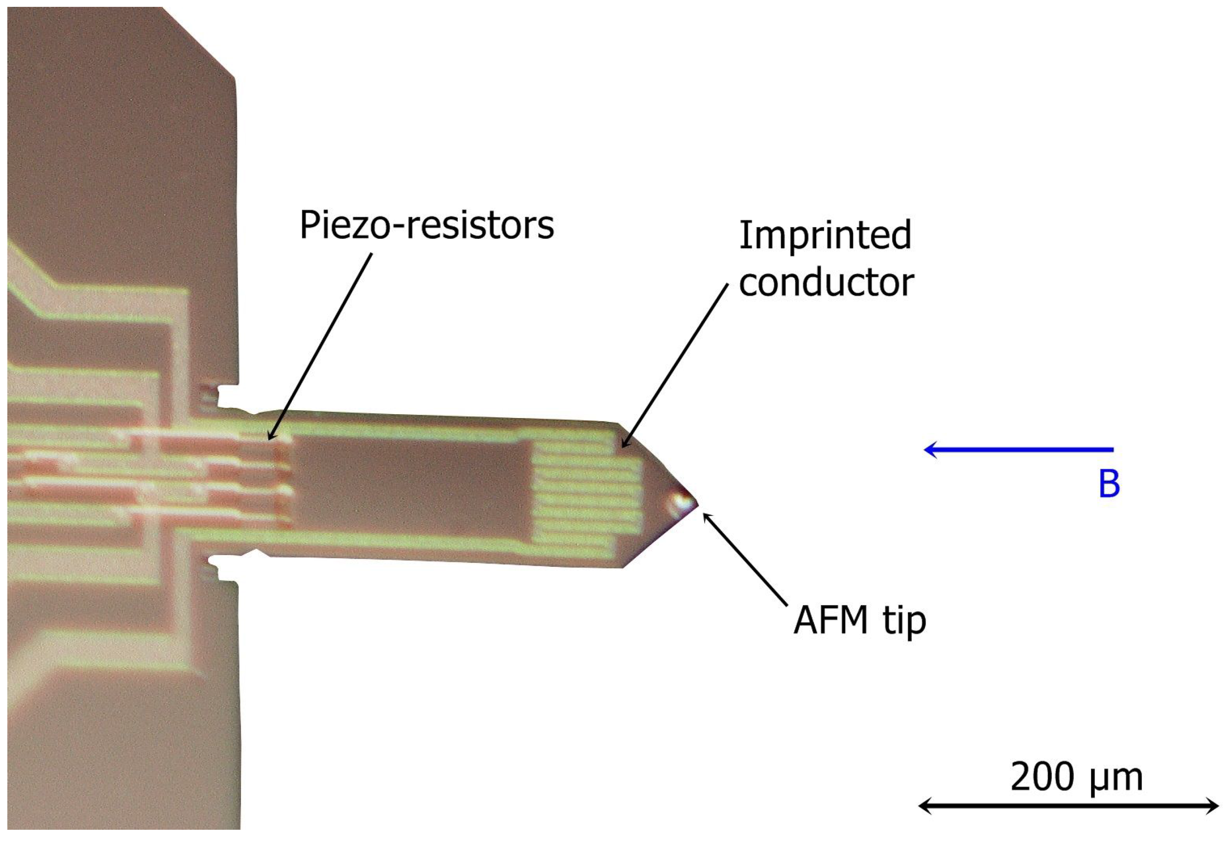
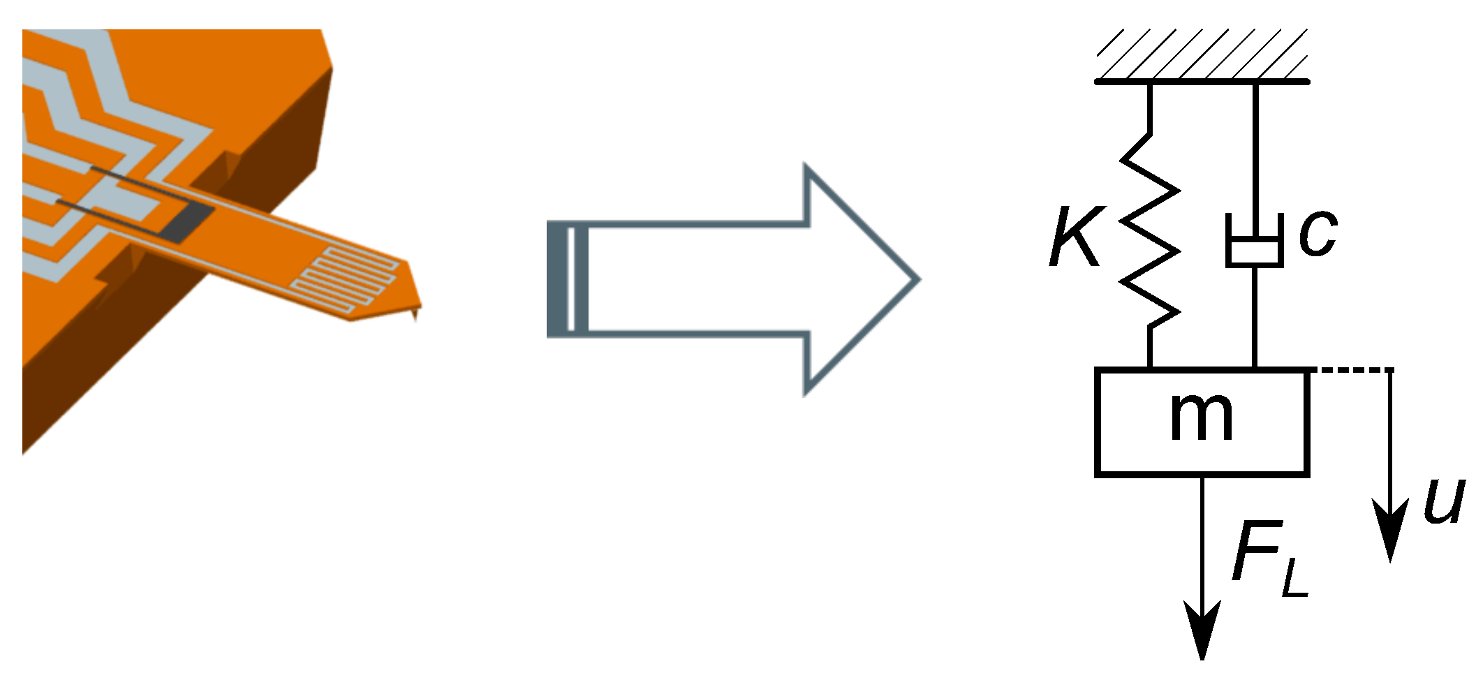
2.1. Sensor
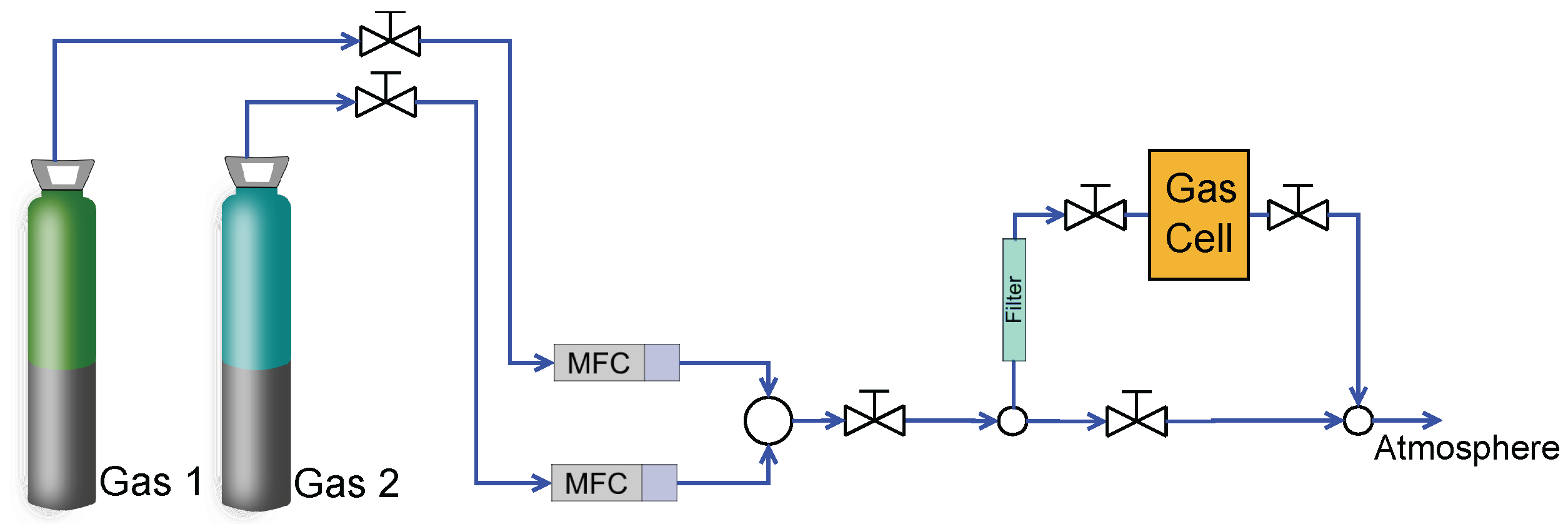
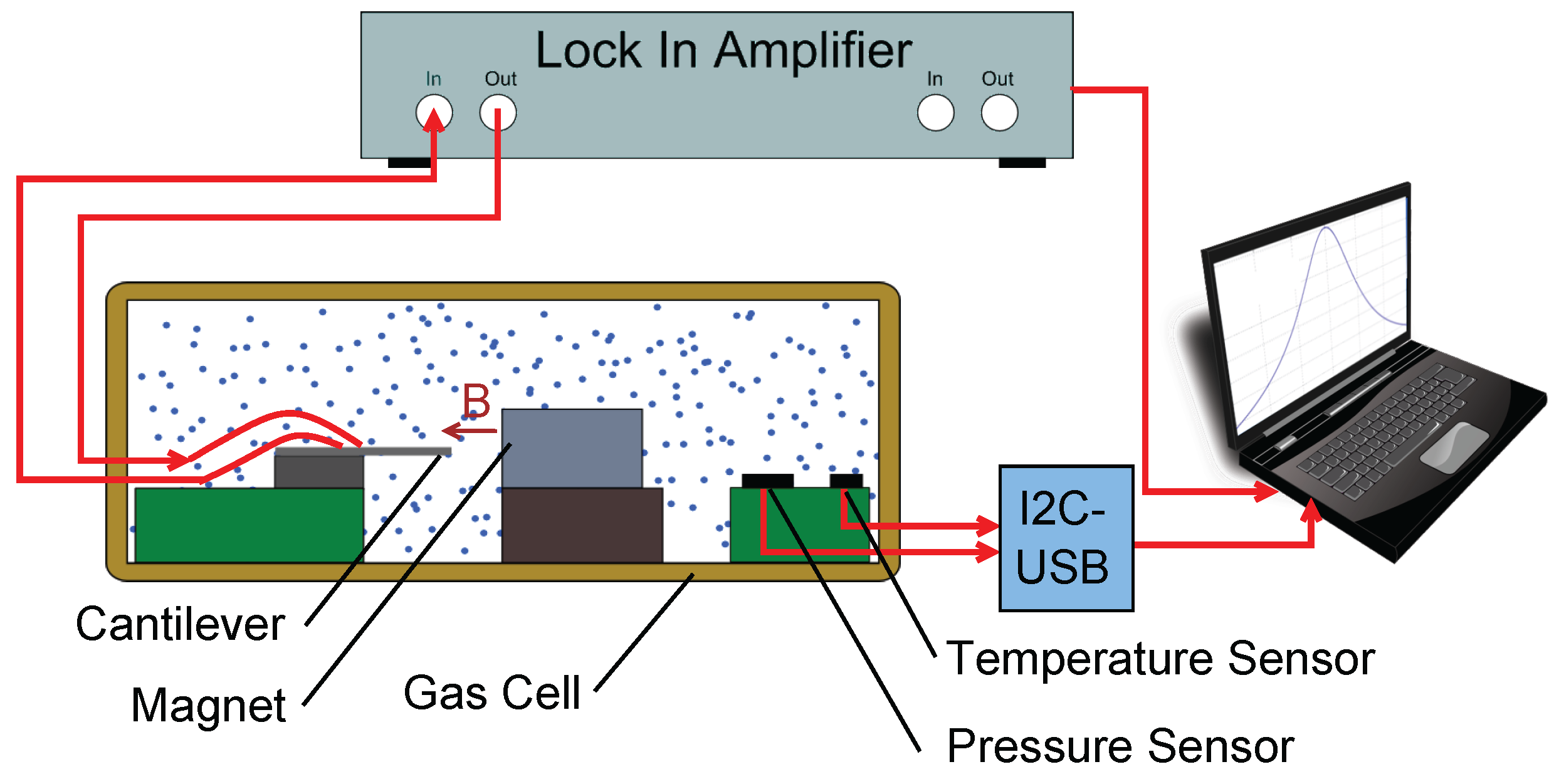
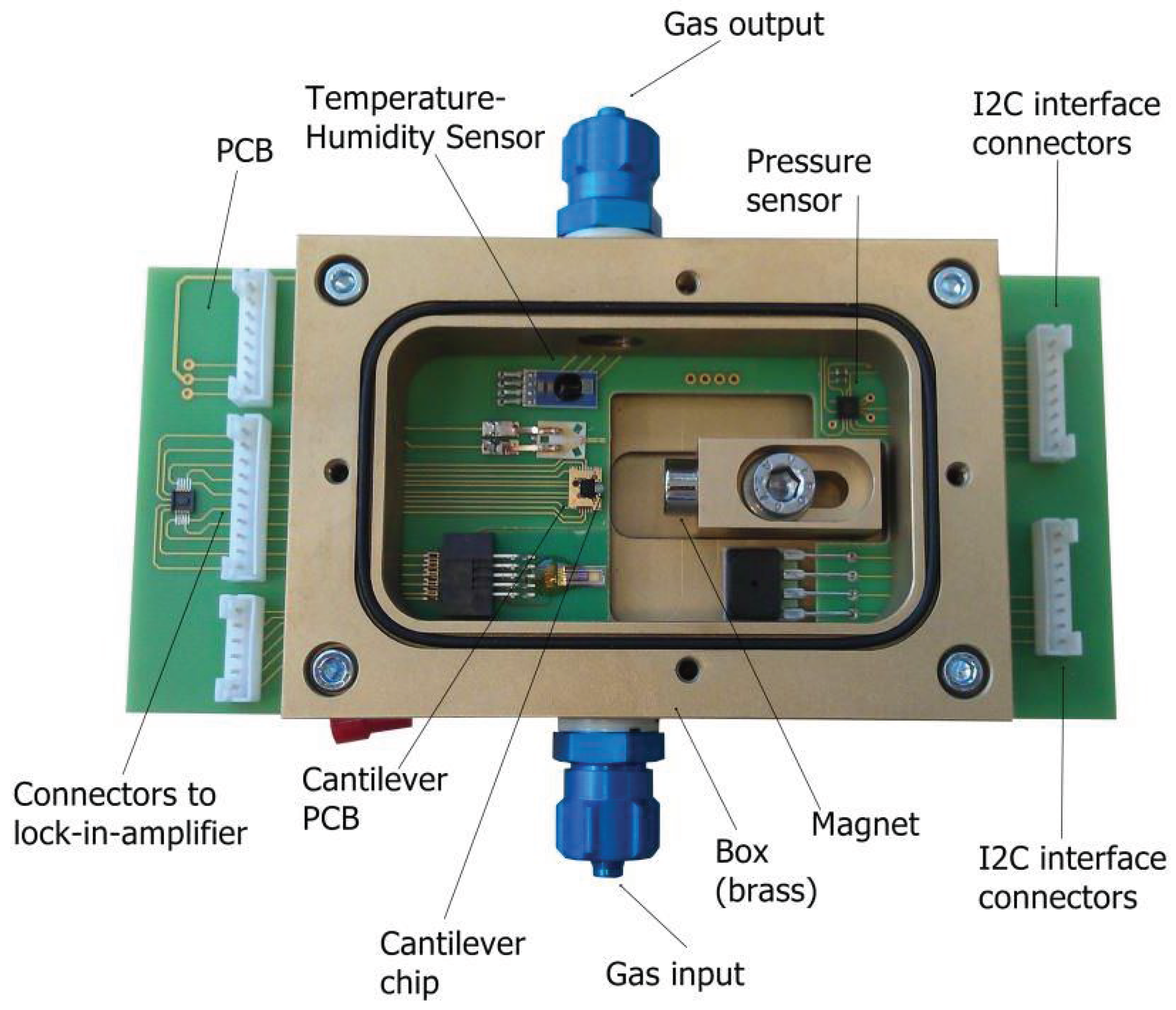
2.2. Experimental Setup

| Gas | (bar) | (K) | (kg/m) | (μPa·s) |
|---|---|---|---|---|
| 0.912 | 297.6 | 1.629 | 14.91 | |
| 0.910 | 297.8 | 1.384 | 17.88 | |
| 0.912 | 298.0 | 1.200 | 20.80 | |
| 0.912 | 298.0 | 1.033 | 24.06 | |
| 0.940 | 297.7 | 0.766 | 31.69 | |
| 0.910 | 297.5 | 0.147 | 19.86 | |
| 0.915 | 296.9 | 1.039 | 17.82 | |
| 0.913 | 297.7 | 0.886 | 17.83 | |
| 0.914 | 297.9 | 1.475 | 22.75 | |
| 0.912 | 298.2 | 1.047 | 23.47 | |
| 0.913 | 297.8 | 1.033 | 17.14 | |
| 0.910 | 298.1 | 0.569 | 23.60 | |
| 0.954 | 296.8 | 1.392 | 22.94 | |
| 0.912 | 297.8 | 1.003 | 17.28 | |
| 0.910 | 297.7 | 0.359 | 22.70 | |
| 0.916 | 297.6 | 1.186 | 20.51 | |
| 0.953 | 297.7 | 0.923 | 27.62 | |
| 0.913 | 297.7 | 1.486 | 16.58 | |
| 0.911 | 298.2 | 0.807 | 23.72 | |
| 0.943 | 298.0 | 1.357 | 15.99 | |
| 0.913 | 297.9 | 1.260 | 23.12 | |
| 0.914 | 297.3 | 1.065 | 18.36 |

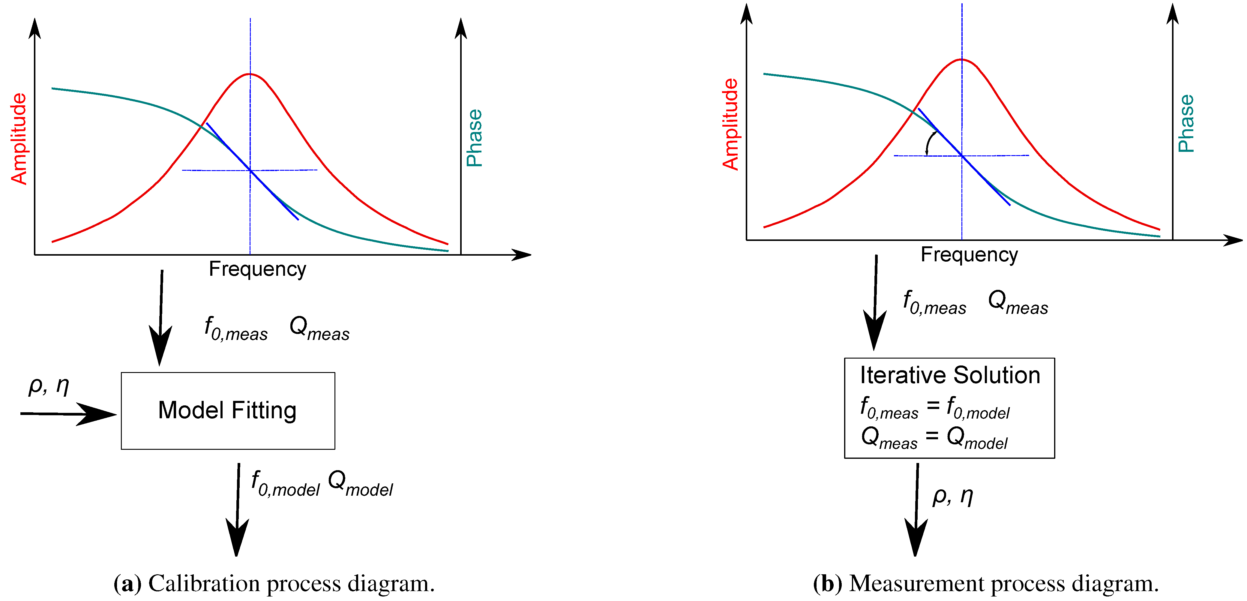
2.3. Modeling
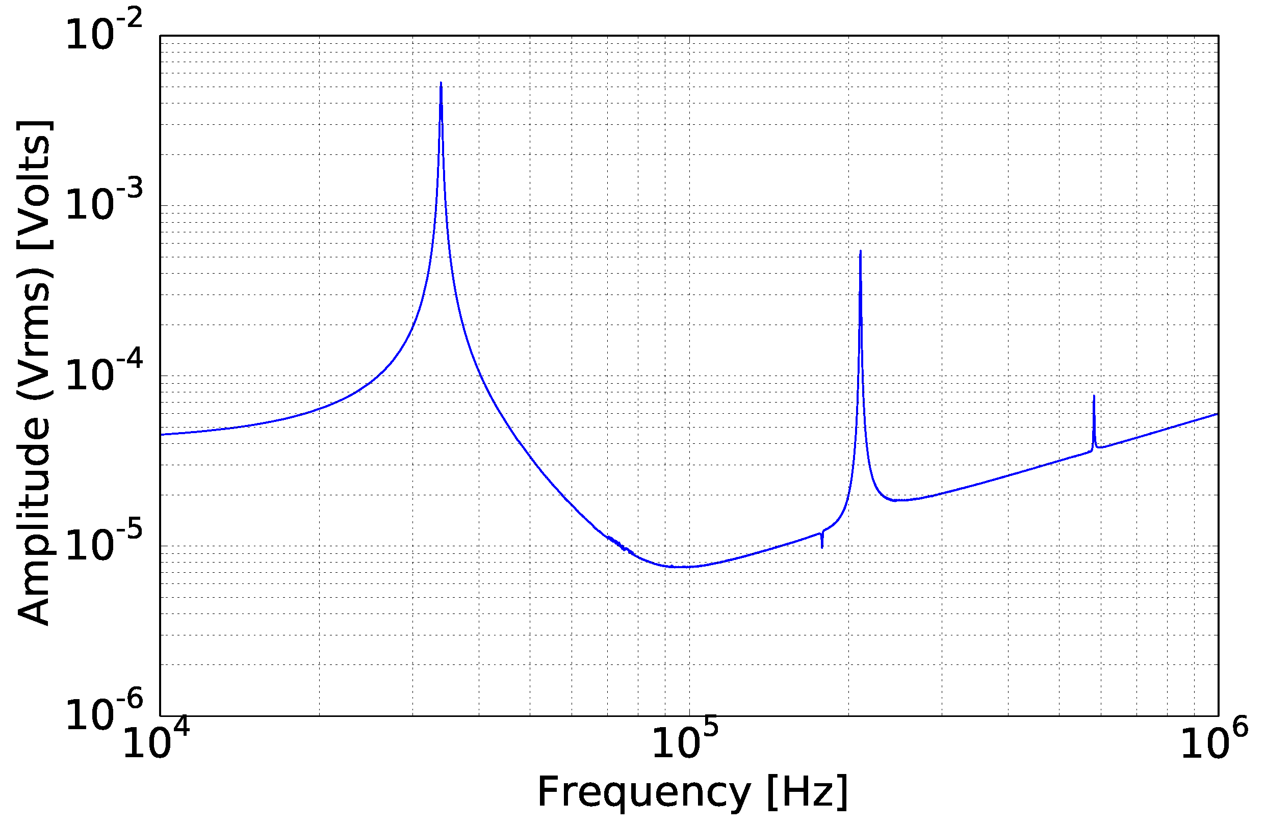
2.4. Quality Factor Measurement
2.5. Calibration Measurement

3. Results Discussion
3.1. Sensor Characterization


| Theory | 6.288 | 17.693 |
| Measurement | 6.204 | 17.138 |
| Deviation | 1.35% | 3.23% |

3.2. Response in Gases


3.3. Performance

3.4. Uncertainty Analysis
| Mixture | Mixtures | Overall | Overall | |||||
|---|---|---|---|---|---|---|---|---|
| (0.2 K) | (20 Pa) | Database | Composition | Mixtures | Pure Gases | |||
| –0.066 | 0.02 | 0.8 | 0.03 | 2 | 1 | 2.376 | 0.8035 | |
| 0.052 | 0.2 | 0.03 | 2 | 1 | 2.246 | 0.2088 |
4. Conclusions
Acknowledgments
Author Contributions
Conflicts of Interest
Appendix
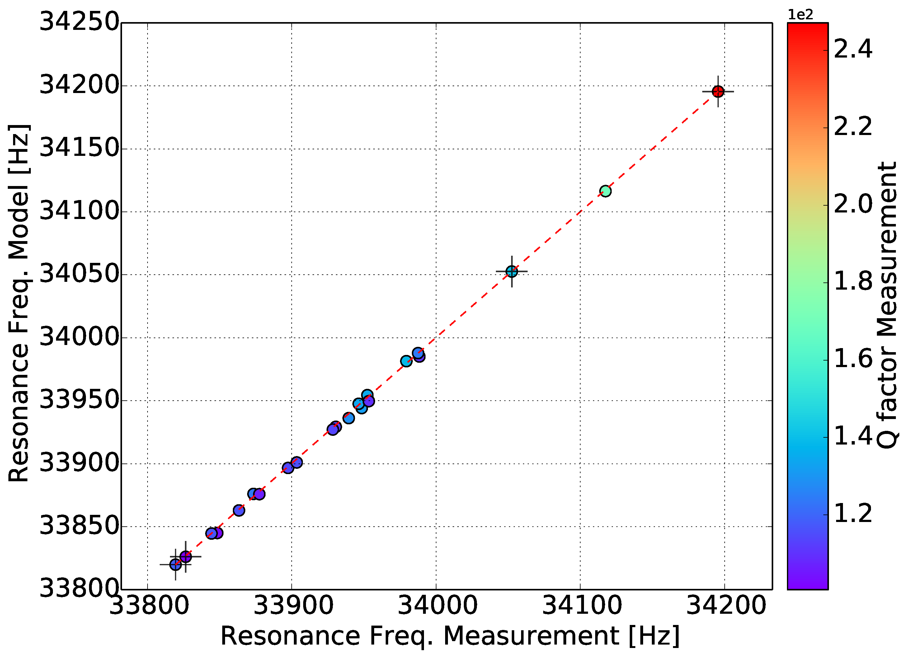
| Gas | (kHz) | |||
|---|---|---|---|---|
| 33.820 | 118.59 | 0.11 | 0.00 | |
| 33.863 | 116.02 | −0.20 | 0.17 | |
| 33.897 | 114.22 | −0.20 | −0.45 | |
| 33.931 | 112.61 | −0.34 | −0.71 | |
| 33.988 | 109.39 | −1.39 | −1.07 | |
| 34.196 | 247.12 | −0.12 | 0.27 | |
| 33.949 | 131.83 | −1.45 | −1.62 | |
| 33.979 | 138.97 | 1.32 | −1.95 | |
| 33.827 | 100.67 | −0.19 | 0.40 | |
| 33.929 | 113.74 | −0.28 | −1.26 | |
| 33.946 | 133.64 | 0.84 | −1.77 | |
| 34.053 | 141.21 | 0.18 | −0.65 | |
| 33.848 | 102.83 | −1.14 | 0.45 | |
| 33.952 | 134.66 | 1.27 | −2.08 | |
| 34.118 | 170.07 | −1.02 | 0.04 | |
| 33.904 | 115.78 | −0.81 | −0.39 | |
| 33.953 | 109.70 | −1.46 | −0.53 | |
| 33.844 | 116.96 | 0.05 | 0.03 | |
| 33.988 | 124.57 | 0.49 | −1.75 | |
| 33.874 | 123.72 | 1.08 | −1.32 | |
| 33.878 | 106.56 | −0.48 | −0.5 | |
| 33.940 | 128.14 | −1.09 | −1.16 |
References
- Kramer, A.; Paul, T. High-precision density sensor for concentration monitoring of binary gas mixtures. Sens. Actuators A Phys. 2013, 202, 52–56. [Google Scholar] [CrossRef]
- Rüst, P. Micromachined Viscosity Sensors for the Characterization of DNA Solutions. Ph.D. Thesis, Eidgenössische Technische Hochschule, ETH Zürich, Zürich, Switzerland, 2013. [Google Scholar]
- Kandil, M. The Development of a Vibrating Wire Viscometer and a Microwave Cavity Resonator for the Measurement of Viscosity, Dew Points, Density, and Liquid Volume Fraction at. Ph.D. Thesis, University of Canterbury, Chemical and Process Engineering, Christchurch, New Zealand, 2005. [Google Scholar]
- Bircher, B.; Duempelmann, L. Real-time viscosity and mass density sensors requiring microliter sample volume based on nanomechanical resonators. Anal. Chem. 2013, 85, 8676–8683. [Google Scholar] [CrossRef] [PubMed]
- Ghatkesar, M.; Rakhmatullina, E. Multi-parameter microcantilever sensor for comprehensive characterization of Newtonian fluids. Sens. Actuators B Chem. 2008, 135, 133–138. [Google Scholar] [CrossRef]
- Landau, L.D.; Lifshitz, E.M. Fluid Mechanics; Course of Theoretical Physics; Pergamon Press: Oxford, UK, 1987; Volume 6, p. 539. [Google Scholar]
- Boskovic, S.; Chon, J. Rheological measurements using microcantilevers. J. Rheol. 2002, 46, 891–899. [Google Scholar] [CrossRef]
- Goodwin, A. A MEMS Vibrating Edge Supported Plate for the Simultaneous Measurement of Density and Viscosity: Results for Argon, Nitrogen, and Methane at Temperatures from. J. Chem. Eng. Data 2008, 54, 536–541. [Google Scholar] [CrossRef]
- Xu, Y.; Lin, J.T.; Alphenaar, B.W.; Keynton, R.S. Viscous damping of microresonators for gas composition analysis. Appl. Phys. Lett. 2006, 88, 143513. [Google Scholar] [CrossRef]
- Rosario, R.; Mutharasan, R. Piezoelectric excited millimeter sized cantilever sensors for measuring gas density changes. Sens. Actuators B Chem. 2014, 192, 99–104. [Google Scholar] [CrossRef]
- Sell, J.; Niedermayer, A.; Jakoby, B. Simultaneous measurement of density and viscosity in gases with a quartz tuning fork resonator by tracking of the series resonance frequency. Proc. Eng. 2011, 25, 1297–1300. [Google Scholar] [CrossRef]
- Heinisch, M.; Reichel, E.; Dufour, I.; Jakoby, B. A resonating rheometer using two polymer membranes for measuring liquid viscosity and mass density. Sens. Actuators A Phys. 2011, 172, 82–87. [Google Scholar] [CrossRef]
- Smith, P.D.; Young, R.C.D.; Chatwin, C.R. A MEMS viscometer for unadulterated human blood. Measurement 2010, 43, 144–151. [Google Scholar] [CrossRef]
- Kuntner, J.; Stangl, G.; Jakoby, B.; Member, S. Characterizing the Rheological Behavior of Oil-Based Liquids: Microacoustic Sensors Versus Rotational Viscometers. IEEE Sens. J. 2005, 5, 850–856. [Google Scholar] [CrossRef]
- Lang, H.; Huber, F.; Zhang, J.; Gerber, C. MEMS technologies in life sciences. In Proceedings of the 2013 Transducers & Eurosensors XXVII: The 17th International Conference on Solid-State Sensors, Actuators and Microsystems (TRANSDUCERS & EUROSENSORS XXVII), Barcelona, Spain, 16–20 June 2013; IEEE: New York, NY, USA, 2013; pp. 1–4. [Google Scholar]
- Johnson, B.N.; Mutharasan, R. Biosensing using dynamic-mode cantilever sensors: A review. Biosens. Bioelectron. 2012, 32, 1–18. [Google Scholar] [CrossRef] [PubMed]
- Lu, J.; Ikehara, T.; Zhang, Y.; Mihara, T. Characterization and improvement on quality factor of microcantilevers with self-actuation and self-sensing capability. Microelectron. Eng. 2009, 86, 1208–1211. [Google Scholar] [CrossRef]
- Fantner, G.E.; Burns, D.J.; Belcher, A.M.; Rangelow, I.W.; Youcef-Toumi, K. DMCMN: In Depth Characterization and Control of AFM Cantilevers with Integrated Sensing and Actuation. J. Dyn. Syst. Meas. Control 2009, 131. [Google Scholar] [CrossRef]
- Vidic, A.; Then, D.; Ziegler, C. A new cantilever system for gas and liquid sensing. Ultramicroscopy 2003, 97, 407–416. [Google Scholar] [CrossRef]
- Naeli, K. Optimization of Piezoresistive Cantilevers for Static and Dynamic Sensing Applications. Ph.D. Thesis, Georgia Institute of Technology, Atlanta, GA, USA, 2009. [Google Scholar]
- Kucera, M.; Wistrela, E.; Pfusterschmied, G.; Ruiz-Díez, V.; Manzaneque, T.; Hernando-García, J.; Sánchez-Rojas, J.L.; Jachimowicz, A.; Schalko, J.; Bittner, A.; et al. Design-dependent performance of self-actuated and self-sensing piezoelectric-AlN cantilevers in liquid media oscillating in the fundamental in-plane bending mode. Sens. Actuators B Chem. 2014, 200, 235–244. [Google Scholar] [CrossRef]
- Blom, F.; Bouwstra, S.; Elwenspoek, M.; Fluitman, J. Dependence of the quality factor of micromachined silicon beam resonators on pressure and geometry. J. Vac. Sci. Technol. B 1992, 10, 19–26. [Google Scholar] [CrossRef]
- Hosaka, H.; Itao, K.; Kuroda, S. Damping characteristics of beam-shaped micro-oscillators. Sens. Actuators A Phys. 1995, 49, 87–95. [Google Scholar] [CrossRef]
- Kirstein, S.; Mertesdorf, M.; Schönhoff, M. The influence of a viscous fluid on the vibration dynamics of scanning near-field optical microscopy fiber probes and atomic force microscopy cantilevers. J. Appl. Phys. 1998, 84, 1782–1790. [Google Scholar] [CrossRef]
- Sader, J. Frequency response of cantilever beams immersed in viscous fluids with applications to the atomic force microscope. J. Appl. Phys. 1998, 84, 64–76. [Google Scholar] [CrossRef]
- Eysden, C.V.; Sader, J. Resonant frequencies of a rectangular cantilever beam immersed in a fluid. J. Appl. Phys. 2006, 100, 114916. [Google Scholar] [CrossRef]
- Van Eysden, C.A.; Sader, J.E. Frequency response of cantilever beams immersed in viscous fluids with applications to the atomic force microscope: Arbitrary mode order. J. Appl. Phys. 2007, 101, 044908. [Google Scholar] [CrossRef]
- Eysden, C.V.; Sader, J. Frequency response of cantilever beams immersed in compressible fluids with applications to the atomic force microscope. J. Appl. Phys. 2009, 106, 094904. [Google Scholar] [CrossRef]
- Hao, Z.; Erbil, A.; Ayazi, F. An analytical model for support loss in micromachined beam resonators with in-plane flexural vibrations. Sens. Actuators A Phys. 2003, 109, 156–164. [Google Scholar] [CrossRef]
- Zener, C. Internal Friction in Solids II. General Theory of Thermoelastic Internal Friction. Phys. Rev. 1938, 53, 90–99. [Google Scholar] [CrossRef]
- Lifshitz, R.; Roukes, M.L. Thermoelastic damping in micro- and nanomechanical systems. Phys. Rev. B 2000, 61, 5600. [Google Scholar] [CrossRef]
- Burns, D.J. A System Dynamics Approach to User Independence in High Speed Atomic Force Microscopy. Ph.D. Thesis, Massachusetts Institute of Technology, Cambridge, MA, USA, 2010. [Google Scholar]
- TÜV SÜD NEL PPDS for Windows v4.1.0.0. Available online: www.tuvnel.com/site2/subpage/software_solutions_ppds (accessed on 18 September 2015).
- Riesch, C.; Reichel, E.; Jachimowicz, A.; Schalko, J.; Hudek, P.; Jakoby, B.; Keplinger, F. A suspended plate viscosity sensor featuring in-plane vibration and piezoresistive readout. J. Micromech. Microeng. 2009, 19, 075010. [Google Scholar] [CrossRef]
© 2015 by the authors; licensee MDPI, Basel, Switzerland. This article is an open access article distributed under the terms and conditions of the Creative Commons Attribution license (http://creativecommons.org/licenses/by/4.0/).
Share and Cite
Badarlis, A.; Pfau, A.; Kalfas, A. Measurement and Evaluation of the Gas Density and Viscosity of Pure Gases and Mixtures Using a Micro-Cantilever Beam. Sensors 2015, 15, 24318-24342. https://doi.org/10.3390/s150924318
Badarlis A, Pfau A, Kalfas A. Measurement and Evaluation of the Gas Density and Viscosity of Pure Gases and Mixtures Using a Micro-Cantilever Beam. Sensors. 2015; 15(9):24318-24342. https://doi.org/10.3390/s150924318
Chicago/Turabian StyleBadarlis, Anastasios, Axel Pfau, and Anestis Kalfas. 2015. "Measurement and Evaluation of the Gas Density and Viscosity of Pure Gases and Mixtures Using a Micro-Cantilever Beam" Sensors 15, no. 9: 24318-24342. https://doi.org/10.3390/s150924318
APA StyleBadarlis, A., Pfau, A., & Kalfas, A. (2015). Measurement and Evaluation of the Gas Density and Viscosity of Pure Gases and Mixtures Using a Micro-Cantilever Beam. Sensors, 15(9), 24318-24342. https://doi.org/10.3390/s150924318