1. Introduction
In wireless sensor detection and classification applications, decision fusion has attracted great interests for its advantages in combining the individual decisions into a unified one without sending raw data to the fusion center [
1]. It provides a flexible solution for improving the classification accuracy without considering the classifiers used in local sensors [
2]. Besides, the data transmission amount is greatly decreased, thus energy consumption and bandwidth demand are significantly reduced [
3,
4]. Yet decision fusion has been proven valuable in both civilian [
5] and military [
6] applications for its advantages in survivability, communication bandwidth, and reliability considerations.
Target classification is a common problem in applications of sensor networks. In decentralized target classification systems with decision fusion, each sensor independently conducts classification operation and uploads its local decision to the fusion center, which combines these decisions into a global one. Compared with target classification with a single sensor, multiple sensor decision fusion has better performance in classification accuracy, anti-noise, and reliability [
7].
Fundamentally, multiclass decision fusion in WSNs is a problem of combining the ensemble decisions of several different classification systems. Existing methodologies can be concluded into two categories: hard decision (HD) fusion [
8] and soft decision (SD) fusion [
9]. In HD schemes, each sensor sends their hard decisions to fusion center,
i.e., clearly declare which class the target belongs to. The fusion center makes a decision according to some fusion rules, like counting rules [
10], weighted sum [
11], Neyman–Pearson criterion [
12], or the max-log fusion [
13]. The typical fusion HD scheme is the majority voting rule [
14], though it has great advantage in easy implementation, the low fusion accuracy decreases it practicability. In SD schemes, local decisions are usually represented by values between 0 and 1 and the fusion operation is always conducted based on some decision fusion theories, including Bayesian fusion [
15], Fuzzy logic [
16] and belief function theory [
17]. Except the above mentioned fusion schemes, many other centralized fusion approaches have been proposed, such as Decision Template [
18], Bagging [
19], and Boosting [
20]. Some centralized fusion approaches, like Bagging and Boosting, have been proven to always perform better than other decentralized classifier ensemble approaches. However, centralized fusion approaches require sensor nodes to send raw data to the fusion center, a way consumes two much energy in data transmission, thus it is not applicable in decentralized target classification scenario in WSNs.
Another promising way to improve fusion performance is designing decision fusion schemes with Multiple-Input Multiple-Output (MIMO) technique, which enables sensors to transmit data to the fusion center via multiple access channels [
21,
22]. Benefit from the diversity gain in the fusion center, these MIMO based fusion schemes have been proven to have much better performance in sensing performance [
23,
24], anti-fading [
25,
26,
27], bandwidth demand [
28], and energy efficiency [
29,
30,
31]. Even so, in MIMO based schemes, fundamental fusion rules underlying the decision fusion operation still play a central role in determining the overall sensing performance in the fusion center. Moreover, decision fusion in WSNs are usually designed based on wireless signal detection and transmission models [
32,
33,
34,
35], thus they may not be compatible with the multiclass classifier decision fusion problems.
As such, in this paper, we aim to design a decentralized decision fusion rule to improve overall classification performance while uploading data as little as possible. We focus on using belief function theory to address the decentralized decision fusion problem in WSNs with ideal error-free reporting channels. The belief function theory, also known as the Dempster-Shafer (DS) evidence theory, provides a flexible solution dealing with multisource information fusion problems, especially problems with uncertainty [
36]. However, existing belief function based approaches have the two following disadvantages in practical applications:
(1) Poor compatibility with other classifiers. Different classification algorithms have their own advantages. It is hard to say which one is the best choice for a specific task, thus different classifiers may be used in different sensors, especially in heterogeneous WSNs. However, the prerequisite of applying belief function to addressing the information fusion problem is constructing rational basic belief assignments (BBAs), which are always constructed by specifically designed mass constructing algorithms, but have no business with other classification algorithms.
(2) Complex combination operation and energy inefficiency. The BBA combination operation is the key capacity enabling belief function theory dealing with fusion problems. However, the complex BBA combination operation requires each sensor node to upload the whole BBA structure to the fusion center, a way that consumes higher energy in data transmission than other fusion schemes, especially compared with HD fusion schemes. Moreover, the complex computation of combination operation adds the burden in system overhead to sensors and fusion center.
In conclusion, the main contributions include the following three aspects:
(1) A BBA construction algorithm based on the training output confusion matrix and decision reliability is proposed. The proposed mass construction algorithm has a strong compatibility without considering the classifiers used in the classification process. Compared with the probability-only based fusion schemes, the proposed approach is more reasonable because the constructed BBAs are adjusted by real-time observations.
(2) A new decision fusion rule based on belief function theory is proposed. By using Dempster’s combinational rule, we derive the explicit expression of the unified BBA in fusion center, and then a new simple fusion rule is derived. As a result, the complex BBA combination operation is avoided. Also, energy consumption for data transmission is reduced because there is no need to upload the whole BBA structure to fusion center.
(3) We test the proposed fusion rule with both a randomly generated dataset and a vehicle classification dataset. Experimental results show the proposed rule outperforms the weighted majority voting and naïve Bayes fusion rules.
The remainder of this paper is organized as follows:
Section 2 gives a brief introduction of preliminaries of belief function theory. The proposed belief function based decision fusion approach is presented in
Section 3.
Section 4 provides the experimental results along with the analysis. Finally
Section 5 concludes this paper.
3. Belief Function Based Multi-Class Decision Fusion
3.1. System Model
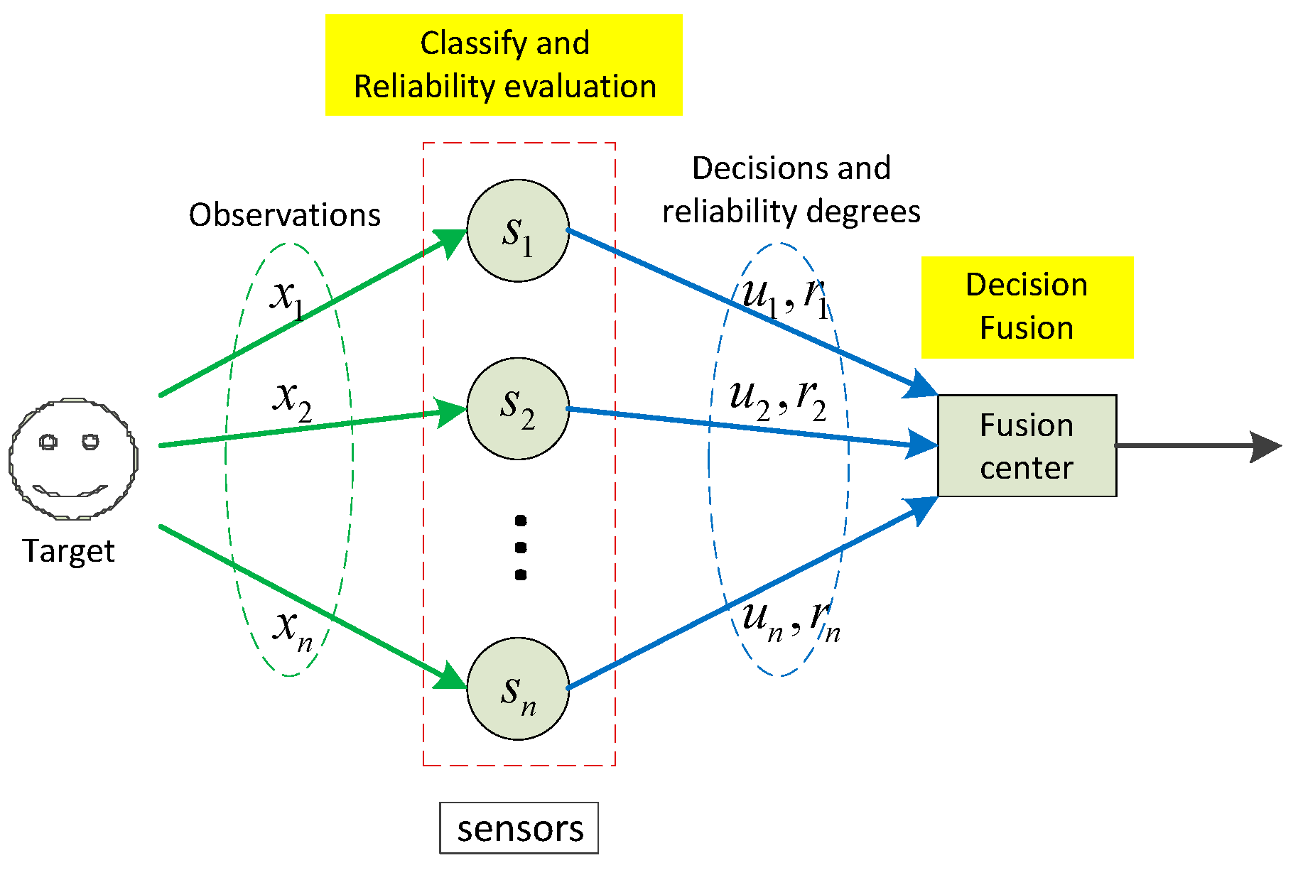
The system model is depicted in
Figure 1. Suppose there is a distributed sensor network with
sensors. All sensors are assumed to be mutually independent and they can use any classifiers for the classification task. For a target with
possible classes (labels), the
n sensors conduct local classification operations according to their own observations
, and we set the corresponding hard decisions are
, in which
. Also, we define the reliability degrees of the decisions as
, which can be computed according to the corresponding real-time observations
. With the received hard decisions and reliability degrees, the fusion center then conducts the decision fusion operation with the proposed fusion rule. At last, the final decision is made by choosing the class (label) with the maximum BBA. Note that the decision fusion operation in the fusion center is conducted according to a simple fusion rule induced by the belief function theory, thus the complex BBA construction and BBA combination operations are avoided. In the following subsections, the detailed local classification, reliability evaluation, and decision fusion processes will be provided.
Figure 1.
System model of the proposed decision fusion approach.
Figure 1.
System model of the proposed decision fusion approach.
3.2. Classification and Reliability Evaluation
In local sensors, the classification process can be made by any appropriate recognition algorithms. For a multi-class pattern recognition problem, we assume that all the local classifiers are well trained and the training output confusion matrices are previously known to the fusion center, i.e., the fusion center maintains a confusion matrix for each sensor. We don’t consider the details of its classification operation, such as signal segmentation, feature extraction, and classification algorithm. For sensor , when given a new observation, it conducts the classification operation and makes it local decision . For decision , we define as its corresponding reliability degree. In this paper, we propose a distance based algorithm to calculate the reliability degree for each local decision.
The best way to calculate the reliability of a classifier’s output is designing a specific algorithm measuring the similarity of the output before the final decision is made [
40]. For example, if we want to know the reliability of a local decision when the classifier is an artificial neural network (ANN), the output before decision making in the output layer can be used as the basis for reliability evaluation. For another example, when using
k-NN classifier for classification, the distance between the object and
k nearest neighbors in sample set of each class label can be exploited to measure the reliability.
Herein in this paper we also provide a more general method to evaluate the reliability degree for each local decision. The method follows the basic assumption that, when the object to be classified has a smaller distance to the sample set of a class label, then the decision result is more reliable. On the contrary, when the distance is large, the reliability is low. This distance can be computed by any appropriate distance definitions, such as Euclidean distance, Mahalanobis distance, Hamming distance, and the like. Also, the chosen samples for distance calculation can be the whole sample set, or the k nearest neighbors to the object. Usually, the distance definition is Euclidean distance and the chosen samples are one to five nearest neighbors to the object.
For a sensor
, denote its training set as
, where
is a
N-dimensional vector containing
N data samples. Given a new observation
, the distance to each sample set can be calculated and we denote
as the distance between
and sample set
. Let the local decision
and its corresponding distance is
, we define the relative distance
as
If the relative distance
is large, it means that we have sufficient confidence to confirm that
is not the class label of the target. On the contrary, if
is small, the possibility that
is class label will be large. By using an exponential function, the distance can be transferred into BBAs [
41]. Also, we use an exponential function to map distance into reliability. Similar to the transferring function in [
41], we define the reliability measurement of decision
as
where
and
are positive constants and they are associated to the relative distance. Together with the local decision
, obtained reliability measurement
will be uploaded to the fusion center. In the fusion center, the received pattern
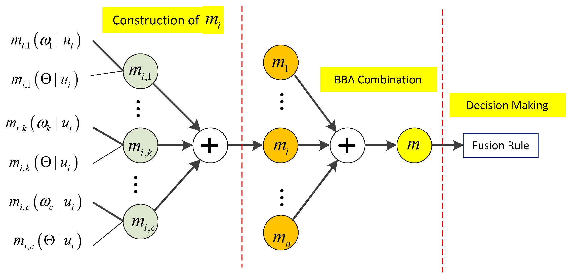
will be used as the basis for the global decision making. In next subsection, we will elaborate the detailed derivation of the proposed decision fusion rule, including BBA construction, BBA combination and decision making, as illustrated in
Figure 2.
Figure 2.
Derivation process of the proposed approach, in which denotes the Dempster BBA combination operation, is the constructed BBA of sensor , is the global BBA of all sensors.
Figure 2.
Derivation process of the proposed approach, in which denotes the Dempster BBA combination operation, is the constructed BBA of sensor , is the global BBA of all sensors.
3.3. BBA Construction
Reasonable BBAs are the prerequisite when applying belief function to address data fusion problems. With the received patterns
from sensors, a set of probability vectors can be obtained from the corresponding confusion matrix of sensor
. For decision
, we have the probability vector
, in which
is the conditional probability of class label
when the local decision is
. Although belief and probability are two different concepts, but one thing is certain that, a larger probability will be accompanied by a larger belief. In the contrary, a smaller belief value corresponds to smaller probability value. This distinct evidence can be postulated to transfer each probability
into a BBA
over the frame of discernment
, as given by
for the compound class
, we define its BBA as
thus for any other classes
, their BBAs equal to 0, that is
With the obtained BBAs
, the BBA
with respect to
can be calculated by
where
denotes the BBA combination operation. For convenience, we denote
as
for short. Note that the value of
always not equals to 1,
i.e., for a decision, the sum of probability of detection and probability of false alarm does not equal 1. According to Dempster’s combinational rule, the explicit expression of
is given by
where
designates the conflict degree of BBAs
, and it equals to
Combined with Equations (11) and (12), we have the following relationship between BBA
and
3.4. BBA Combination
After the BBA construction process, we obtained BBAs
. The next step is combining these BBAs into a unified one. We assume that all BBAs in
are mutually independent, given two BBAs
and
, for class label
, we have
For compound class
, we have
Equations (17) and (18) indicate that, when given
n BBAs, the combined result follows a certain rule. Thus we have reasons to assume that the unified combination result in the fusion center is
Proof: The above proposition can be proved via mathematical proof of induction. Apparently, given
n+1 sensors, we have
Then we just have to prove Equation (19) is true for any sensor number. Assume that Equation (17) is true with
n sensors, when sensor number is
n + 1, we have
Consequently, we have proved that equation is true with any sensor number.
3.5. Decision Making
In the above subsection, we have derived the explicit expression of the unified BBA in the fusion center, as given in Equations (19) and (20). The final decision can be made by choosing the label with maximum belief assignment, as given by
Actually, there is no need to consider the conflict degree
because it is the same for all class labels, thus the above decision rule can be simply expressed as
Also, the above decision making rule is equivalent to
With the above decision making rule, the complex BBA combination operation is avoided, thus the system overhead is reduced. The pseudocode of the proposed approach is shown in the Algorithm 1. Note that the classification performance, i.e., the training confusion matrix of each local sensor is default known to the fusion center. This may be realized by sending the confusion matrix to fusion after the training process. Another way is that the classifiers and sample data can be previously trained in the fusion center before they are embedded into the sensors, thus the classification performances of the sensors are also known to the fusion center.
| Algorithms 1 Belief function based decentralized classification fusion for WSN |
1: event target is detected by n sensors do
2: for each observation is received by sensor do
3: classify the object and obtain local decision
4: calculate local reliability measurement by (8)
5: send pattern to fusion center
6: end for each
7: end event
8:
9: event fusion center receives uploading from sensors do
10: for each received pattern do
11: find the probability vector
12: end for each
13: make final decision
14: end event |
4. Experimental Results
In experimental section, two experiments will be conducted. The first one is used to evaluate the fusion performance by using a randomly generated dataset, whose sensor number and the sensors’ classification accuracies can be artificially changed. Therefore, the performance comparison results can be provided with changing sensor number or sensor accuracy. The next one is testing the performance of the proposed fusion approach by using the sensit vehicle classification dataset [
42]. In the two experiments, all sensor nodes are all assumed to be equipped with sufficient computational capacity to underlay the local classification and reliability evaluation operation. We assume that the reporting channel is ideally an error-free channel. Also, we don’t consider how to quantify the reliability degree when it is transmitted to the fusion center. Thus the information of each sensor will be sent to the fusion center without distortion.
Considering the computation complexity, the following two easy implementing algorithms are used as the local classifiers:
k-nearest neighbors (
k-NN) algorithm and extreme learning machine (ELM) neural network. The detailed introduction of k-NN and ELM algorithms can be found in [
43,
44], respectively. For performance comparison, the following two conventional decision fusion approaches will be used.
Naïve Bayes: the naïve Bayes fusion method assumes that all decisions are mutually independent. In binary fusion systems, this fusion method is regarded as the optimal fusion rule. In a fusion system with
M sensors, denote
as the probability of label
k corresponding to decision
, the fusion decision is made by choosing the label with maximum fusion statistic, as given by
Weighted majority voting: denote
as the decision on label
of sensor
. When the target belongs to
, we have
and
. In weighted majority voting, decision
is weighted by an adjusting coefficient
, and the decision is made by
weight
can be calculated by
where
is the classification accuracy of sensor
. Apparently, a sensor with higher accuracy will be assigned a larger weight. Always, this rule performs better than the simple majority voting rule.
4.1. Experiment on Randomly Generated Dataset
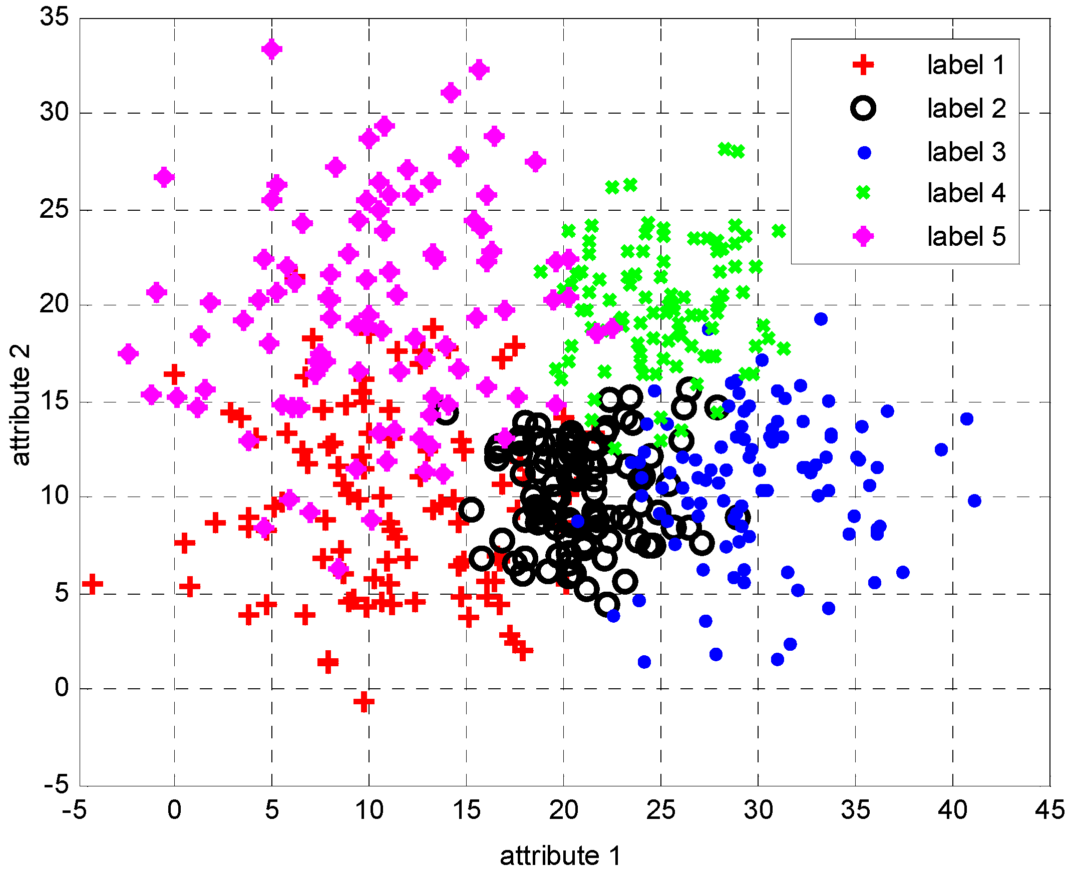
In this test, our goal is to evaluate the performance variation of the three fusion approaches with different sensor numbers or local classification accuracies. Since the local classification accuracies of datasets in reality are fixed, the randomly generated the dataset must be used if we want to evaluate the performance with changing sensor classification accuracies. In this test, we randomly generated the dataset by using Gaussian random number generation function. The target class label number is fixed as five, each sample data is assumed to have two randomly generated attributes following different Gaussian distributions.
As shown in
Table 1,
is a coefficient changing the standard deviations of the sensor data attributes. For example, the two attributes of class label
follow the two Gaussian probability density functions (pdf):
and
, respectively. Apparently, coefficient
determines the sensor classification accuracies,
i.e., a larger
brings lower classification accuracy.
Figure 3 gives an example depiction of the randomly generated sample data.
Table 1.
Data generation parameters.
Table 1.
Data generation parameters.
| Label | | | |
|---|
| 10 | 10 | 5 |
| 20 | 10 | 3 |
| 30 | 10 | |
| 25 | 20 | 3 |
| 10 | 20 | 5 |
Figure 3.
Example of a randomly generated dataset, each class label has 100 samples and the coefficient equals to 1.
Figure 3.
Example of a randomly generated dataset, each class label has 100 samples and the coefficient equals to 1.
Since the dataset is randomly generated each time, we repeat it i20 times to obtain the average classification accuracy. In each repetition, to know the posterior probabilities of the training process, 1500 samples and 500 samples are respectively generated as the training data set and validation data set, in which each class label has the same sample number, i.e. each of them has 300 train samples and 100 valid samples. After training process, the classifier used in each sensor is also obtained. Subsequently, 1000 samples are randomly generated as new observations. In these new observations, the class label of each observation is randomly selected, thus the number of each class label is approximated to 200. Next we classify the new observations by using the classifiers obtained in the training process. At the same time, the reliability degree of each decision is calculated by using Expression (8). Next, the local decisions and their corresponding reliability degrees are uploaded to fusion center and the final decision is finally made according to Equation (23).
As aforementioned, the following two classifiers are used for classification in sensors:
k-NN and ELM neural network. If there are no specific instructions, the
k nearest neighbors used in
k-NN is 3. In the reliability evaluation process, the nearest neighbor number used for calculating distances is also fixed as 3. The number of hidden neurons in ELM is 50 and the activation function is “radbas” function. For the weighted majority voting rule, the weight of each decision is calculated by
. In Expression (8), parameter
is fixed as 1.5, and parameter
corresponding
ith decision
is calculated by
The following three approaches are used for performance comparison: the proposed belief function fusion approach, naïve Bayes fusion, and majority voting fusion. Define classification accuracy as the total number of correct classifications over the number of trials. The classification accuracy results with changing
values are shown in
Figure 4. The used classifiers in
Figure 4a and
Figure 4b are
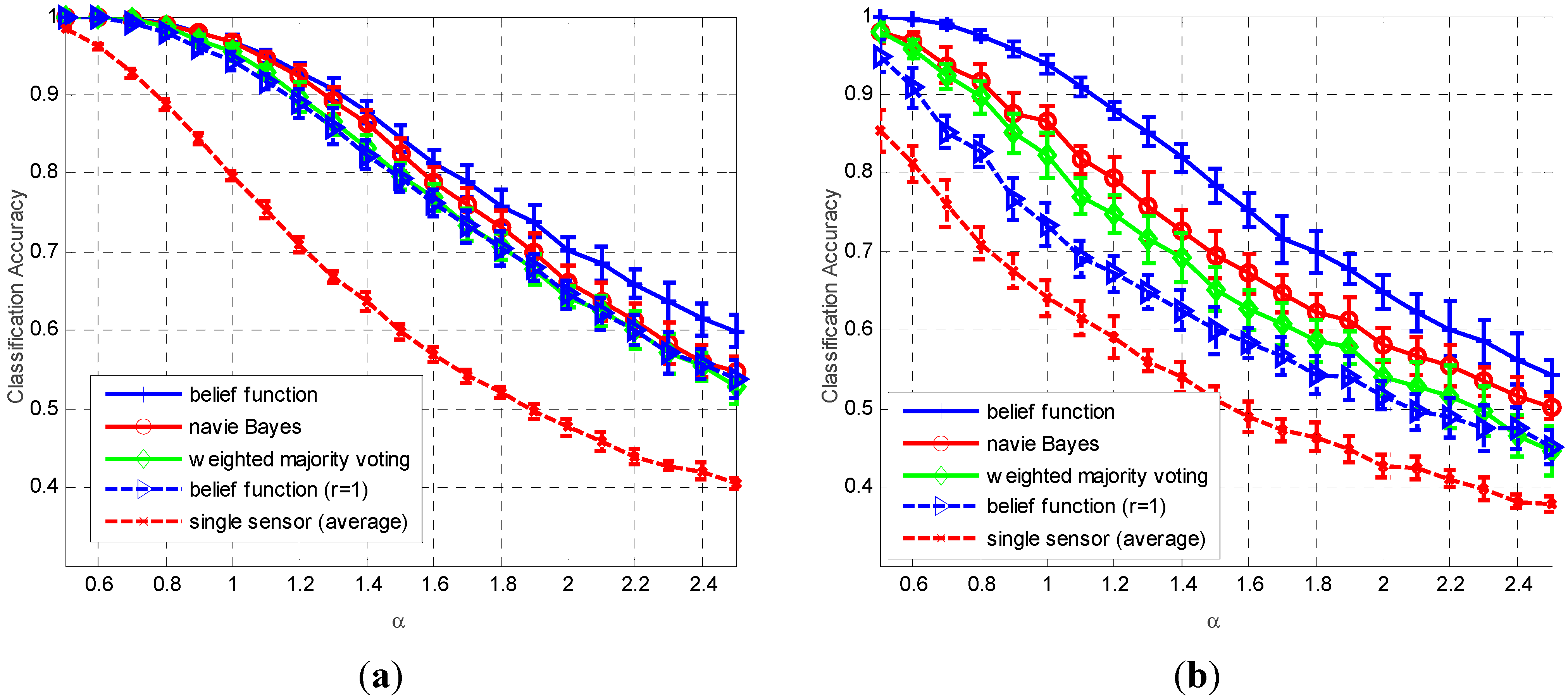
k-NN and ELM neural network, respectively. The sensor number is fixed as 5. In
Figure 4a, when the value of coefficient
increases from 0.6 to 2.5, the average classification accuracies of the local sensors decrease from 0.97 to 0.4, along with the decreasing of the classification accuracies of fusion results. In
Figure 4b, the average sensor classification accuracies and final fusion accuracies also decrease with the increasing of
value. We can find that the classification of the ELM neural network is usually lower than the
k-NN classifier, especially when
is smaller than 1.4, thus obviously the classification accuracies of the three approaches when using ELM classifier are lower than the fusion accuracies of
k-NN classifier. Apparently, we can observe that the proposed belief function based fusion approach always outperforms the naïve Bayes fusion and weighted majority voting fusion approaches, especially for the classifiers with lower classification performances.
Figure 4.
Average classification accuracy (plus and minus one standard deviation) as a function of values, obtained by 20 repetitions. The sensor number is fixed as M = 5 and the used classifiers in subplots (a,b) are k-NN and ELM neural network, respectively.
Figure 4.
Average classification accuracy (plus and minus one standard deviation) as a function of values, obtained by 20 repetitions. The sensor number is fixed as M = 5 and the used classifiers in subplots (a,b) are k-NN and ELM neural network, respectively.
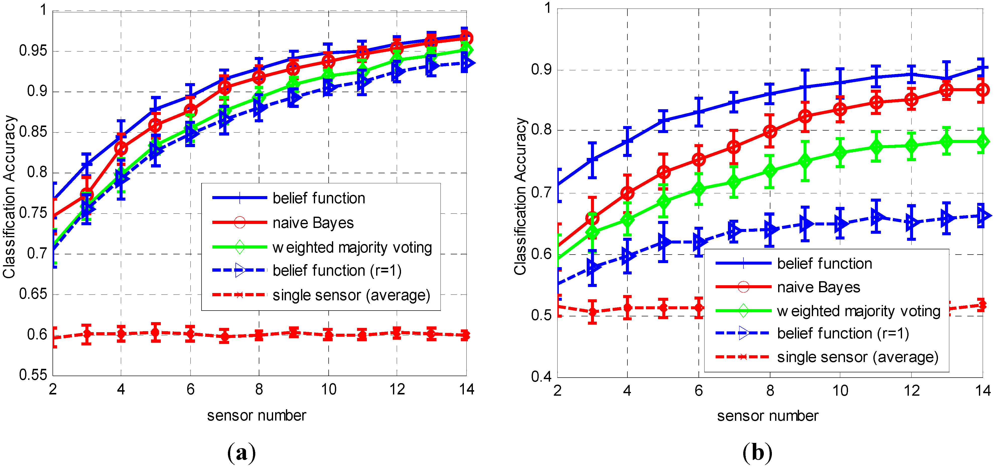
The performance comparison results with changing sensor numbers are plotted in
Figure 5. In this test, the value of coefficient
is fixed as 1.5. The results also show that the proposed approach always outperforms than the other two approaches with changing sensor numbers. The accuracy improvement is more significant when sensor number is less than 7.
The proposed fusion approach has a very similar form to the naïve Bayes fusion rule, but they have distinct difference in fusion accuracies. As shown in
Figure 4 and
Figure 5, when the decision reliability in each sensor is fixed as 1, the classification accuracies of the fusion results are always lower than the other two approaches. This result indicates that the reliability evaluation method is the key factor influencing the fusion results’ classification accuracies of the proposed rule.
Figure 5.
Average classification accuracy (plus and minus one standard deviation) as a function of sensor number, obtained by 20 repetitions. The value of coefficient is fixed as 1.5 and the used classifiers in subplots (a,b) are k-NN and ELM neural network, respectively.
Figure 5.
Average classification accuracy (plus and minus one standard deviation) as a function of sensor number, obtained by 20 repetitions. The value of coefficient is fixed as 1.5 and the used classifiers in subplots (a,b) are k-NN and ELM neural network, respectively.
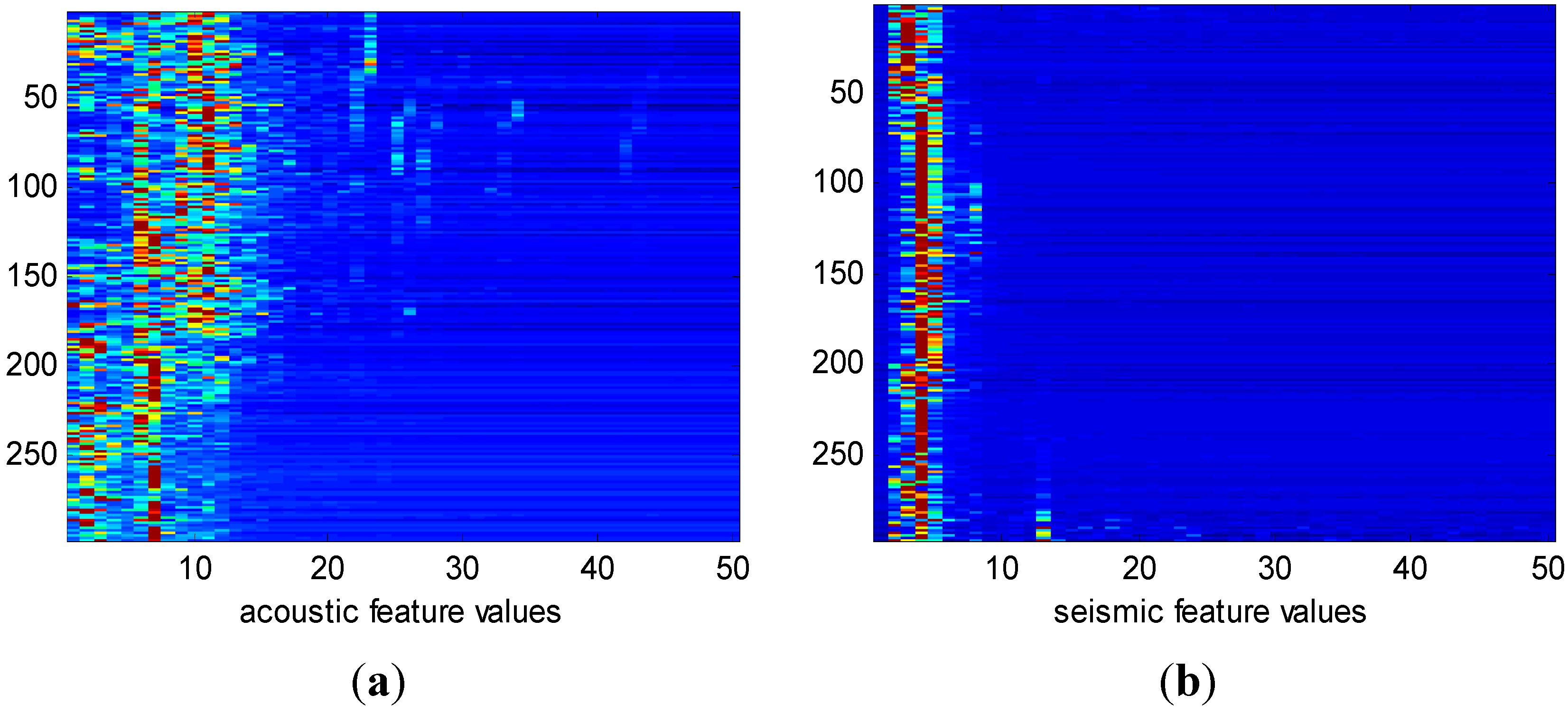
Figure 6.
Image plot of extract features. Subplots (a,b) are features extracted from acoustic signals and seismic signals, respectively. The vehicle type is AAV and each of the subplots has 297 features.
Figure 6.
Image plot of extract features. Subplots (a,b) are features extracted from acoustic signals and seismic signals, respectively. The vehicle type is AAV and each of the subplots has 297 features.
4.2. Experiment on Vehicle Classification
In this test, we use the
sensit vehicle classification dataset collected in real application, in which the wireless distributed sensor networks are used for vehicle surveillance. There are 23 sensors deployed in total along the road side listening for passing vehicle. When vehicles are detected, the captured signal of the target vehicle is recorded for acoustic, seismic, and infrared modalities. The signal segmentation and feature extraction process can be found in [
42]. In our test, 11 sensor nodes are selected for vehicle classification. The target vehicle may belong to the following two types: Assault Amphibian Vehicle (AAV) and DragonWagon (DW). Features extracted from the recorded acoustic and seismic signals are used for vehicle classification. Examples of the extracted features are shown in
Figure 6.
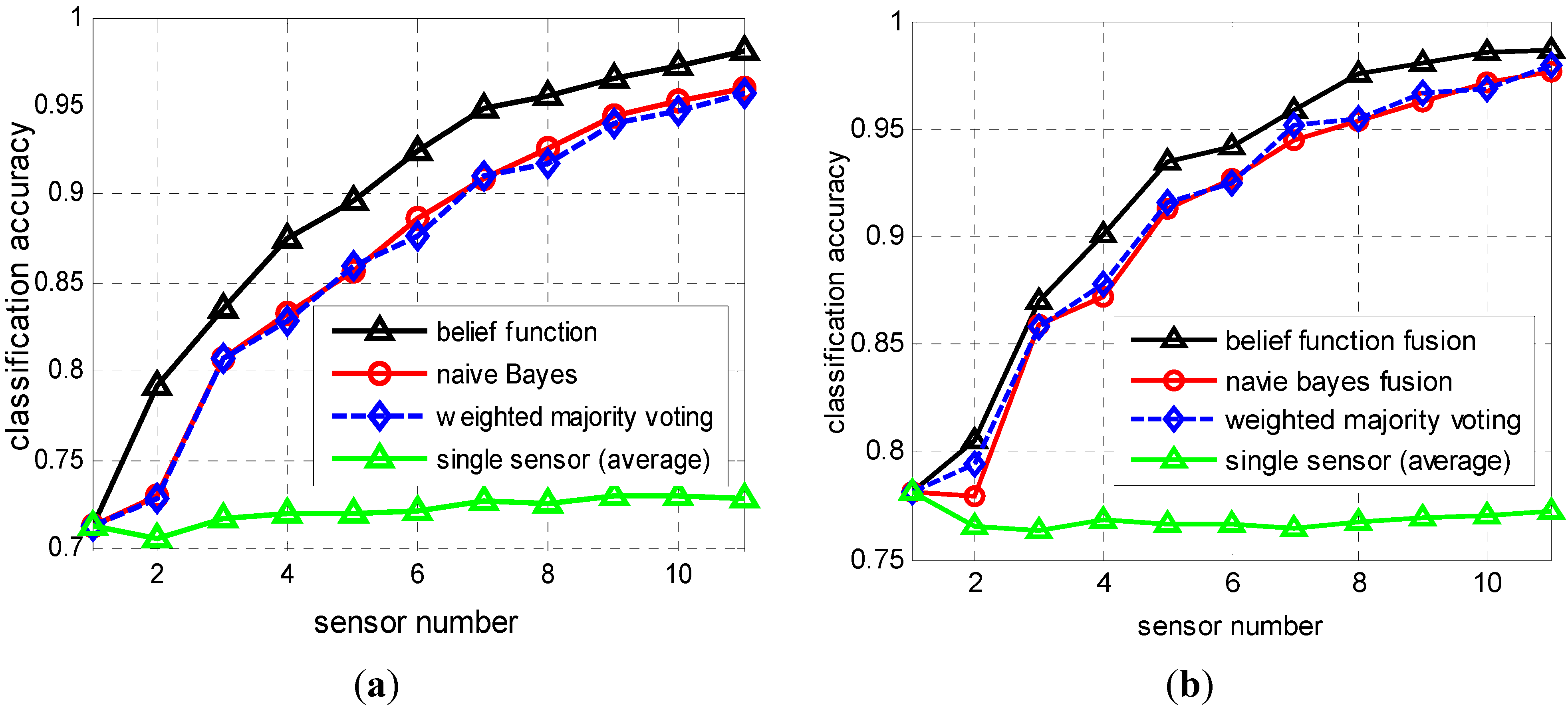
Figure 7.
Classification accuracy as a function of sensor numbers. Classifiers used in subplots (a,b) are k-NN and ELM neural network, respectively.
Figure 7.
Classification accuracy as a function of sensor numbers. Classifiers used in subplots (a,b) are k-NN and ELM neural network, respectively.
The experiment procedure is the same with the previous experiment, thus we don’t repeat it again. The difference is that, when the training samples are given, the classification accuracy of sensor nodes is fixed as a constant value. In this test, the “
k” used in
k-NN classifier and reliability calculation are all equal to 1. The two parameters
and
in Expression (8) are fixed as 1 and −0.5, respectively. The hidden neuron number of ELM neural network is 50 and the activation function is also the “radbas” function. The accuracy comparison of fusion results are provided in
Figure 7. We can observe that the performance improving of the proposed approach for
k-NN classifier is better than the ELM classifier. But the final fusion accuracy of ELM is higher than
k-NN classifier when the sensor number is the same. Again, we easily conclude that the proposed approach has better performance in improving the fusion accuracy for distributed target classification applications.


