1. Introduction
Large-scale shape measurement of objects is of great importance in numerous application fields, including cultural heritage protection, film-making, automotive parts, aerospace aircraft, fan blade manufacturing and so on [
1,
2,
3,
4]. In most cases, the three-dimensional (3-D) data of an object are desirable because it is necessary for its quantitative analysis. However, as the size increases the measurement accuracy decreases and difficulty increases, especially for irregular shapes.
In the past decades, several acquisition methods have emerged and have been commercialized [
5,
6,
7,
8]. Articulated arms, laser trackers, total stations and theodolites can be used to derive high-precision 3-D coordinates, but they are all single point measurement devices. For example, the laser tracker measures the relative position by means of a laser interferometer and a beam-steering mirror using optical encoders. The light source is split into two beams. One beam is used as a reference, and the other beam is reflected back from a retro-reflector. The laser beam hits the retro-reflective target off-center, and it is then reflected back parallel to the incident beam. A sensor measures the displacement [
9,
10]. Consequently, only a point can be measured every time, therefore the measurement efficiency is too low.
Figure 1.
(a) The original point cloud; (b) Reconstruction surface; (c) Error distribution diagram.
Figure 1.
(a) The original point cloud; (b) Reconstruction surface; (c) Error distribution diagram.
To validate that these devices are not suitable for shape measurement, we performed an experiment with a laser tracker to obtain the surface geometry data of a pipe with a diameter of 690 mm, a total length of 1875 mm and a bend curvature radius of 3200 mm. It took 6 h in all to obtain 50 thousands 3-D points, as shown in
Figure 1a. However, the surface reconstruction, as shown in
Figure 1b, has obvious distortions and the maximum error is up to 110.74 mm, as shown in
Figure 1c. These errors are mainly attributed to the sparse data. Therefore, it is difficult for single point devices to be used in the field of surface high-density measurement.
Optical scanning sensors have been proven to be both an accurate and cost-effective alternative to deliver more geometry and appearance information for small objects. They operate on the basis of optical triangulation; that is, a light source (
i.e., a single laser spot or a laser stripe) scans an object surface while its reflection is being recorded by one or more CCD cameras. The resulting distance is a function of the CCD inclination angle and the base-length defined between the CCD camera and the laser sensor [
11,
12]. However, the field of view in a certain station is generally limited to only a few hundred millimeters, so when measuring a large-scale workpiece, the scanning sensor must be placed at different stations around the workpiece. Then the point clouds from the different stations should be registered into a global coordinate system by the corresponding points in the overlapping areas. What’s more, as the size increases, many scans are needed and the number of registrations rises [
13]. Thus, optical scanning turns out to be a time consuming and inaccurate process. Consequently it is difficult to obtain the whole morphology and 3-D coordinates of an object with only one certain kind of measuring instrument, so a combination of global position and local measurement is generally used. There have already been some reports on this. Paoli introduced a method based on the integration of a robotic system with an optical scanning sensor for automating the measurement process of built hull yacht shapes [
14]. Nevertheless, the measurement range was limited by the length of the robotic arm. Shi proposed a 3-D measurement method by combining an optical scanning sensor with a laser rangefinder. The laser rangefinder was fixed on a guide rail, and the scanning sensor could slide on the guide rail to perform partial section measurement [
4]. However, for measuring large-scale workpieces it is necessary to design and manufacture a long guide rail with high precision, so the cost will be greatly increased. To expand the measurement range, Hexagon Metrology, Inc. (Nacka Strand, Sweden), proposed a method of combining a laser tracker and a T-scan, which has a reflector and can be detected by the laser tracker. Nonetheless, the T-scan must always be tracked by the laser tracker, so the scanning speed is constrained [
15]. In summary, the existing methods are not the best solutions for large-scale shape measurement, so we propose herein a method involving the combination of a handheld laser scanning sensor and a laser tracker. Our method does not need any mechanical device, and the measurement range is expanded to tens of meters. What’s more, the measurement data is so abundant that the surface shape can be described in detail.
However, only from these points, the surface and geometry information are not available, so we must reconstruct the surface according to these point cloud data. After the surface reconstruction, many studies, such as quality control, non-destructive testing (NDT), product development and numerical simulation including finite element analysis and computational fluid dynamics analysis can all be carried out.
Considerable research has been done for many years on surface models. The Renault engineer Bézier proposed a method to define curves and surfaces with a control polygon to control the curve and surface shape. However, local modification is not supported by the Bezier method, and the continuity of the curve and surface is poor [
16]. Gordon and Riesenfeld proposed B-spline curves and surfaces to describe shapes, which overcame the disadvantages of the Bezier methods [
17]. However, conic and elementary analytic surfaces cannot be expressed accurately. Syracuse presented the Non-Uniform Rational B-Spline (NURBS) method to offer a common mathematical form for both standard analytical shapes (e.g., conics) and freeform shapes [
18]. Recently, NURBS was commonly used in computer graphics for generating and representing curves and surfaces. It offers great flexibility and precision for handling both analytic (surfaces defined by common mathematical formulae) and modeled shapes.
In this work, we construct the large-scale shape measurement system by the combination of local scanning and global positioning. A handheld laser scanning sensor provides precise measurements of high-density points, although, its measurement range is about a few hundred millimeters. Together with the large measurement range of the global position sensor, a laser tracker, the combination of two sensors could compensate each other to guarantee the efficiency, the data density and the precision at the same time. The multiple sensors will generate a mass of data. To transform the data into a global coordinate system, we adopt a multi-sensor data fusion method to decrease the transformation errors. Besides the point cloud data acquisition, the surface reconstruction is important for the shape measurement. In this paper, we propose a method to reconstruct the surface of a large-scale gear rim. It is significant in practical measurement field. Finally, the error analysis and synthesis of the entire system is established.
2. Description of the Combined System
2.1. System Design
As shown in
Figure 2, the described system is made up of a handheld laser scanning sensor, a laser tracker, used as a position sensor, and the PC software. Compared with traditional scanning sensors, the handheld laser scanning sensor is more suitable for performing local scanning. Without the limitation of the external mechanical device, the scanner possesses six degrees-of-freedom in motion to eliminate the blind areas, and meanwhile, the scanning process is simplified.
Figure 2.
Schematic of the combined system.
Figure 2.
Schematic of the combined system.
In this paper, we choose a MAXscan device (Creaform, Inc., Québec, QC, Canada), for acquiring the local dense point clouds. It is composed of a class-II laser diode that projects a crosshair over the surface to digitize, and two synchronized cameras with a resolution of 0.1 mm, that capture the image of projections at a high rate. As the relative position of the laser diode and two cameras is calibrated, a triangulation-based algorithm enables the acquisition of the coordinates of the points. Its accuracy is up to 0.05 mm, at a measuring speed of 48,000 scans per second. Therefore, it’s possible to obtain all the surface shape details of complex objects.
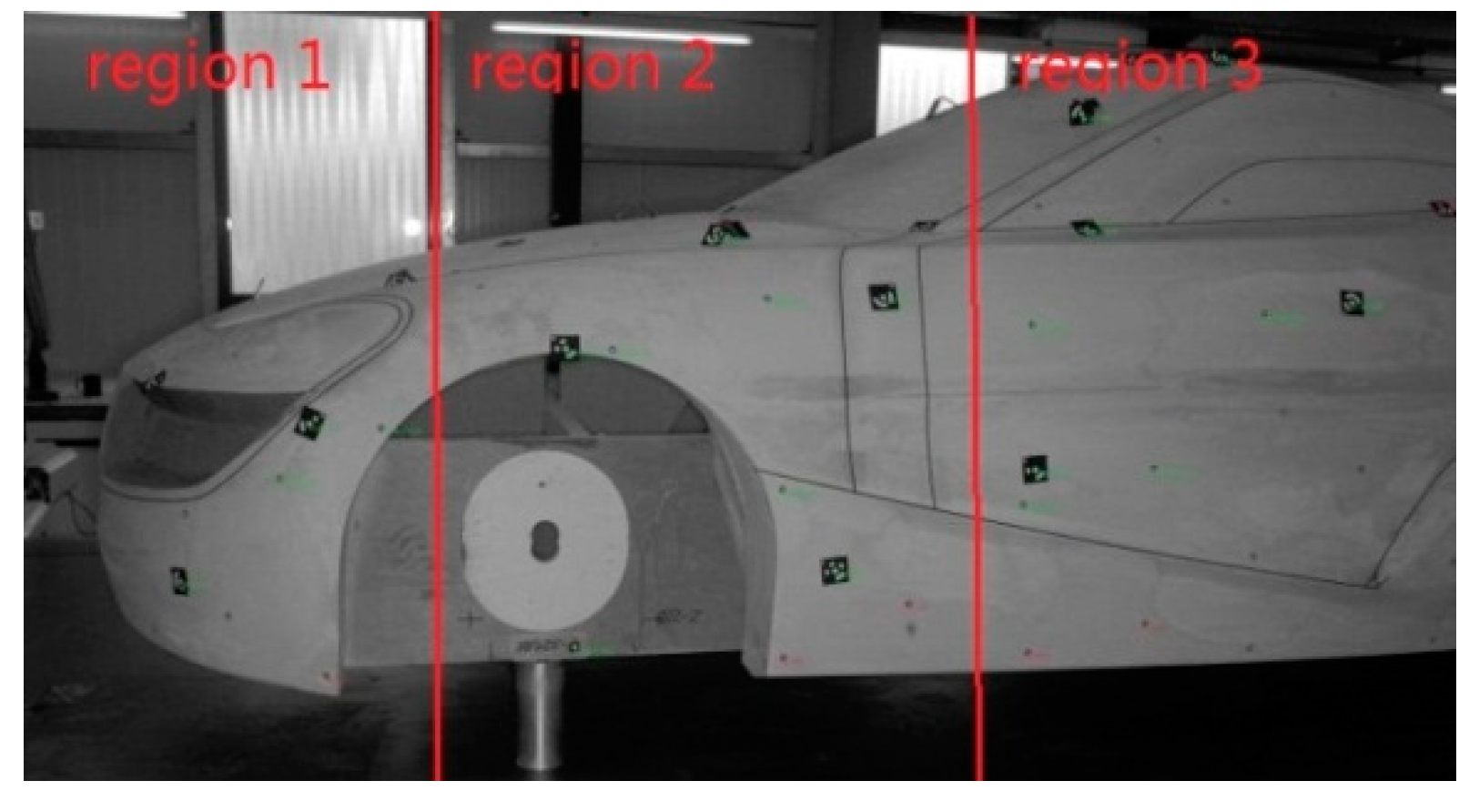
Compared with the total station, the theodolite and the digital photogrammetry system, the measurement accuracy of the laser tracker is higher, and the measurement range is larger. What’s more, the laser tracker is able to link multiple discontinuous partial regions of interest over a large volume into the global coordinate system. For example, the measured volume is so large that it will be separated into several small regions to decrease the accumulated errors in the scanning process. As shown in
Figure 3, the bodyshell is divided into three regions. If we are only interested in region 1 and region 3, we just scan region 1 and region 3 and transform them into the global coordinate system with the laser tracker. The method will save a lot of time and improve the measurement efficiency. Therefore we adopt the laser tracker to position a global coordinate system for the handheld laser scanning sensor. A Faro Laser Tracker Xi was chosen for tracking the global position points as reference. Its Absolute Distance Meter (ADM) uncertainty is 10 µm + 1.1 × L µm/m, and the technical information has been verified by the National Metrology Institute of China (NIM CDjx2008-0782).
Figure 3.
Measuring the distance between region 1 and region 3.
Figure 3.
Measuring the distance between region 1 and region 3.
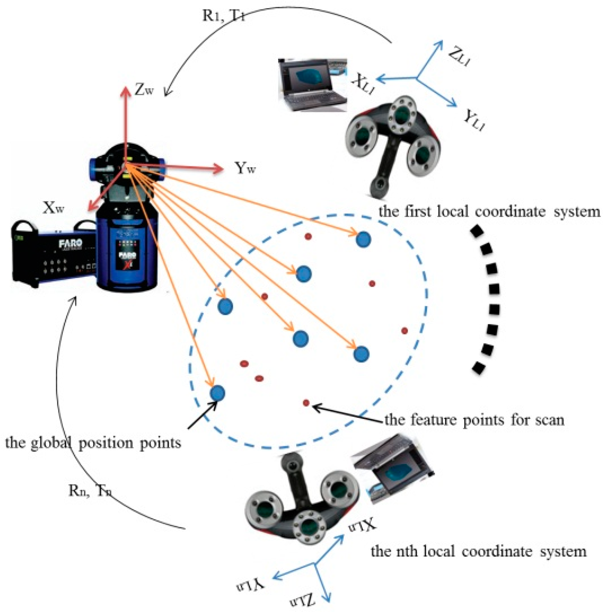
2.2. Multi-Sensor Data Fusion
We assume that the laser tracker’s coordinate system is the global coordinate system, expressed by O-XWYWZW and the coordinate system of MAXscan is the local coordinate system O-XLYLZL. With the movement of MAXscan, the ith local coordinate system is expressed by O-XLiYLiZLi (i = 1, 2, 3 …, n).
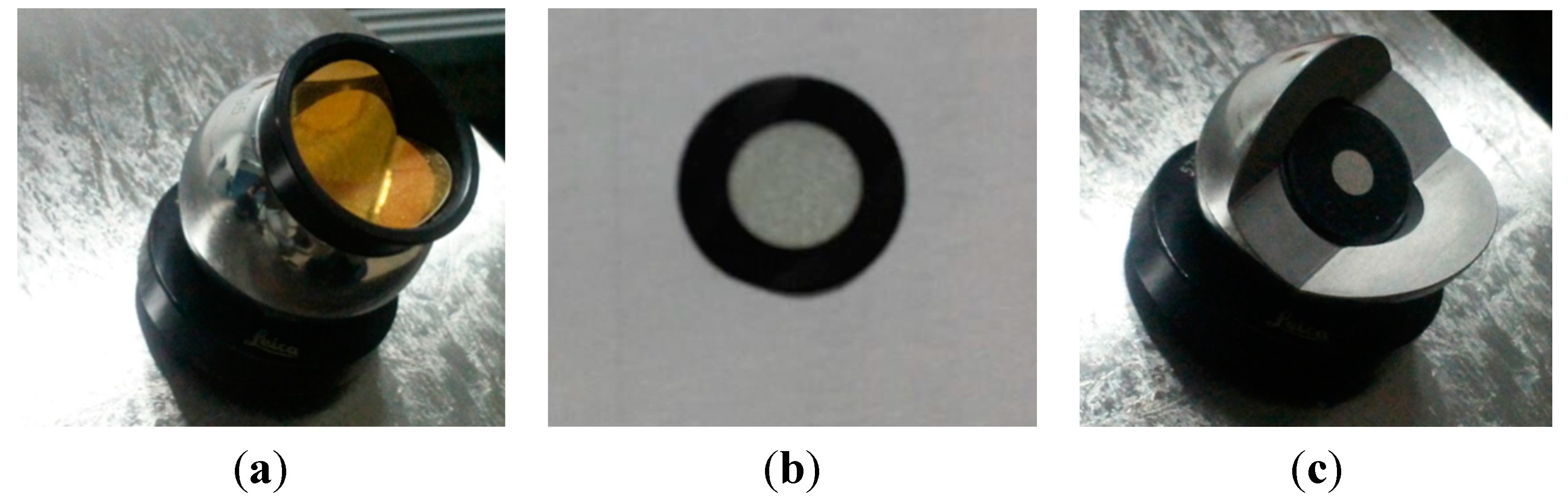
When both the sensors are locked onto the same target, integrating the 3-D measurements from different instruments in a global coordinate system is possible. These targets are the reference global position points. However, both instruments have their own specific targets. Wide-angle retro-reflectors known as Tooling Ball Reflectors (TBRs) are used as the probe of the laser tracker as illustrated in
Figure 4a, whose centers are considered as the global position points. The retro-reflective targets (RRTs), as shown in
Figure 4b, are pasted on the object to facilitate the simultaneous measurement of 3-D surface geometry and estimation of a model of positioning features for tracking, so we must solve the inconsistency. To measure the same physical features, the RRT pasted on the center of the 1.5-inch diameter half-sphere probe tip, which is the commercially available target, is used as shown in
Figure 4c. It provides same centerline value as the TBR and it is used as a medium between laser tracker systems to optical scanning systems.
Figure 4.
(a) TBR for the laser tracker mounted on a nest; (b) RRTs pasted on the object; (c) RRT pasted on the center of a 1.5-inch tip on the nest to assess the same point with the laser tracker and MAXscan.
Figure 4.
(a) TBR for the laser tracker mounted on a nest; (b) RRTs pasted on the object; (c) RRT pasted on the center of a 1.5-inch tip on the nest to assess the same point with the laser tracker and MAXscan.
The coordinate of a point in O-X
WY
WZ
W is noted by ξ
W = [X
W Y
W Z
W] and that in O-X
LiY
LiZ
Li is ξ
L = [X
L Y
L Z
L]. The spatial relationship of all the local point clouds relative to the global coordinate system can be achieved by the scale parameter k, the rotation matrix
R and the translation vector
T. The coordinate transformation equation is expressed by:
where R = r(ω)r(φ)r(к) =
, T = [x
T y
T z
T]
T.
There are seven undetermined parameters in the above matrix equations, so at least three pair-wise registration points, which are non-collinear and able to be observed simultaneously by the two sensors, should be measured to calculate the undetermined parameters. In general, when the rotation angle is large, the error generated by the linear model as Equation (1) cannot be neglected, so we estimate these parameters based on the improved Gauss-Newton optimization approach. Compared to the traditional Gauss-Newton optimization approach method, the improved approach is convergent, no matter what the initial value is. Moreover, the computing speed is improved.
Firstly, we suppose that the error of the linear model is expressed by Equation (2):
where f(X) is the nonlinear function vector consisted of the unknown parameter vector X = [x
T y
T z
T ω φ к k]
T.
Based on the traditional solution of the least squares adjustment, the objective function is constructed by:
where
P is weight matrix, and
P = σ
2[Var(V)]
−1, σ
2 is the variance factor of unit weight.
It means to meet the nonlinear equations:
Then, Taylor’s expansion in initial value X = [x
T0 y
T0 z
T0 ω
0 φ
0 к
0 k
0]
T is expressed by:
So:
where
.
Thus the optimal solution is estimated by:
Finally, in this iterative process,
is updated as the initial value until
reaches the threshold value. Threshold value is a tiny number. In this paper, the value is 1 × 10⁻⁵.
Thus, from Equation (7), we can obtain the rotation matrix R and the translation vector T. However, with the existing of the measurement error, R and T are not accurate enough. As the number of the coordinate transformations rises, errors will accumulate. In this paper, we adopt the multi-sensor data fusion proposed by Nandi to improve the accuracy and decrease the transformation error [
19].
For notational ease, M
i (
i = 1, …, n) is the 3-D coordinate from the ith sensor, and n is the number of the sensors. It usually can be expressed by means of a function of θ
i:
where
represents the additive noise.
Equation (9) is deduced by Taylor expanding M
i and neglecting the quadratic term:
where J
i is the Jacobian matrix with respect to θ:
Assuming a Gaussian distribution for
, we get the covariance matrix for the
ith sensor:
where
is the fused result for M
i:
where the weight matrix W
i for the
ith sensor is determined by the covariance matrix V [M
i]:
Then the covariance matrix V[
] is:
Obviously, from Equation (14), we can obtain that V[]−1 > V[Mi]−1. Thus, V[] < V[Mi]. This proves that after the multi-sensor data fusion, the data accuracy is improved.
4. Practical Application
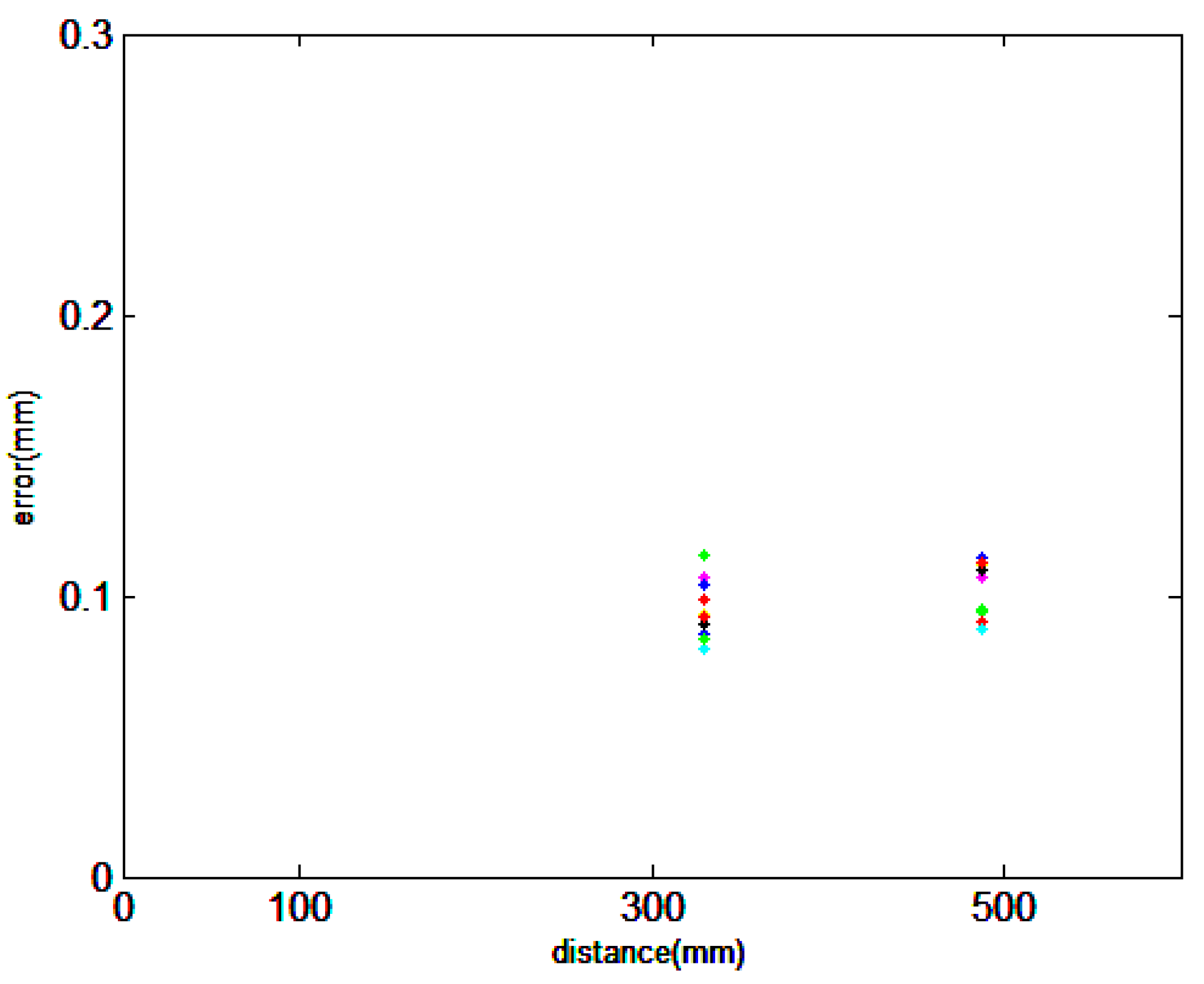
For the purpose of verifying the practicality of the proposed measurement method, a small ring gauge and a large-scale gear rim were chosen as measurement objects. Considering that there is no surface and geometry information to measure the length on the flat concrete wall, we apply this combined method on a ring gauge with the standard length of 500.125 mm, which is measured by the laser tracker, as shown in
Figure 11. Similarly, the length is also measured only by MAXscan and the combined system, respectively. The comparative experiment results are shown in
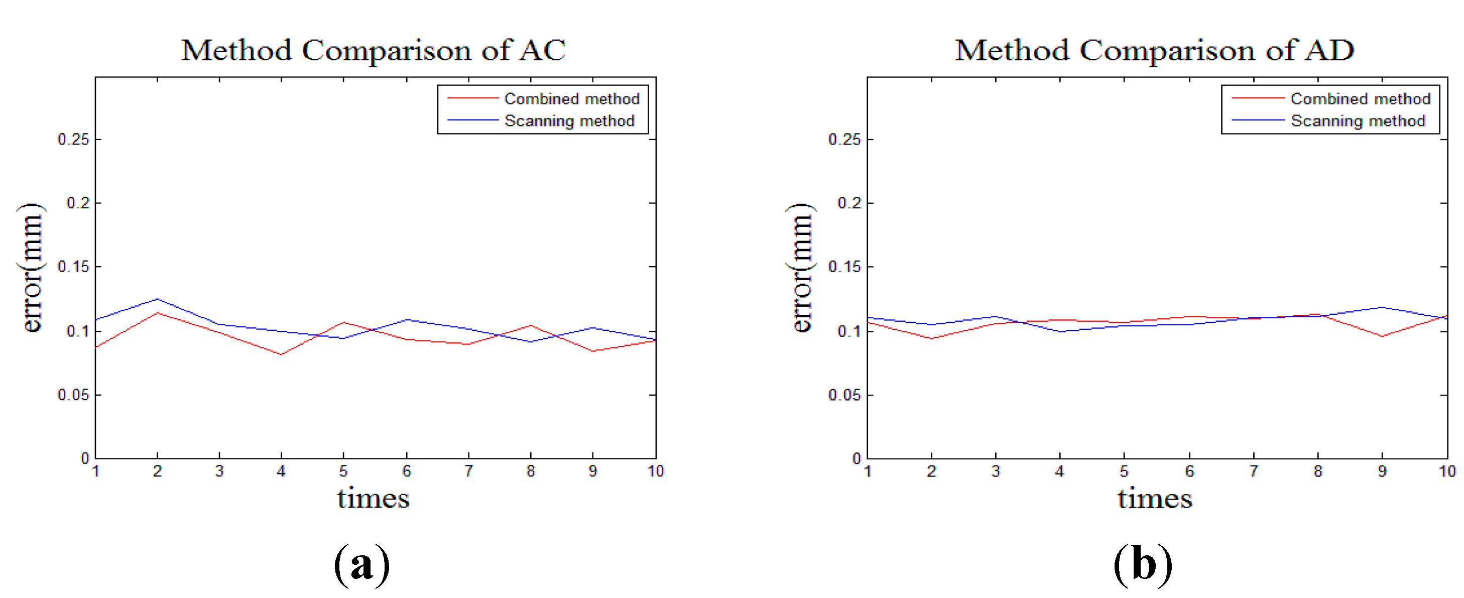
Figure 12. It is observed that the length measured by the combined measurement is closer to the standard. It has been successfully verified that combined measurement effectively reduces the accumulated error caused by a large number of image registration and transformation steps and improves the measurement accuracy.
Figure 11.
The ring gauge with the reference global position points.
Figure 11.
The ring gauge with the reference global position points.
Figure 12.
The results of the deviation comparison.
Figure 12.
The results of the deviation comparison.
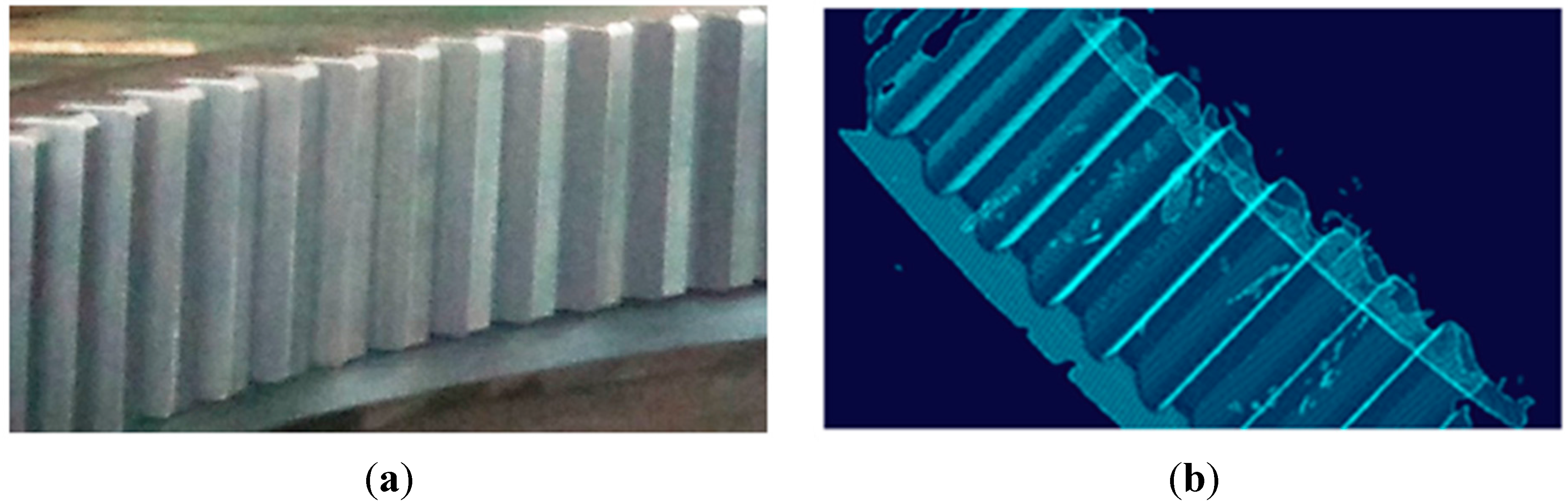
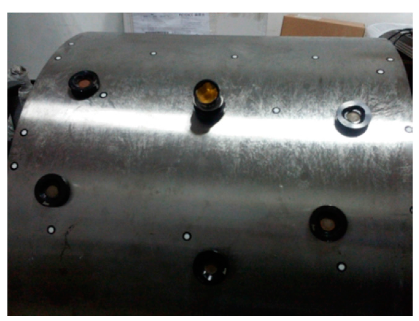
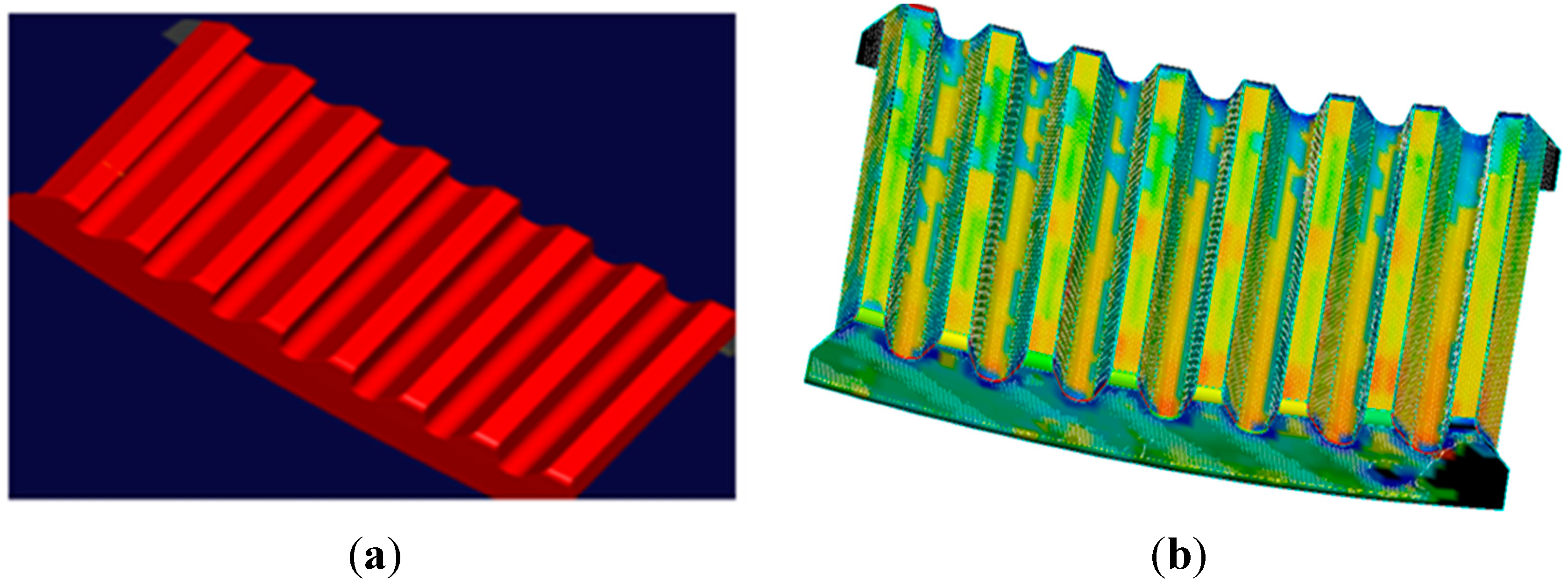
As the ring gauge is small, a large-scale gear rim, as shown in
Figure 13a, is measured by the combined method. The gear rim is widely used as a key mechanical part in power stations, dams, offshore platforms and so on. The measurement accuracy during the fabrication and assembly process has a considerable influence on the performance of products.
Figure 13.
(a) A large-scale gear rim; (b) The original cloud.
Figure 13.
(a) A large-scale gear rim; (b) The original cloud.
The gear rim’s radius is 1163 mm, length about 560 mm and width 220 mm. A total of 66,893 points are acquired by the proposed method, as shown in
Figure 13b. Then, in order to derive the reconstructed model, a high-accuracy 3-D reconstruction method based on NURBS surface is adopted for data processing and surface reconstruction. In the surface reconstruction, NURBS is better able to control the degree of the curve than the traditional grid modeling approaches, such as Bezier, triangle-Bezier or B-spline, and thus it is commonly used to create a high fidelity model. What’s more, many applications involving CAD/CAM, virtual reality, animation and visualization use models described by NURBS surfaces. Over the last few years, they have become very important in industry, and they are used to represent shapes of automobiles, aeroplanes, ships, mechanical parts,
etc. [
20,
21]. Therefore, in this paper, the 3-D solid model is reconstructed based on the NURBS surface, whose mathematical model can be expressed by:
where P
ij (0 ≤
i ≤ n, 0 ≤
j ≤ m) is the control points, ω
ij is corresponding weight of P
ij, N
ik(u) and N
jl(v) are the normalized B-spline base functions of order
k and
l, respectively, defined over vector U = {u
0, u
1, …, u
n, …, u
n+k} and V = {v
0, v
1, …, v
m, …, v
m+k}.
We adopt the commercial software package Imageware to reconstruct the surface. The NURBS parameters can be calculated and determined by the software automatically. As the number of points improves, the reconstructed surface becomes a better approximation of the true shape. With the use of the combined measurement method, big curvature surfaces can be scanned densely to provide abundant information and then reconstructed with high fidelity. Meanwhile, the fitting skills also have an impact on the accuracy. As shown in
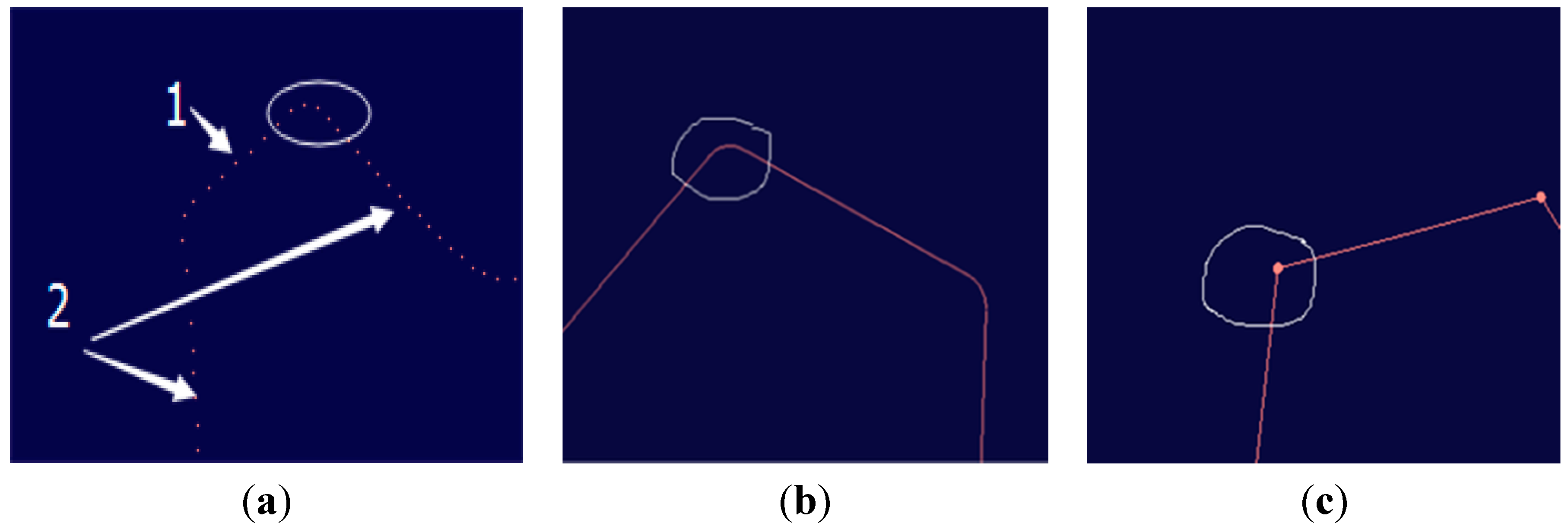
Figure 13, there are fillets on the edge. They are produced by the processing technology to remove burrs, reduce the stress concentration and improve the strength of the gear rim. However, with the existence of the fillets, we cannot extract the structural contours for the gear rim. If the curve is reconstructed just by the software automatically, the reconstruction model will show a round corner as shown in
Figure 14b. In this paper, each tooth of the gear is divided into two parts. Part 1 is the addendum circle and part 2 includes the left and right flank of a tooth, as shown in
Figure 14a. According to the points in the corresponding part, three lines are reconstructed, respectively. Finally, these lines are extended and trimmed in the intersection, as shown in
Figure 14c. This method is not only used in the measurement field, but also applied in practical manufacturing.
Figure 14.
The fitting result comparison: (a) The point data; (b) The conventional method; (c) The proposed method.
Figure 14.
The fitting result comparison: (a) The point data; (b) The conventional method; (c) The proposed method.
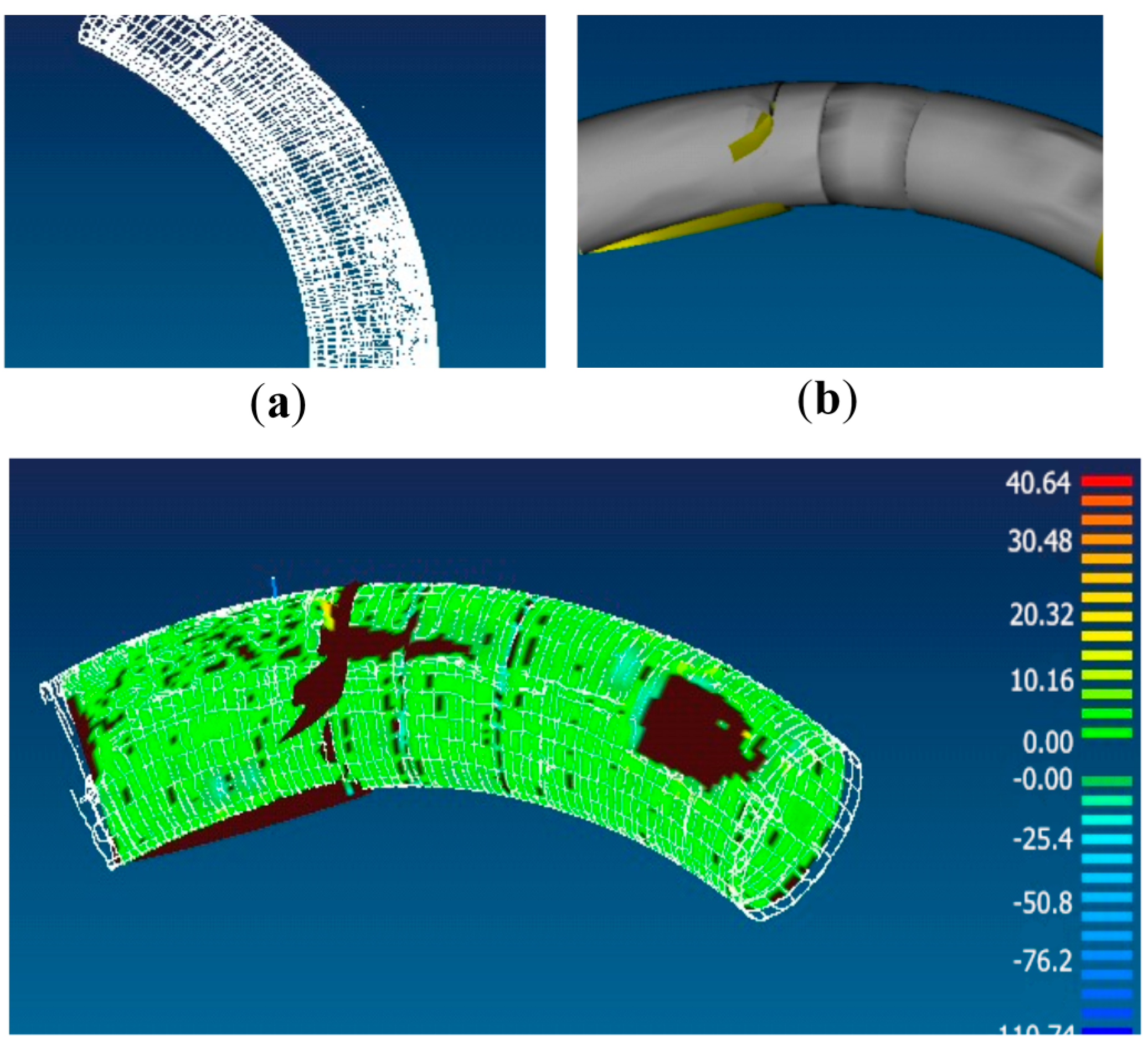
Consequently, the surface model is reconstructed from the point cloud data, as shown in
Figure 15a. Furthermore, the error of the reconstructed surface is analyzed. The analysis results are summarized in
Table 2. The average Euclidean error in the process of establishing the computer 3-D model of the gear rim is 0.0816 mm. The distribution of the error caused by reconstruction is shown in
Figure 15b in which the surface error distribution is in the light yellow band and light blue band, indicating that almost all error is between ±0.1 mm.
Table 2.
The error evaluation of the surface.
Table 2.
The error evaluation of the surface.
| | Mean Error | Max Error | Standard Deviation |
|---|
| Lateral deviation | 0.0000 | 0.0001 | 0.0000 |
| Negative normal deviation | −0.0821 | −0.4300 | 0.0582 |
| Positive normal deviation | 0.0810 | 0.3477 | 0.0704 |
| Euclidean error | 0.0816 | 0.4300 | 0.0647 |
Figure 15.
(a) The fitting surface; (b) Error distribution diagram.
Figure 15.
(a) The fitting surface; (b) Error distribution diagram.
5. Error Analysis and Synthesis
The error analysis and synthesis of the entire system is necessary to guarantee the application of the established system in the industrial field, so the total error model from the measurement entities to the surface model should be established. Error between the measurement entities and the surface model is the cumulative error caused by all aspects of the whole process, which include the measurement error of the laser tracker ∆
W, the measurement error of the handheld laser scanning sensor ∆
S, data processing error Δp, the transformation error ∆
T and the surface reconstruction error ∆
R. Assuming all of the errors meet a normal distribution, the total error may be considered as:
The data processing error Δp refers to errors generated from smoothing of noisy data and streamlining of redundant data. Due to only eliminating the obvious noise point of a large area manually during the data processing without smoothing and streamlining, the data processing errors are negligible. After the multi-sensor data fusion, the transformation error is decreased and can be also ignored relative to the measurement error of the laser tracker and the handheld laser scanning sensor [
22,
23]. The maximum length of the workpiece is 560 mm, and thus the measurement error is:
Meanwhile, as the average Euclidean error is the synthesized error of the surface reconstruction process, the surface reconstruction error ∆R of the gear rim is 0.0816 mm. Thus, according to the Equation (16), the total error is 0.0963 mm.


