
A Survey of Wireless Sensor Network Based Air Pollution Monitoring Systems

 ,
,
Abstract
:1. Introduction

| City | Number of Stationary Monitors | Coverage Area | Coverage Per Monitor (Number of Football Fields) |
|---|---|---|---|
| Beijing, China | 35 [7] | 16,000 km2 | 64,025 |
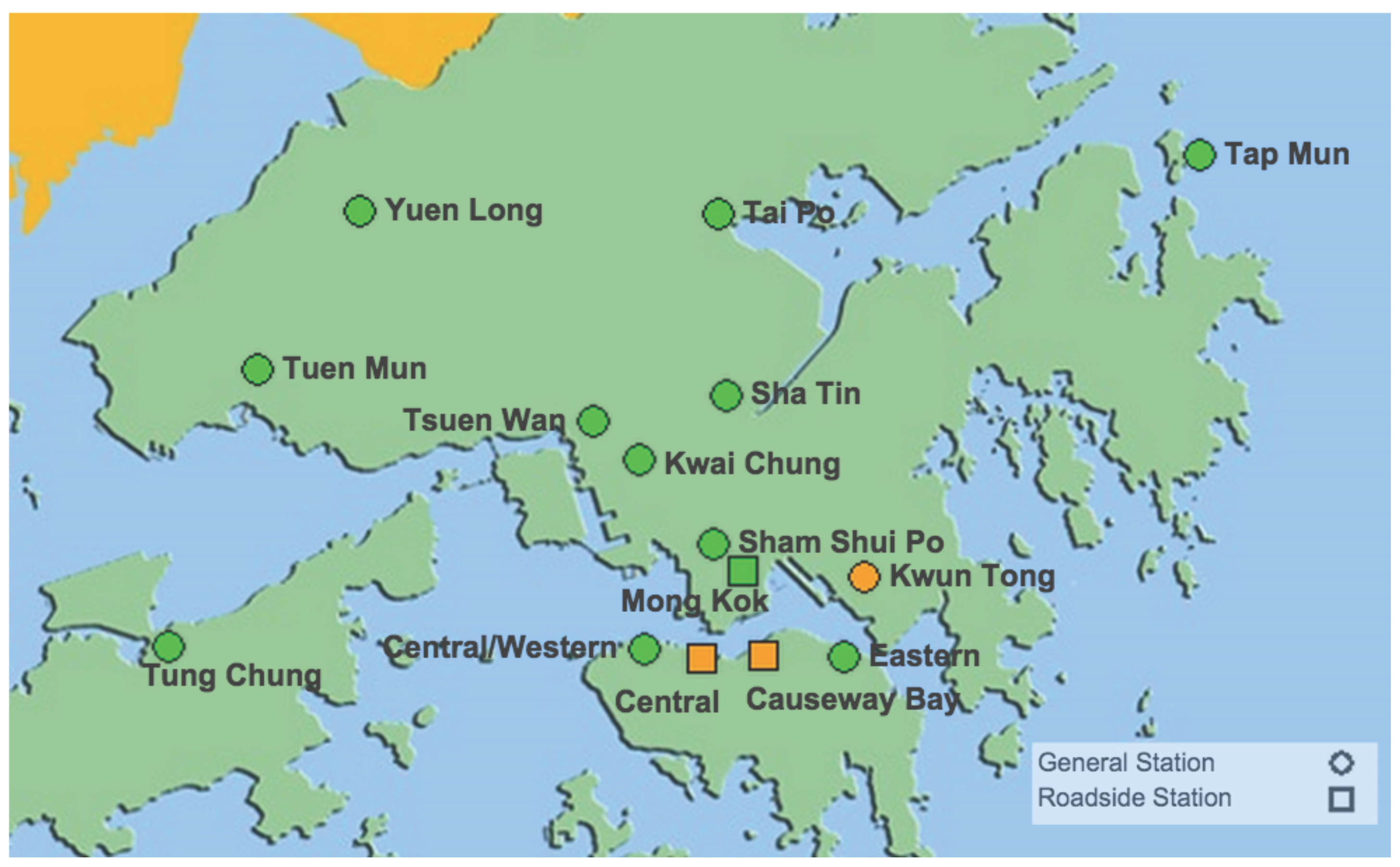
| Hong Kong, China | 15 [6] | 2700 km2 | 25,210 |
| New York, USA | 44 [8] | 1200 km2 | 3820 |
| London, UK | 123 [9] | 1600 km2 | 1822 |
2. Air Quality Standards
| Pollutant | Health Effects |
|---|---|
| Carbon Monoxide (CO) | Reducing oxygen capacity of the blood cells leadsto reducing oxygen delivery to the body’s organsand tissues. Extremely high level can cause death. |
| Nitrogen Dioxide (NO2) | High risk factor of emphysema, asthma andbronchitis diseases. Aggravate existing heartdisease and increase premature death. |
| Ozone (O3) | Trigger chest pain, coughing, throat irritationand congestion. Worsen bronchitis, emphysemaand asthma. |
| Sulfur Dioxide (SO2) | High risk factor of bronchoconstrictionand increase asthma symptoms. |
| Particulate Matter (PM2.5 & PM10) | Cause premature death in people with heart andlung diseases. Aggravate asthma, decrease lungfunction and increase respiratory symptomslike coughing and difficulty breathing. |
| Lead (Pb) | Accumulate in bones and affect nervous system,kidney function, immune system, reproductivesystems, developmental systems and cardiovascularsystem. Affect oxygen capacity of blood cells. |
| Pollutant | EPA [37] | WHO [38,39,40] | EC [41] | MEP [42] | EPD [43] | |
|---|---|---|---|---|---|---|
| Carbon Monoxide (CO) | 9 ppm (8 h) 35 ppm (1 h) | 100 mg/m3 (15 min) 15 mg/m3 (1 h) 10 mg/m3 (8 h) 7 mg/m3 (24 h) | 10 mg/m3 (8 h) | 10 mg/m3 (1 h) 4 mg/m3 (24 h) | 30 mg/m3 (1 h) 10 mg/m3 (8 h) | |
| Nitrogen Dioxide (NO2) | 100 ppb (1 h) 53 ppb (1 year) | 200 μg/m3 (1 h) 40 μg/m3 (1 year) | 200 μg/m3 (1 h) 40 μg/m3 (1 year) | 200 μg/m3 (1 h) 80 μg/m3 (24 h) 40 μg/m3 (1 year) | 200 μg/m3 (1 h) 40 μg/m3 (1 year) | |
| Ozone (O3) | 75 ppb (8 h) | 100 μg/m3 (8 h) | 120 μg/m3 (8 h) | 200 μg/m3 (1 h) 160 μg/m3 (8 h) | 160 μg/m3 (8 h) | |
| Sulfur Dioxide (SO2) | 75 ppb (1 h) 0.5 ppm (3 h) | 500 μg/m3 (10 min) 20 μg/m3 (24 h) | 350 μg/m3 (1 h) 125 μg/m3 (24 h) | 500 μ g/m3 (1 h) 150 μg/m3 (24 h) 60 μg/m3 (1 year) | 500 μg/m3 (10 min) 125 μg/m3 (24 h) | |
| Particulate Matter | PM2.5 | 35 μg/m3 (24 h) 12 μg/m3 (1 year) | 25 μg/m3 (24 h) 10 μg/m3 (1 year) | 25 μg/m3 (1 year) | 75 μg/m3 (24 h) 35 μg/m3 (1 year) | 75 μg/m3 (24 h) 35 μg/m3 (1 year) |
| PM10 | 150 μg/m3 (24 h) | 50 μg/m3 (24 h) 20 μg/m3 (1 year) | 50 μg/m3 (24 h) 40 μg/m3 (1 year) | 150 μg/m3 (24 h) 70 μg/m3 (1 year) | 100 μg/m3 (24 h) 50 μg/m3 (1 year) | |
| Lead (Pb) | 0.15 μg/m3 (3 month) | 0.5 μg/m3 (1 year) | 0.5 μg/m3 (1 year) | 1 μg/m3 (3 month) 0.5 μg/m3 (1 year) | 1 μg/m3 (3 month) 0.5 μg/m3 (1 year) | |
| Health Risk Category | AQHI |
|---|---|
| Low (Green) | 1 |
| 2 | |
| 3 | |
| Moderate (Orange) | 4 |
| 5 | |
| 6 | |
| High (Red) | 7 |
| Very High (Brown) | 8 |
| 9 | |
| 10 | |
| Serious (Black) | 10+ |
3. Air Pollution Monitoring Equipment
| Pollutant | Example Product | Measurement Method | Resolution | Accuracy | Range | Price (USD) | |
|---|---|---|---|---|---|---|---|
| PM2.5 | Met One Instrument BAM-1020 Beta Attenuation Monitor [56] | Beta Attenuation | 1 μg/m3 | ±1 μg/m3 | 0–1000 μg/m3 | About $25,000 | |
| Met One Instrument Aerocet 831 Aerosol Mass Monitor [57] | Light Scatting | 0.1 μg/m3 | ±10% of reading | 0–1000 μg/m3 | About $2000 | ||
| Alphasense OPC-N2 Particle Monitor [58] | Light Scatting | Not Provided | Not Provided | Not Provided | About $500 | ||
| Sharp Microelectronics DN7C3CA006 PM2.5 Module [59] | Light Obscuration (Nephelometer) | Not Provided | Not Provided | 25–500 μg/m3 | About $20 | ||
| PM10 | Teledyne Model 602 BetaPLUS Particle Measurement System [60] | Beta Attenuation | 0.1 μg/m3 | ±1 μg/m3 | 0–1500 μg/m3 | About $30,000 | |
| Met One Instrument Aerocet 831 Aerosol Mass Monitor [57] | Light Scatting | 0.1 μg/m3 | ±10% of reading | 0–1000 μg/m3 | About $2000 | ||
| Alphasense OPC-N2 Particle Monitor [58] | Light Scatting | Not Provided | Not Provided | Not Provided | About $500 | ||
| Sharp GP2Y1010AU Air Quality Sensor [61] | Light Obscuration (Nephelometer) | Not Provided | Not Provided | 0–500 μg/m3 | About $20 | ||
| Lead (Pb) | Operation in Lab | - | - | - | - | - | |
| Pollutant | Example Product | Measurement Method | Resolution | Accuracy | Range | Price (USD) | |
|---|---|---|---|---|---|---|---|
| Carbon Monoxide (CO) | Teledyne Model T300U Gas Filter Correlation Carbon Monoxide Analyzer [62] | IR Absorption with Gas Filter Correlation Wheel | 0.1 ppb | ±0.5% of reading | 0–100 ppb or 0–100 ppm | About $30,000 | |
| Aeroqual Series 500 with CO Sensor Head [63] | Electrochemical Sensor | 10 ppb | ±0.5 ppm at 0–5 ppm or ±10% at 5–25 ppm | 0–25 ppm | About $2000 | ||
| Alphasense B4 Series CO Sensor [64] | Electrochemical Sensor | 4 ppb | Not Provided | 0–1000 ppm | About $200 | ||
| Hanwei MQ-7 CO Sensor [65] | Solid-State Sensor | Not Provided | Not Provided | 20–2000 ppm | About $10 | ||
| Nitrogen Dioxide (NO2) | Teledyne Model T500U Nitrogen Dioxide Analyzer [66] | Cavity Attenuated Phase Shift Spectroscopy | 0.1 ppb | ±0.5% of reading | 0–5 ppb or 0–1 ppm | About $30,000 | |
| Aeroqual Series 500 with NO2 Sensor Head [67] | Electrochemical Sensor | 1 ppb | ±0.02 ppm at 0–0.2 ppm or ±10% at 0.2–1 ppm | 0–1 ppm | About $2000 | ||
| Alphasense B4 Series NO2 Sensor [68] | Electrochemical Sensor | 12 ppb | Not Provided | 0–20 ppm | About $200 | ||
| SGXSensorTech MiCS-2714 NO2 Sensor [69] | Solid-State Sensor | Not Provided | Not Provided | 0.05–10 ppm | About $10 | ||
| Ozone (O3) | Teledyne Model 265E Chemiluminescence Ozone Analyzer [70] | Chemiluminescence Detection | 0.1 ppb | ±0.5% of reading | 0–100 ppb or 0–2 ppm | About $25,000 | |
| Aeroqual Series 500 with O3 Sensor Head [71] | Solid-State Sensor | 1 ppb | ±5 ppb | 0–150 ppb | About $2000 | ||
| Alphasense B4 Series O3 Sensor [72] | Electrochemical Sensor | 4 ppb | Not Provided | 0–5 ppm | About $200 | ||
| Hanwei MQ-131 O3 Sensor [73] | Solid-State Sensor | Not Provided | Not Provided | 10–1000 ppm | About $10 | ||
| Sulfur Dioxide (SO2) | Teledyne Model 6400T/6400E Sulfur Dioxide Analyzer [74] | UV Fluorescence | 0.1 ppb | ±0.5% of reading | 0–50 ppb or 0–20 ppm | About $30,000 | |
| Aeroqual Series 500 with SO2 Sensor Head [75] | Electrochemical Sensor | 10 ppb | ±0.05 ppm at 0–0.5 ppm or ±10% at 0.5–10 ppm | 0–10 ppm | About $2000 | ||
| Alphasense B4 Series SO2 Sensor [76] | Electrochemical Sensor | 5 ppb | Not Provided | 0–100 ppm | About $200 | ||
| Hanwei MQ-136 SO2 Sensor [77] | Solid-State Sensor | Not Provided | Not Provided | 0–200 ppm | About $50 | ||
| Sensor Type | Detectable Gases | Linearity | Cross Sensitivity | Power Consumption | Maintenance | Response Time (T90) | Life Expectancy |
|---|---|---|---|---|---|---|---|
| Electro-chemical [78] | Gases which are electrochemically active, about 20 gases | Linear at room temperature | Can be eliminated by using chemical filter | Lowest, very little power consumption | Low | <50 s | 1–2 years |
| Catalytic [79] | Combustible gases | Linear at 400 °C to 600 °C | No meaning when measuring mixed gases | Large, need to heat up to 400 °C to 600 °C | Lose sensitivity with time due to poisoning and burning out | <15 s | Up to 3 years |
| Solid-state [80] | About 150 different gases | Linear at operational temperature | Can be minimized by using appropriate filter | Large, need heating element to regulate temperature | Low | 20 s to 90 s | 10+ years |
| Non-dispersive Infrared [81] | Hydrocarbon gases and carbon dioxide | Nonlinear, need linearize procedure | All hydrocarbons share a similar absorption band, make them all cross sensitive | Small, mainly consume by the infrared source | The least | <20 s | 3–5 years |
| Photo-ionization [82] | Volatile organic compounds (VOCs) | Relatively linear | Any VOCs with ionization potent- ials less than the ionizing potential of the lamp used will be measured | Medium, mainly consume by the ultraviolet source | The lamp requires frequent cleaning | <3 s | Depend on the Ultraviolet lamp, normally 6000 h |
3.1. Gas Sensor
- CO: Can be well detected by solid-state and electrochemical sensors.
- NO2: Can be well detected by solid-state and electrochemical sensors. Need to consider the interference gas O3. Proper methods can be applied to reduce the interference.
- O3: Can be well detected by solid-state and electrochemical sensors. Need to consider the interference gas NO2. Proper methods can be applied to reduce the interference.
- SO2: Can only be well detected by solid-state and electrochemical sensors. It poisons the catalytic sensors. The sensitivity of NDIR sensors is not high enough.
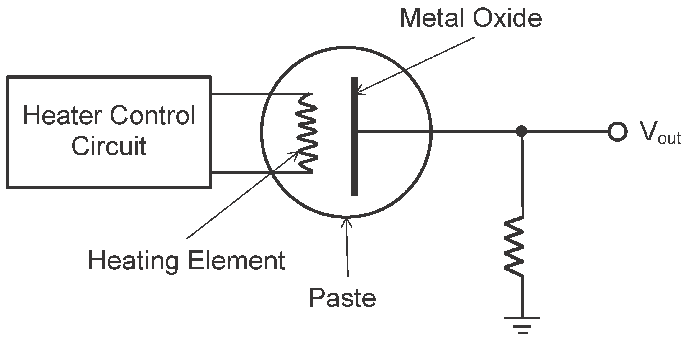
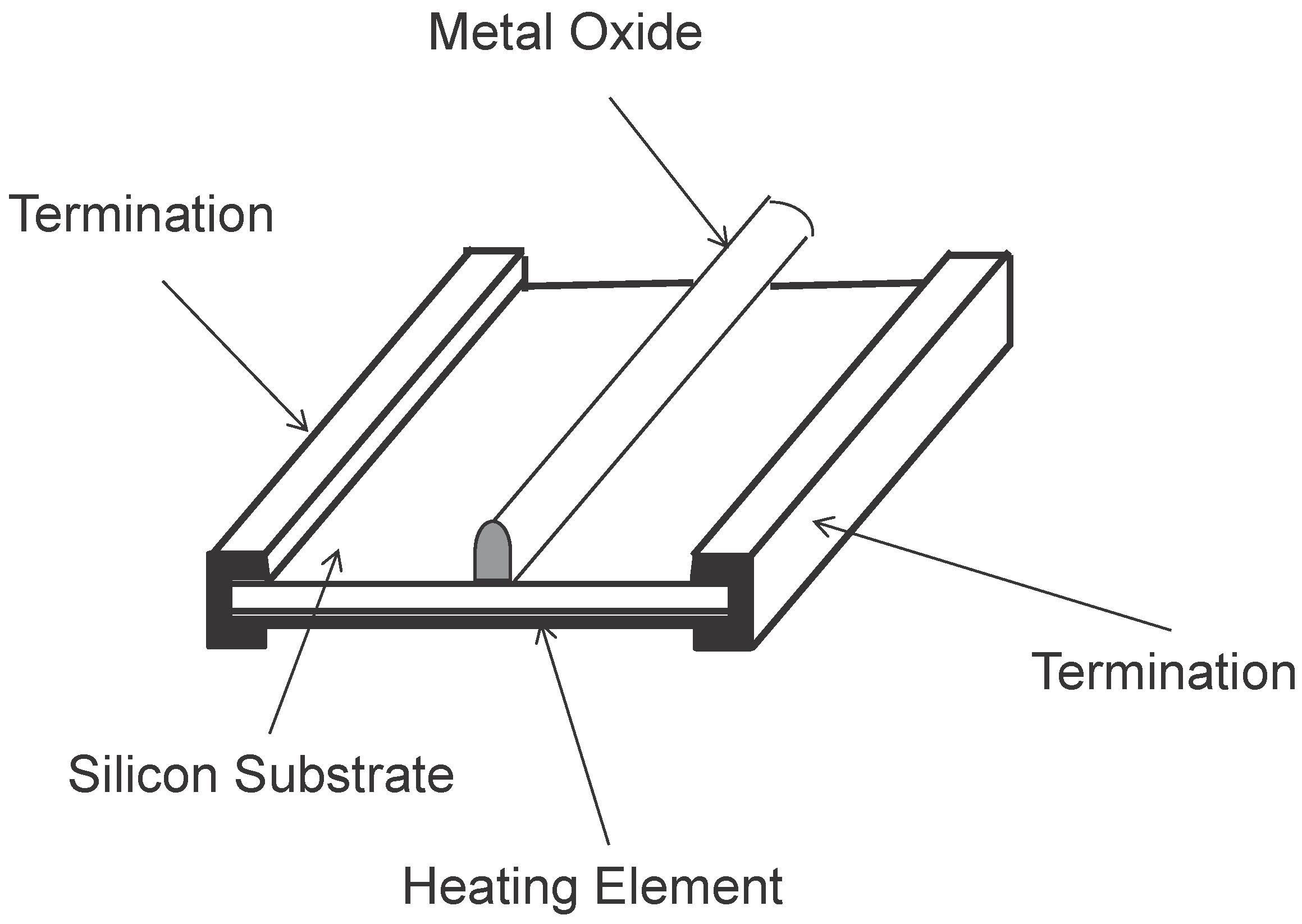
3.1.1. Solid-state Gas Sensor [80]
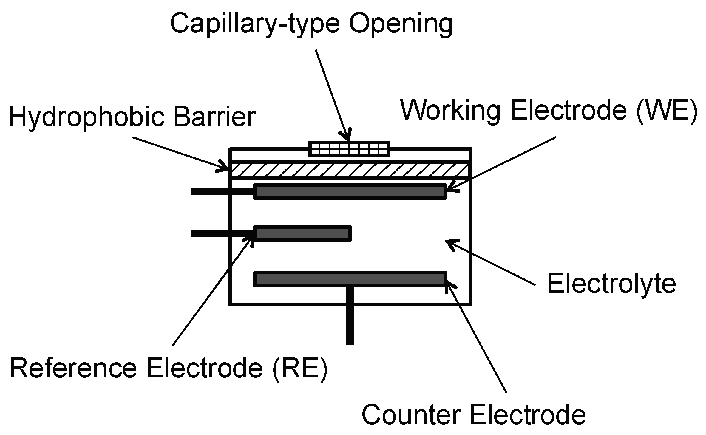
3.1.2. Electrochemical Gas Sensor [78]
3.2. Particulate Matter Sensor
3.2.1. Tapered Element Oscillating Micro-Balance (TEOM) Analyzers [88]
3.2.2. β-Attenuation Analyzers [89]
3.2.3. Black Smoke Method [90]
3.2.4. Optical Analyzers [91]
- Light Scatting:This category of optical analyzers uses a high-energy laser as the light source. When a particle passes through the detection chamber that only allows single particle sampling, the laser light is scattered by the particle. A photo detector detects the scatting light. By analyzing the intensity of the scatting light, researchers can deduce the size of the particle. Also, the number of particle counts can be deduced by counting the number of detecting light on the photo detector (see Figure 5). The advantage of this approach is that a single analyzer can detect particles with different diameters simultaneously (i.e., PM2.5, PM5 and PM10). However, the particle counts need to be converted to mass concentration by calculation (depends on the particle counts, particle types and particle shapes) and this will introduce errors that further affect the precision and accuracy of the analyzers.
- Direct Imaging:In a direct imaging particle analyzer, a beam of halogen light illuminates the particles and the shadow of each particle is projected to a high definition, high magnification and high resolution camera. The camera records the passing particles. The video is then analyzed by computer software to measure the PM’s attributes. Both size and counts of the PMs in the ambient air can be obtained. What’s more, the color and the shape of the particles can also be detected.
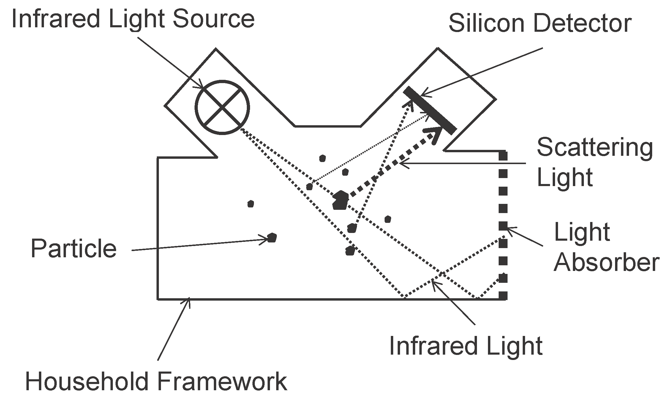
- Light Obscuration (Nephelometer):This category of optical analyzers uses the fastest particle concentration (μg/m3) measurement method with high precision and low detection limited. A nephelometer is an instrument that measures the size and mass concentration of PM in the ambient air. In a nephelometer, a near infrared LED is used as the light source and a silicon detector is used to measure the total light scattered (which is majorly responsible for the total light extinction) by the PMs (see Figure 6). By analyzing the intensities (in magnitude) of the scattered light and the shape of the scattering pattern, both the size distribution and the mass concentration can be determined right away [92].

| Measurement Method | Advantages | Disadvantages | Accuracy |
|---|---|---|---|
| Tapered Element Oscillating Microbalance (TEOM) analyzers | Provide real time (<1 h) data with high precision. | A heater must be used which leads to lose of semi-volatile material. Usually with large size, heavy weight and high cost. | ±0.5 μg/m3 |
| β-attenuation analyzers (BAM) | Provide real time (<1 h) data with high precision. | A radioactive source is used. If heater is used some semi-volatile material may be lost. Need to replace the paper filter periodically. Usually with large size, heavy weight and high cost. | ±1.0 μg/m3 |
| Black smoke method | Simple, robust and inexpensive. Easy to maintain. Short sample time (in minutes). | Measure the darkness rather than the mass concentration of the particulate matters. Darkness-mass factor may change from time to time and location to location. | ±2.0 μg/m3, or higher |
| Optical analyzers | Small, light weight and usually battery operated. Short sample time (in seconds or minutes). Can measure different sizes of particles simultaneously. | Depends on some assumptions of particle characteristics (e.g. each particle is perfect bean-like shape). These assumptions may be different from time to time and location to location. | Depends on the analyzer type and usually not specifically declared by the manufacture. |
4. State-of-The-Art WSN Based Air Pollution Monitoring Systems

4.1. Static Sensor Network (SSN)
- Loose constraint on energy consumption (The sensor nodes are typically powered by batteries with large capacity or energy harvest devices or power line.)
- No locating device (The location of a sensor node is known once it was deployed since the sensor node is stationary.)
- Loose limitations on weight and size (The carrier of the sensor node is able to carry sufficient enough weight.)
- Multiple sensors per node (One sensor node can equip with several types of sensors because of the loose limitations on weight and size.)
- Accurate and reliable data (Sensor node can integrate with assisting tools because of the loose limitations on weight and size.)
- Guaranteed network connectivity (Once the stationary sensor node joined the network, the topology is fixed and the connectivity is guaranteed.)
- Well calibrated and maintained sensors (The sensor nodes can be well calibrated and maintained by the professionals periodically.)
- Careful placement of sensor nodes requirement (This is because of the location dependence of air pollutants.)
- Large number of sensor nodes requirement (Data with sufficient geographic coverage and spatial resolution are only achievable by increasing the number of the stationary sensor nodes.)
- Resource wasting in certain level (The stationary sensor nodes are in sleep mode most of the time because continuously updating data at one location is pointless [13].)
- Inconveniences of calibration and maintenance (The professionals need to visit all stationary sensor nodes, which is a time and manpower consuming task, to perform operations.)
- 2-Dimensional data acquisition (Only the air quality of urban surface is monitored.)
- Customized network requirement (A customized wireless or wired network is required when the cellular network is not utilized.)
4.2. Community Sensor Network (CSN)
- Cost efficiency (The sensor node utilizes the cellphone’s GPS module and the cellular network, or even the cellphone’s computational power.)
- Coupled data generators and consumers (Local or personal air pollution information is available.)
- Public-driven property (The cost of the sensor nodes and the data transmission can be apportioned by the users. It is costly and infeasible for a single agency to acquire all the sensor nodes.)
- Automatic gathering property (The sensor nodes are densely distributed at locations with gathering people automatically. Data with higher spatial resolution and accuracy are achievable in such case.)
- Mobility of sensor nodes (The mobility of the cellphones or users enlarges the sensor node’s geographic coverage.)
- Public behaviors acquisition ability (Information such as the public movement patterns, and interaction between air quality and public behaviors, is achievable.)
- Low data accuracy and reliability (The sensor nodes are typically put in pockets or handbags. Also, the users spend significant amount of time indoor or inside cars [114]).
- Privacy issues (The users may not want to make their location information public for privacy issues).
- Badly calibrated and maintained sensors (Professional calibrations of sensors performed by the public users are very unlikely. Frequent collections and calibrations of sensors by the professionals are infeasible).
- Serious constraint on energy consumption (The sensor nodes is typically powered by cellphone’s battery or battery with small capacity).
- Uncontrolled or semi-controlled mobility (The routes of the sensor nodes or users are pre-determined. The sensor nodes may squeeze into a small place with crowded people and cause redundant sampling. Some locations may never be visited).
- 2-Dimensional data acquisition (Only the air quality of urban surface is monitored).
- Serious limitations on weight and size (The sensor node should be portable, which affects the accuracy, reliability and number of sensors equipped, because it is carried by user).
4.3. Vehicle Sensor Network (VSN)

- Loose constraint on energy consumption (The sensor nodes are powered by the vehicles’ batteries.)
- Loose limitations on weight and size (The carrier of the sensor node is able to carry sufficient enough weight.)
- Multiple sensors per node (One sensor node can equip with several types of sensors because of the loose limitations on weight and size.)
- Accurate and reliable data (Sensor node can integrate with assisting tools because of the loose limitations on weight and size.)
- High mobility of sensor nodes (The highly mobile vehicles significantly enlarge the sensor node’s geographic coverage.)
- Feasibility in maintenance (The vehicles mounted with sensor nodes can be driven to a specific location. Professionals can perform maintenance on large amount of sensor nodes simultaneously.)
- Well calibrated and maintained sensors (This is because of the feasibility in maintenance of the VSN systems.)
- Automatic gathering property (The sensor nodes are densely distributed at locations with gathering public transportations automatically. Data with higher spatial resolution and accuracy are achievable in such case.)
- Uncontrolled or semi-controlled mobility (The routes of the sensor nodes or public transportations are pre-determined. The sensor nodes may squeeze into a small place with crowded transportations and cause redundant sampling. Some locations may never be visited.)
- Redundant sampling issues (The vehicles may be trapped into traffic jams or parked in parking lots that cause redundant sampling. This issue compromises the spatial and temporal resolutions.)
- Cost inefficiency on carriers (The specially equipped cars may cost a huge amount of money.)
- Locating and communication devices requirement (The system requires GPS modules, and wireless modules or cellular modules.)
- Customized network requirement (A customized wireless network is required when the cellular network is not utilized. The network connectivity may not be guaranteed due to the mobility of vehicles.)
- 2-Dimensional data acquisition (Only the air quality of urban surface is monitored.)
- Spatial-to-Temporal resolution trade-off (Higher spatial coverage at the expense of lower temporal resolution [99].)
| Sensor Network Type | System | Carrier | WSN Type | Sensor Type | Power Source | Locating Device | Computational Power of Sensor Node (Clock Speed/SRAM/Storage) |
|---|---|---|---|---|---|---|---|
| SSN | In [105] | Not mentioned | ZigBee | Electrochemical (O3, CO, NO2) | Not mentioned | None | Arduino (14 MHz/512 KB/2 GB) |
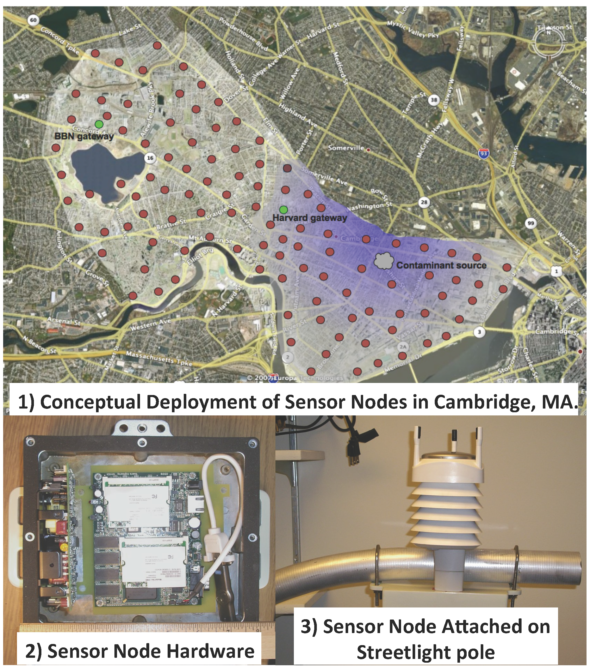
| In [101] | Streetlight pole | Wi-Fi (802.11 a/b/g) | Solid-state (CO2, NO, O3) | Power line | None | Linux based embedded PC (266 MHz/128 MB/1 GB) | |
| In [104] | Not mentioned | Not mentioned | Not mentioned | Not mentioned | Not mentioned | Not mentioned | |
| In [102] | Streetlight pole | ZigBee + Cellular network (GSM) | Solid-state (CO) | Battery | None | Octopus II (1 MHz/10 KB/1 MB) | |
| In [108] | Wall | Wi-Fi (802.11 b/g) | Solid-state (CO, VOCs) | Not mentioned | None | IPu8930 (*/*/512KB) | |
| In [107] | Wall | ZigBee | Solid-state (CO, VOCs) | Battery | None | JN5168 (32MIPs/128KB/*) | |
| In [103] | Station | Cellular network (GPRS) | Solid-state (CO, NO2, O3, H2S) | Battery, Solar panel | None | Arduino (16 MHz/8 KB/2 GB) | |
| CSN | In [10] | Public user | Cellular network | Solid-state (O3) | Battery | Cellphone GPS module | HTC HERO saxophone |
| In [111] | Public user | Not mentioned | Not mentioned | Cellphone battery | Cellphone GPS module | LG VX980 smart phone | |
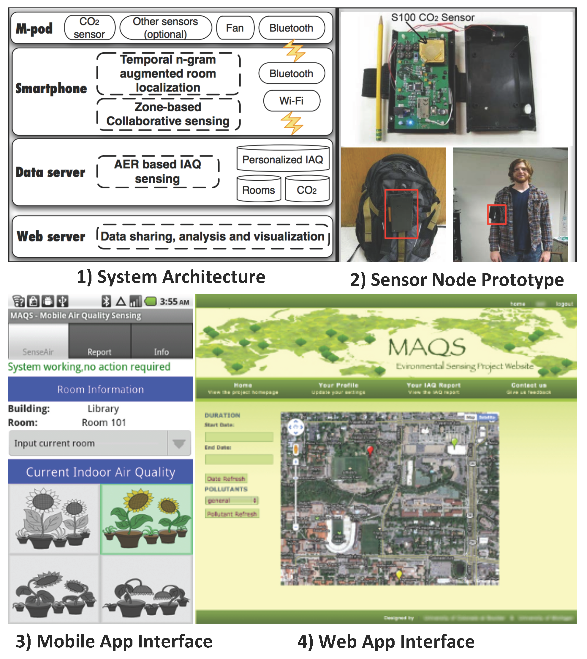
| In [109] | Public user | Wi-Fi | NDIR (CO2), Solid-state (CO, O3) | Battery | Cellphone Wi-Fi module | Arduino (16 MHz/2 KB/32 KB) | |
| In [112] | Public user | Cellular network | Microphone | Cellphone battery | Cellphone GPS module | NOKIA N95 cellphone | |
| In [97] | Public user | Cellular network | Solid-state (CO2, VOCs), Catalytic (H2), Electrochemical (CO) | Battery | Cellphone GPS module | PRO200 Sanyo cellphone | |
| In [113] | Public user | Cellular network | QTF (VOCs) | Battery | Cellphone GPS module | Motorola Q phone | |
| VSN | In [115] | Public transportation | ZigBee | Solid-state (CO, NO2, O3, CO2) | Bus battery | GPS module | Arduino (16 MHz/8 KB/*) |
| In [11] | Car | Wi-Fi | Solid-state (CO, NO2, O3) | Battery | GPS module | 8051 uC (*/4KB/2MB) | |
| In [98] | Car | Cellular network (GSM) | NDIR (CO2) | Car battery | GPS module | JN5139 (16 MHz/96 KB/192 KB) | |
| In [117] | Car | Cellular network | Solid-state (CO), Optical analyzer (PM) | Bus battery | GPS module | Arduino (16 MHz/8 KB/128 KB) | |
| In [118] | Bus | Cellular network (GPRS) | Electrochemical (CO, SO2, NO2) | Not mentioned | GPS module | HCS12/9S12 (25 MHz/12 KB/512 KB) | |
| In [19] | Public transportation | Wi-Fi or ZigBee or Others | DUVAS (O3, NO, NO2, SO2, VOCs) | Not mentioned | Not mentioned | Not mentioned | |
| In [99] | Car | Wi-Fi or Cellular network (GPRS) | Optical analyzer (PM), Solid-state (CO, NO2, NO, VOCs) | Not mentioned | GPS module | Renesas H8S (*/*/*) |
| Sensor Network Type | System | Operation Environment | Sensing Periodic | Number of Sensor Node in System | Geographic Coverage | Data Availability |
|---|---|---|---|---|---|---|
| SSN | In [105] | Outdoor roadside | 200 to 300 s | 60 to 200 | 500 m× 500 m | Email, SMS, Web App |
| In [101] | Outdoor | Not mentioned | about 100 | Harvard campus | Web App | |
| In [104] | Outdoor | Not mentioned | 300 to 1200 | Port Louis | Not mentioned | |
| In [102] | Outdoor roadside | 10 min | 9 | Intersection circle of Keelung Road and Roosevelt Road | Researcher only | |
| In [108] | Indoor | 5 to 60 s | Not mentioned | One floor of a building | Web page | |
| In [107] | Indoor | Adaptive | 36 | One floor of a building | None | |
| In [103] | Outdoor | 1 min | 4 | 1 Km | Web App, mobile App | |
| CNN | In [10] | Outdoor roadside | 5 s | Not mentioned | Citywide | Web App, mobile App |
| In [111] | Outdoor | Not mentioned | Not mentioned | Not mentioned | Not mentioned | |
| In [109] | Indoor | 6 s | Not mentioned | One floor of a building | Web App, mobile App | |
| In [112] | Outdoor | 1 s | Not mentioned | Citywide | Web page, mobile App | |
| In [97] | Outdoor | Not mentioned | Not mentioned | Not mentioned | Web App, mobile App | |
| In [113] | Outdoor | Not mentioned | Not mentioned | Not mentioned | Web App, mobile App | |
| VSN | In [115] | Outdoor roadside | Not mentioned | 1 | Not mentioned | None |
| In [11] | Outdoor roadside | 1 min or few times per hour | Not mentioned | Citywide | Web App | |
| In [98] | Outdoor roadside | 3 s | 16 | National Chiao-Tung University campus | Web App | |
| In [117] | Outdoor roadside | 5 s | 2 | Citywide | Web App | |
| In [118] | Outdoor roadside | Not mentioned | 1 | American University of Sharjah campus | Web App | |
| In [19] | Outdoor roadside | 1 min | 18 | Not mentioned | None | |
| In [99] | Outdoor roadside | Not mentioned | 1 | Nanyang Technological University and neighboring industrial estate | Web App |
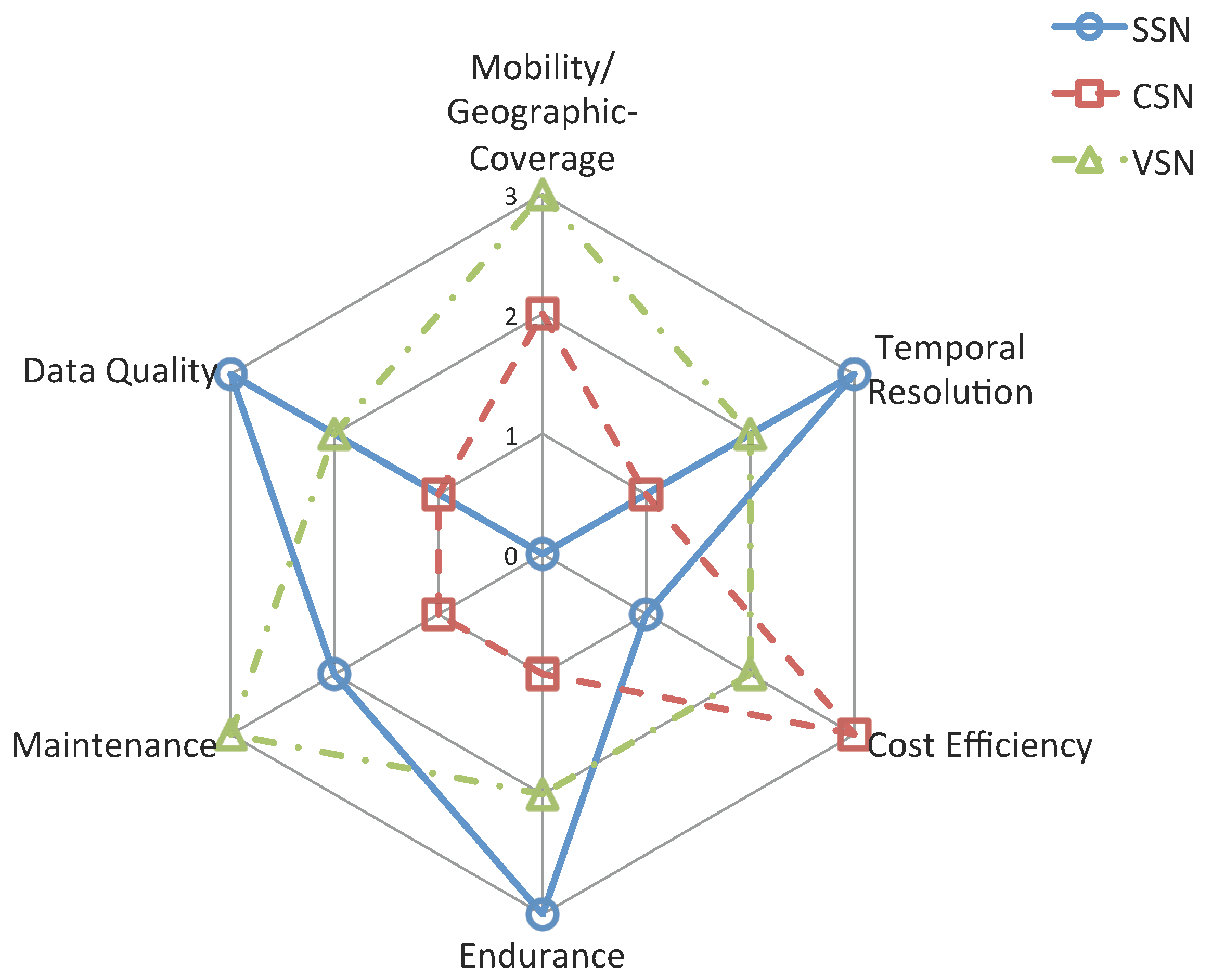
5. Comparison of The Three Types of Sensor Networks
5.1. Mobility/Geographic-Coverage
5.2. Temporal Resolution
5.3. Cost Efficiency
5.4. Endurance
5.5. Maintenance
5.6. Data Quality
6. Discussion and Conclusions
6.1. Issues and Challenges Need to Be Addressed
6.2. Abilities and Characteristics Need to Be Carried Forward
Conflicts of Interest
References
- World Health Organization. 7 Million Premature Deaths Annually Linked to Air Pollution. Available online: http://www.who.int/mediacentre/news/releases/2014/air-pollution/en/ (accessed on 20 August 2015).
- European Commission. Air quality: Commission Sends Final Warning to UK Over Levels of Fine Particle Pollution. Available online: http://europa.eu/rapid/press-release_IP-10-687_en.htm?locale=en (accessed on 20 August 2015).
- World Health Organization. Monitoring Ambient Air Quality for Health Impact Assessment. 1999. Available online: http://www.euro.who.int/__data/assets/pdf_file/0010/119674/E67902.pdf (accessed on 20 August 2015).
- World Health Organization. Ambient (Outdoor) Air Quality and Health. Available online: http://www.who.int/mediacentre/factsheets/fs313/en/ (accessed on 20 August 2015).
- Amorim, L.C.A.; Carneiro, J.P.; Cardeal, Z.L. An optimized method for determination of benzene in exhaled air by gas chromatography-mass spectrometry using solid phase microextraction as a sampling technique. J. Chromatogr. B 2008, 865, 141–146. [Google Scholar] [CrossRef] [PubMed]
- Environmental Protection Department of Hong Kong. Air Quality Health Index. Available online: http://www.aqhi.gov.hk/en.html (accessed on 22 August 2015).
- Beijing Municipal Environmental Protection Bureau. Beijing Environmental Statement 2013. Available online: http://www.bjepb.gov.cn/bjepb/resource/cms/2014/06/2014061911140819230.pdf (accessed on 22 August 2015).
- New York State Department of Environmental Conservation. New York State Air Quality Monitoring Center Home. Available online: http://www.dec.ny.gov/airmon/index.php (accessed on 22 August 2015).
- King’s College London. London Air Quality Network: Monitoring Sites. Available online: http://www.londonair.org.uk/london/asp/PublicEpisodes.asp (accessed on 22 August 2015).
- Hasenfratz, D.; Saukh, O.; Sturzenegger, S.; Thiele, L. Participatory Air Pollution Monitoring Using Smartphones. In Mobile Sensing: From Smartphones and Wearables to Big Data; ACM: Beijing, China, 2012. [Google Scholar]
- Völgyesi, P.; Nádas, A.; Koutsoukos, X.; Lédeczi, A. Air Quality Monitoring with SensorMap. In Proceedings of the 7th International Conference on Information Processing in Sensor Networks (IPSN ’08), St. Louis, MO, USA, 22–24 April 2008; pp. 529–530.
- Richards, M.; Ghanem, M.; Osmond, M.; Guo, Y.; Hassard, J. Grid-based analysis of air pollution data. Ecol. Model. 2006, 194, 274–286. [Google Scholar] [CrossRef]
- Dobre, A.; Arnold, S.J.; Smalley, R.J.; Boddy, J.W.D.; Barlow, J.F.; Tomlin, A.S.; Belcher, S.E. Flow field measurements in the proximity of an urban intersection in London, UK. Atmos. Environ. 2005, 39, 4647–4657. [Google Scholar] [CrossRef]
- Air Quality Expert Group. Nitrogen Dioxide in the United Kingdom; Technical Report; Department for the Environment, Food and Rural Affairs: London, UK, 2004. [Google Scholar]
- Yu, O.; Sheppard, L.; Lumley, T.; Koenig, J.Q.; Shapiro, G.G. Effects of Ambient Air Pollution on Symptoms of Asthma in Seattle-Area Children Enrolled in the CAMP Study. Environ. Health Perspect. 2000, 108, 1209–1214. [Google Scholar] [CrossRef] [PubMed]
- PopeIII, C.A.; Verrier, R.L.; Lovett, E.G.; Larson, A.C.; Raizenne, M.E.; Kanner, R.E.; Schwartz, J.; Villegas, G.; Gold, D.R.; Dockery, D.W. Heart rate variability associated with particulate air pollution. Am. Heart J. 1999, 138, 890–899. [Google Scholar] [CrossRef]
- Peters, A.; Dockery, D.W.; Muller, J.E.; Mittleman, M.A. Increased Particulate Air Pollution and the Triggering of Myocardial Infarction. Circulation 2001, 103, 2810–2815. [Google Scholar] [CrossRef] [PubMed]
- United States Environmental Protection Agency. Next Generation Air Measuring Research. Available online: http://www2.epa.gov/air-research/next-generation-air-measuring-researchr/ (accessed on 12 July 2015).
- Ma, Y.; Richards, M.; Ghanem, M.; Guo, Y.; Hassard, J. Air Pollution Monitoring and Mining Based on Sensor Grid in London. Sensors 2008, 8, 3601–3623. [Google Scholar] [CrossRef]
- Bravo, M.A.; Fuentes, M.; Zhang, Y.; Burr, M.J.; Bell, M.L. Comparison of exposure estimation methods for air pollutants: Ambient monitoring data and regional air quality simulation. Environ. Res. 2012, 116, 1–10. [Google Scholar] [CrossRef] [PubMed]
- Budde, M.; El Masri, R.; Riedel, T.; Beigl, M. Enabling Low-cost Particulate Matter Measurement for Participatory Sensing Scenarios. In Proceedings of the 12th International Conference on Mobile and Ubiquitous Multimedia (MUM ’13), Luleå, Sweden, 2–5 December 2013; ACM: New York, NY, USA, 2013; pp. 19:1–19:10. [Google Scholar]
- International Sensor Technology. Hazardous Gas Data. 1997. Available online: http://www.intlsensor.com/pdf/hazgasdata.pdf (accessed on 25 August 2015).
- United States Environmental Protection Agency. What are the Six Common Air Pollutants? Available online: http://www.epa.gov/airquality/urbanair/ (accessed on 25 August 2015).
- United States Environmental Protection Agency. Carbon Monoxide Home. Available online: http://www.epa.gov/airquality/carbonmonoxide/ (accessed on 27 August 2015).
- United States Environmental Protection Agency. Nitrogen Dioxide Home. Available online: http://www.epa.gov/airquality/nitrogenoxides/ (accessed on 27 August 2015).
- United States Environmental Protection Agency. Ground Level Ozone. Available online: http://www.epa.gov/airquality/ozonepollution/ (accessed on 27 August 2015).
- United States Environmental Protection Agency. Sulfur Dioxide Home. Available online: http://www.epa.gov/airquality/sulfurdioxide/ (accessed on 27 August 2015).
- United States Environmental Protection Agency. Particulate Matter Home. Available online: http://www.epa.gov/airquality/particlepollution/ (accessed on 27 August 2015).
- United States Environmental Protection Agency. Lead Home. Available online: http://www.epa.gov/airquality/lead/ (accessed on 27 August 2015).
- Johnson, D.L.; Ambrose, S.H.; Bassett, T.J.; Bowen, M.L.; Crummey, D.E.; Isaacson, J.S.; Johnson, D.N.; Lamb, P.; Saul, M.; Winter-Nelson, A.E. Meanings of Environmental Terms. J. Environ. Qual. 1997, 26, 581–589. [Google Scholar] [CrossRef]
- United States Environmental Protection Agency. Air Quality Index (AQI)—A Guide to Air Quality and Your Health. Available online: http://www.airnow.gov/index.cfm?action=aqibasics.aqi (accessed on 1 September 2015).
- European Commission. Indices Definition. Available online: http://www.airqualitynow.eu/about_home.php (accessed on 1 September 2015).
- Ministry of Environmental Protection of the People’s Republic of China. PRC National Environmental Protection Standard: Technical Regulation on Ambient Air Quality Index. 2012. Available online: http://kjs.mep.gov.cn/hjbhbz/bzwb/dqhjbh/jcgfffbz/201203/W020120410332725219541.pdf (accessed on 1 September 2014). [Google Scholar]
- Environmental Protection Department of Hong Kong. About AQHI. Available online: http://www.aqhi.gov.hk/en/what-is-aqhi/about-aqhi.html (accessed on 1 September 2015).
- Wong, T.W.; Tam, W.W.S.; Yu, I.T.S.; Wong, A.H.S.; Lau, A.K.H.; Ng, S.K.W.; Yeung, D.; Wong, C.M. A Study of the Air Pollution Index Reporting System; Technical Report; Environmental Protection Department of Hong Kong: Hong Kong, China, 2012.
- Environmental Protection Department of Hong Kong. Health Advice. Available online: http://www.aqhi.gov.hk/en/health-advice/sub-health-advice.html (accessed on 1 September 2015).
- United States Environmental Protection Agency. National Ambient Air Quality Standards. Available online: http://www.epa.gov/air/criteria.html (accessed on 27 August 2015).
- World Health Organization. Air Quality Guidelines. 2005. Available online: http://www.who.int/phe/health_topics/outdoorair/outdoorair_aqg/en/ (accessed on 27 August 2015).
- World Health Organization. Indoor Air Quality Guidelines. 2005. Available online: http://www.euro.who.int/__data/assets/pdf_file/0009/128169/e94535.pdf (accessed on 27 August 2015).
- World Health Organization. Exposure to Lead: A Major Public Health Concern. 2010. Available online: http://www.who.int/ipcs/assessment/public_health/lead/en/ (accessed on 27 August 2014).
- European Commission. Air Quality Standards. Available online: http://ec.europa.eu/environment/air/quality/standards.htm (accessed on 27 August 2015).
- Ministry of Environmental Protection of the People’s Republic of China. Ambient Air Quality Standards. 2012. Available online: http://kjs.mep.gov.cn/hjbhbz/bzwb/dqhjbh/dqhjzlbz/201203/t20120302_224165.htm (accessed on 27 August 2015). [Google Scholar]
- Environmental Protection Department of Hong Kong. Hong Kong’s Air Quality Objectives. Available online: http://www.epd.gov.hk/epd/english/environmentinhk/air/air_quality_objectives/air_quality_objectives.html (accessed on 27 August 2015).
- United States Environmental Protection Agency. List of Designated Reference and Equivalent Methods. Available online: http://www.epa.gov/ttnamti1/files/ambient/criteria/reference-equivalent-methods-list.pdf (accessed on 8 September 2015).
- Environmental Protection Department of Hong Kong. Air Quality Monitoring Equipment. Available online: http://www.aqhi.gov.hk/en/monitoring-network/air-quality-monitoring-equipment.html (accessed on 8 September 2015).
- Aleixandre, M.; Gerboles, M. Review of Small Commercial Sensors for Indicative Monitoring of Ambient Gas. Chem. Eng. Trans. 2012, 30, 169–174. [Google Scholar]
- Bender, F.; Barié, N.; Romoudis, G.; Voigt, A.; Rapp, M. Development of a preconcentration unit for a SAW sensor micro array and its use for indoor air quality monitoring. Sens. Actuators B: Chem. 2003, 93, 135–141. [Google Scholar] [CrossRef]
- Lee, Y.J.; Kim, H.B.; Roh, Y.R.; Cho, H.M.; Baik, S. Development of a SAW gas sensor for monitoring SO2 gas. Sens. Actuators A: Phys. 1998, 64, 173–178. [Google Scholar] [CrossRef]
- Fanget, S.; Hentz, S.; Puget, P.; Arcamone, J.; Matheron, M.; Colinet, E.; Andreucci, P.; Duraffourg, L.; Myers, E.; Roukes, M.L. Gas sensors based on gravimetric detection-A review. Sens. Actuators B Chem. 2011, 160, 804–821. [Google Scholar] [CrossRef]
- Boussaad, S.; Tao, N.J. Polymer Wire Chemical Sensor Using a Microfabricated Tuning Fork. Nano Lett. 2003, 3, 1173–1176. [Google Scholar] [CrossRef]
- Ren, M.; Forzani, E.S.; Tao, N. Chemical Sensor Based on Microfabricated Wristwatch Tuning Forks. Anal. Chem. 2005, 77, 2700–2707. [Google Scholar] [CrossRef] [PubMed]
- Shiina, T. LED mini-lidar as minimum setup. In Proceedings of the SPIE 9246, Amsterdam, Netherlands, 22 September 2014; Lidar Technologies, Techniques, and Measurements for Atmospheric Remote Sensing X, 92460F, Edinburgh, UK. 2014; pp. 92460F-1–92460F-6. [Google Scholar]
- Chiang, C.W.; Das, S.K.; Chiang, H.W.; Nee, J.B.; Sun, S.H.; Chen, S.W.; Lin, P.H.; Chu, J.C.; Su, C.S.; Su, L.S. A new mobile and portable scanning lidar for profiling the lower troposphere. Geosci. Instrum. Methods Data Syst. 2015, 4, 35–44. [Google Scholar] [CrossRef]
- Rionda, A.; Marin, I.; Martinez, D.; Aparicio, F.; Alija, A.; Garcia Allende, A.; Minambres, M.; Paneda, X.G. UrVAMM-A full service for environmental-urban and driving monitoring of professional fleets. In Proeedings of the 2013 International Conference on New Concepts in Smart Cities: Fostering Public and Private Alliances (SmartMILE), Gijon, Spain, 11–13 December 2013; pp. 1–6.
- Ltd., D.T. DUVAS Series. Available online: http://www.duvastechnologies.com/ (accessed on 18 June 2015).
- Data Sheet of BAM-1020 Beta Attenuation Monitor. 2013. Available online: http://www.metone.com/documents/BAM-1020_Datasheet.pdf (accessed on 10 September 2014).
- AEROCET 831 Aerosol Mass Monitor. 2014. Available online: http://www.metone.com/docs/831_datasheet.pdf (accessed on 10 September 2015).
- OPC-N2 Particle Monitor. 2015. Available online: http://www.alphasense.com/WEB1213/wp-content/uploads/2015/05/OPC-N2.pdf (accessed on 9 August 2015).
- Sharp DN7C3CA006 PM2.5 Sensor Module. 2014. Available online: http://media.digikey.com/pdf/Data%20Sheets/Sharp%20PDFs/DN7C3CA006_Spec.pdf (accessed on 9 August 2015).
- Data Sheet of Model 602 BetaPLUS Particle Measurement System. 2012. Available online: http://www.teledyne-api.com/pdfs/602_Literature_RevB.pdf (accessed on 10 September 2015).
- Sharp GP2Y1010AU Compact Dust Sensor for Air Conditioners. Available online: http://media.digikey.com/pdf/Data%20Sheets/Sharp%20PDFs/GP2Y1010AU.pdf (accessed on 9 August 2015).
- Data Sheet of ModelT300U Ultra-Sensitive Carbon Monoxide Analyzer. 2011. Available online: http://www.teledyne-ml.com/pdfs/T300U.pdf (accessed on 10 September 2015).
- Aeroqual Carbon Monoxide Sensor Head 0–25 ppm. 2014. Available online: http://www.aeroqual.com/product/carbon-monoxide-sensor-0-25ppm (accessed on 9 August 2015).
- CO-B4 Carbon Monoxide Sensor 4-Electrode. 2015. Available online: http://www.alphasense.com/WEB1213/wp-content/uploads/2015/04/COB41.pdf (accessed on 9 August 2015).
- MQ-7 Gas Sensor. Available online: http://www.ventor.co.in/Datasheet/MQ-7.pdf (accessed on 9 August 2015).
- Data Sheet of Model T500U CAPS Nitrogen Dioxide Analyzer. 2014. Available online: http://www.teledyne-api.com/pdfs/T500U_Literature.pdf (accessed on 10 September 2015).
- Aeroqual Nitrogen Dioxide Sensor Head 0-1 ppm. 2014. Available online: http://www.aeroqual.com/product/nitrogen-dioxide-sensor-0-1ppm (accessed on 9 August 2015).
- NO2-B42F Nitrogen Dioxide Sensor 4-Electrode. 2015. Available online: http://www.alphasense.com/WEB1213/wp-content/uploads/2015/03/NO2B42F.pdf (accessed on 9 August 2015).
- The MiCS-2714 is a compact MOS sensor. 2014. Available online: http://www.sgxsensortech.com/content/uploads/2014/08/1107_Datasheet-MiCS-2714.pdf (accessed on 9 August 2015).
- Data Sheet of Model 265E Chemiluminescence Ozone Analyzer. Available online: http://www.teledyne-api.com/pdfs/265E_Literature_RevC.pdf (accessed on 10 September 2014).
- Aeroqual Ozone Sensor Head 0-0.15 ppm. 2014. Available online: http://www.aeroqual.com/product/ozone-sensor-ozu (accessed on 9 August 2015).
- OX-B421 Oxidising Gas Sensor Ozone + Nitrogen Dioxide 4-Electrode. 2015. Available online: http://www.alphasense.com/WEB1213/wp-content/uploads/2015/04/OX-B421.pdf (accessed on 9 August 2015).
- MQ-131 Semiconductor Sensor for Ozone. Available online: http://www.datasheet-pdf.com/PDF/MQ131-Datasheet-HenanHanwei-770516 (accessed on 9 August 2015).
- Data Sheet of Model 6400T/6400E Sulfur Dioxide Analyzer. Available online: http://www.teledyne-ai.com/pdf/6400t_Rev-B.pdf (accessed on 10 September 2015).
- Aeroqual Sulfur Dioxide Sensor Head 0-10 ppm. 2014. Available online: http://www.aeroqual.com/product/sulfur-dioxide-sensor-0-10ppm (accessed on 9 August 2015).
- SO2-B4 Sulfur Dioxide Sensor 4-Electrode. 2014. Available online: http://www.alphasense.com/WEB1213/wp-content/uploads/2014/08/SO2B4.pdf (accessed on 9 August 2015).
- MQ-136 Semiconductor Sensor for Sulfur Dioxide. Available online: http://www.china-total.com/Product/meter/gas-sensor/MQ136.pdf (accessed on 9 August 2015).
- Chou, J. Electrochemical Sensors. In Hazardous Gas Monitors—A Practical Guide to Selection, Operation and Applications; McGraw-Hill and SciTech Publishing: New York, NY, USA, 1999; pp. 27–35. [Google Scholar]
- Chou, J. Catalytic Combustible Gas Sensors. In Hazardous Gas Monitors—A Practical Guide to Selection, Operation and Applications; McGraw-Hill and SciTech Publishing: New York, NY, USA, 1999; pp. 37–45. [Google Scholar]
- Chou, J. Solid-State Gas Sensors. In Hazardous Gas Monitors—A Practical Guide to Selection, Operation and Applications; McGraw-Hill and SciTech Publishing: New York, NY, USA, 1999; pp. 47–53. [Google Scholar]
- Chou, J. Infrared Gas Sensors. In Hazardous Gas Monitors—A Practical Guide to Selection, Operation and Applications; McGraw-Hill and SciTech Publishing: New York, NY, USA, 1999; pp. 55–72. [Google Scholar]
- Chou, J. Photoionization Detectors. In Hazardous Gas Monitors—A Practical Guide to Selection, Operation and Applications; McGraw-Hill and SciTech Publishing: New York, NY, US, 1999; pp. 73–81. [Google Scholar]
- Williams, R.; Kilaru, V.; Snyder, E.; Kaufman, A.; Dye, T.; Rutter, A.; Russell, A.; Hafner, H. Air Sensor Guidebook; Technical report, United States Environmental Protection Agency; 2004. [Google Scholar]
- Chou, J. Sensor Selection Guide. In Hazardous Gas Monitors—A Practical Guide to Selection, Operation and Applications; McGraw-Hill and SciTech Publishing: New York, NY, USA, 1999; Chapter 8; pp. 103–109. [Google Scholar]
- Gerboles, M.; Buzica, D. Evaluation of Micro-Sensors to Monitor Ozone in Ambient Air; Technical report, Joint Research Center, Institute for Environment and Sustainability; 2009. [Google Scholar]
- Air Quality Expert Group. Methods for Monitoring Particulate Concentrations. In Particulate Matter in the United Kingdom; Department for the Environment, Food and Rural Affairs: London, UK, 2005; pp. 125–129. [Google Scholar]
- Grover, B.D.; Kleinman, M.; Eatough, N.L.; Eatough, D.J.; Hopke, P.K.; Long, R.W.; Wilson, W.E.; Meyer, M.B.; Ambs, J.L. Measurement of total PM2.5 mass (nonvolatile plus semivolatile) with the Filter Dynamic Measurement System tapered element oscillating microbalance monitor. J. Geophys. Res: Atmos. 2005, 110, 148–157. [Google Scholar]
- Air Quality Expert Group. Methods for Monitoring Particulate Concentrations. In Particulate Matter in the United Kingdom; Department for the Environment, Food and Rural Affairs: London, UK, 2005; pp. 129–131. [Google Scholar]
- Air Quality Expert Group. Methods for Monitoring Particulate Concentrations. In Particulate Matter in the United Kingdom; Department for the Environment, Food and Rural Affairs: London, UK, 2005; pp. 131–133. [Google Scholar]
- Air Quality Expert Group. Methods for Monitoring Particulate Concentrations. In Particulate Matter in the United Kingdom; Department for the Environment, Food and Rural Affairs: London, UK, 2005; pp. 134–143. [Google Scholar]
- Air Quality Expert Group. Methods for Monitoring Particulate Concentrations. In Particulate Matter in the United Kingdom; Department for the Environment, Food and Rural Affairs: London, UK, 2005; pp. 133–137. [Google Scholar]
- United States Environmental Protection Agency. Compact Nephelometer System for On-Line Monitoring of Particulate Matter Emissions. 2004. Available online: http://cfpub.epa.gov//ncer_abstracts/index.cfm/fuseaction/display.abstractdetail/abstract/6539 (accessed on 25 September 2015). [Google Scholar]
- Choi, S.; Kim, N.; Cha, H.; Ha, R. Micro Sensor Node for Air Pollutant Monitoring: Hardware and Software Issues. Sensors 2009, 9, 7970–7987. [Google Scholar] [CrossRef] [PubMed]
- Ikram, J.; Tahir, A.; Kazmi, H.; Khan, Z.; Javed, R.; Masood, U. View: Implementing low cost air quality monitoring solution for urban areas. Environ. Syst. Res. 2012, 1, 10–15. [Google Scholar] [CrossRef]
- Hasenfratz, D.; Saukh, O.; Walser, C.; Hueglin, C.; Fierz, M.; Thiele, L. Pushing the Spatio-Temporal Resolution Limit of Urban Air Pollution Maps. In Proceedings of the 12th International Conference on Pervasive Computing and Communications (PerCom 2014), Budapest, Hungary, 24–28 March 2014; pp. 69–77.
- Burke, J.A.; Estrin, D.; Hansen, M.; Parker, A.; Ramanathan, N.; Reddy, S.; Srivastava, M.B. Participatory sensing. In Proceedings of the 4th ACM Conference on Embedded Network Sensor Systems (SenSys ’6), Boulder, CO, USA, 1–3 November 2006; pp. 1124–1127.
- Mendez, D.; Perez, A.J.; Labrador, M.A.; Marron, J.J. P-Sense: A participatory sensing system for air pollution monitoring and control. In Procedings of the 2011 IEEE International Conference on Pervasive Computing and Communications Workshops (PERCOM Workshops), Seattle, WA, USA, 21–25 March 2011; pp. 344–347.
- Hu, S.C.; Wang, Y.C.; Huang, C.Y.; Tseng, Y.C. A vehicular wireless sensor network for CO2 monitoring. IEEE Sens. 2009, 2009, 1498–1501. [Google Scholar]
- Wong, K.J.; Chua, C.C.; Li, Q. Environmental Monitoring Using Wireless Vehicular Sensor Networks. In Proceedings of the 5th International Conference on Wireless Communications, Networking and Mobile Computing, 2009 (WiCom ’09), Beijing, China, 24–26 September 2009; pp. 1–4.
- Hasenfratz, D. Enabling Large-Scale Urban Air Quality Monitoring with Mobile Sensor Nodes. Ph.D. Thesis, ETH-Zűrich, ZÃrich, Switzerland, 2015. [Google Scholar]
- Murty, R.N.; Mainland, G.; Rose, I.; Chowdhury, A.R.; Gosain, A.; Bers, J.; Welsh, M. CitySense: An Urban-Scale Wireless Sensor Network and Testbed. In Proceedings of the 2008 IEEE Conference on Technologies for Homeland Security, Waltham, MA, USA, 12–13 May 2008; pp. 583–588.
- Liu, J.H.; Chen, Y.F.; Lin, T.S.; Lai, D.W.; Wen, T.H.; Sun, C.H.; Juang, J.Y.; Jiang, J.A. Developed urban air quality monitoring system based on wireless sensor networks. In Proceedings of the 2011 Fifth International Conference on Sensing Technology (ICST), Palmerston North, New Zealand, 28 November 2011–1 December 2011; pp. 549–554.
- Kadri, A.; Yaacoub, E.; Mushtaha, M.; Abu-Dayya, A. Wireless sensor network for real-time air pollution monitoring. In Proceedings of the 2013 1st International Conference on Communications, Signal Processing, and their Applications (ICCSPA), Sharjah, UAE, 12–14 February 2013; pp. 1–5.
- Khedo, K.K.; Perseedoss, R.; Mungur, A. A Wireless Sensor Network Air Pollution Monitoring System. IJWMN 2010, 2, 1–15. [Google Scholar] [CrossRef]
- Mansour, S.; Nasser, N.; Karim, L.; Ali, A. Wireless Sensor Network-based air quality monitoring system. In Proceedings of the 2014 International Conference on Computing, Networking and Communications (ICNC), Honolulu, HI, USA, 3–6 February 2014; pp. 545–550.
- Libelium. Libelium Waspmote. Available online: http://www.libelium.com/products/waspmote/ (accessed on 27 May 2015).
- Jelicic, V.; Magno, M.; Brunelli, D.; Paci, G.; Benini, L. Context-Adaptive Multimodal Wireless Sensor Network for Energy-Efficient Gas Monitoring. IEEE Sens. J. 2013, 13, 328–338. [Google Scholar] [CrossRef]
- Postolache, O.A.; Pereira, J.M.D.; Girao, P.M.B.S. Smart Sensors Network for Air Quality Monitoring Applications. IEEE Trans. Instrum. Meas. 2009, 58, 3253–3262. [Google Scholar] [CrossRef]
- Jiang, Y.; Li, K.; Tian, L.; Piedrahita, R.; Yun, X.; Mansata, O.; Lv, Q.; Dick, R.P.; Hannigan, M.; Shang, L. MAQS: A Personalized Mobile Sensing System for Indoor Air Quality Monitoring. In Proceedings of the 13th International Conference on Ubiquitous Computing (UbiComp ’11), Beijing, China, 17–21 September 2011; pp. 271–280.
- Aberer, K.; Sathe, S.; Chakraborty, D.; Martinoli, A.; Barrenetxea, G.; Faltings, B.; Thiele, L. OpenSense: Open Community Driven Sensing of Environment. In Proceedings of the ACM SIGSPATIAL International Workshop on GeoStreaming (GIS-IWGS), San Jose, CA, USA, 2 November 2010; pp. 39–42.
- Honicky, R.; Brewer, E.A.; Paulos, E.; White, R. N-smarts: Networked Suite of Mobile Atmospheric Real-time Sensors. In Proceedings of the Second ACM SIGCOMM Workshop on Networked Systems for Developing Regions (NSDR’08), Seattle, WA, USA, 18 August 2008; pp. 25–30.
- Maisonneuve, N.; Stevens, M.; Niessen, M.E.; Hanappe, P.; Steels, L. Citizen Noise Pollution Monitoring. In Proceedings of the 10th Annual International Conference on Digital Government Research: Social Networks: Making Connections Between Citizens, Data and Government (dg.o ’09), Puebla, Mexico, 17–21 May 2009; pp. 96–103.
- Tsow, F.; Forzani, E.; Rai, A.; Wang, R.; Tsui, R.; Mastroianni, S.; Knobbe, C.; Gandolfi, A.J.; Tao, N.J. A Wearable and Wireless Sensor System for Real-Time Monitoring of Toxic Environmental Volatile Organic Compounds. IEEE Sens. J. 2009, 9, 1734–1740. [Google Scholar] [CrossRef]
- United States Environmental Protection Agency. Buildings and their Impact on the Environment: A Statistical Summary. 2009. Available online: http://www.epa.gov/greenbuilding/pubs/gbstats.pdf (accessed on 16 June 2015). [Google Scholar]
- Lo Re, G.; Peri, D.; Vassallo, S. Urban Air Quality Monitoring Using Vehicular Sensor Networks. In Advances onto the Internet of Things; Gaglio, S., Lo Re, G., Eds.; Springer International Publishing: Gewerbestrasse, Switzerland, 2014; pp. 311–323. [Google Scholar]
- Hu, S.C.; Wang, Y.C.; Huang, C.Y.; Tseng, Y.C. Measuring air quality in city areas by vehicular wireless sensor networks. Mobile Applications: Status and Trends. J. Syst. Softw. 2011, 84, 2005–2012. [Google Scholar] [CrossRef]
- Devarakonda, S.; Sevusu, P.; Liu, H.; Liu, R.; Iftode, L.; Nath, B. Real-time Air Quality Monitoring Through Mobile Sensing in Metropolitan Areas. In Proceedings of the 2nd ACM SIGKDD International Workshop on Urban Computing (UrbComp ’13), Chicago, IL, USA, 11 August 2013; pp. 15:1–15:8.
- Al-Ali, A.R.; Zualkernan, I.; Aloul, F. A Mobile GPRS-Sensors Array for Air Pollution Monitoring. IEEE Sens. J. 2010, 10, 1666–1671. [Google Scholar] [CrossRef]
- Liu, J.; Diamond, J. Revolutionizing China’s Environmental Protection. Science 2008, 319, 37–38. [Google Scholar] [CrossRef] [PubMed]
- Al-Saadi, J.; Szykman, J.; Pierce, R.B.; Kittaka, C.; Neil, D.; Chu, D.A.; Remer, L.; Gumley, L.; Prins, E.; Weinstock, L.; MacDonald, C.; Wayland, R.; Dimmick, F.; Fishman, J. Improving National Air Quality Forecasts with Satellite Aerosol Observations. Bull. Am. Meteorol. Soc. 2005, 86, 1249–1261. [Google Scholar] [CrossRef]
- Engel-Cox, J.; Hoff, R.; Weber, S.; Zhang, H.; Prados, A. Three Dimensional Air Quality System (3D-AQS). 2007. Available online: http://alg.umbc.edu/3d-aqs/doc/3daqs_agu_winter2007.pdf (accessed on 17 July 2015).
- Calpini, B.; Simeonov, V.; Jeanneret, F.; Kuebler, J.; Sathya, V.; van den Bergh, H. Ozone LIDAR as an Analytical Tool in Effective Air Pollution Management: The Geneva 96 Campaign. CHIMIA Int. J. Chem. 1997, 51, 700–704. [Google Scholar]
© 2015 by the authors; licensee MDPI, Basel, Switzerland. This article is an open access article distributed under the terms and conditions of the Creative Commons by Attribution (CC-BY) license (http://creativecommons.org/licenses/by/4.0/).
Share and Cite
Yi, W.Y.; Lo, K.M.; Mak, T.; Leung, K.S.; Leung, Y.; Meng, M.L. A Survey of Wireless Sensor Network Based Air Pollution Monitoring Systems. Sensors 2015, 15, 31392-31427. https://doi.org/10.3390/s151229859
Yi WY, Lo KM, Mak T, Leung KS, Leung Y, Meng ML. A Survey of Wireless Sensor Network Based Air Pollution Monitoring Systems. Sensors. 2015; 15(12):31392-31427. https://doi.org/10.3390/s151229859
Chicago/Turabian StyleYi, Wei Ying, Kin Ming Lo, Terrence Mak, Kwong Sak Leung, Yee Leung, and Mei Ling Meng. 2015. "A Survey of Wireless Sensor Network Based Air Pollution Monitoring Systems" Sensors 15, no. 12: 31392-31427. https://doi.org/10.3390/s151229859