
Feasibility Study of EO SARs as Opportunity Illuminators in Passive Radars: PAZ-Based Case Study

Abstract
:1. Introduction
- Low development, implementation and maintenance costs.
- Easy deployment without any particular power requirement, using solar panels and batteries, and without complex civil engineering.
- Small size and low weight.
- Low probability of intercept (LPI).
- Invulnerability against the progressive erosion of communication systems, which are demanding the use of traditional radar frequencies.
- Avoidance of electromagnetic compatibility or environment impact problems.
- Alternative geometries.
- Different scattering mechanisms.
- Ground resolution comparable to that of a monostatic system in fixed-receiver bistatic systems [16].
- Advantageous sensitivity requirements due to the shorter distance from target to receiver.
- Low cost experimentation of single and multichannel techniques (only a passive antenna with multiple sub-apertures with no space qualification).
- No data-link/data storage limitations.
- Data immediately available at the ground receiver.
2. Passive Radar Performance Principle

- is the number of samples.
- m represents the time bin associated with a delay .
- p is the Doppler bin corresponding to Doppler shift .
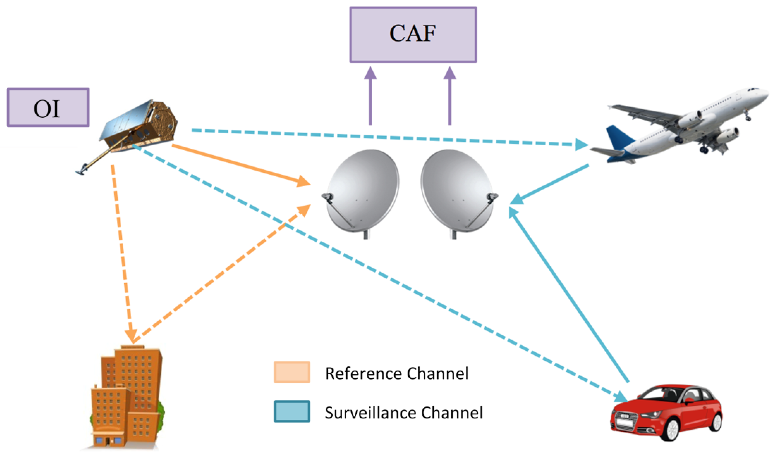
- and are the reference and surveillance signals, respectively.
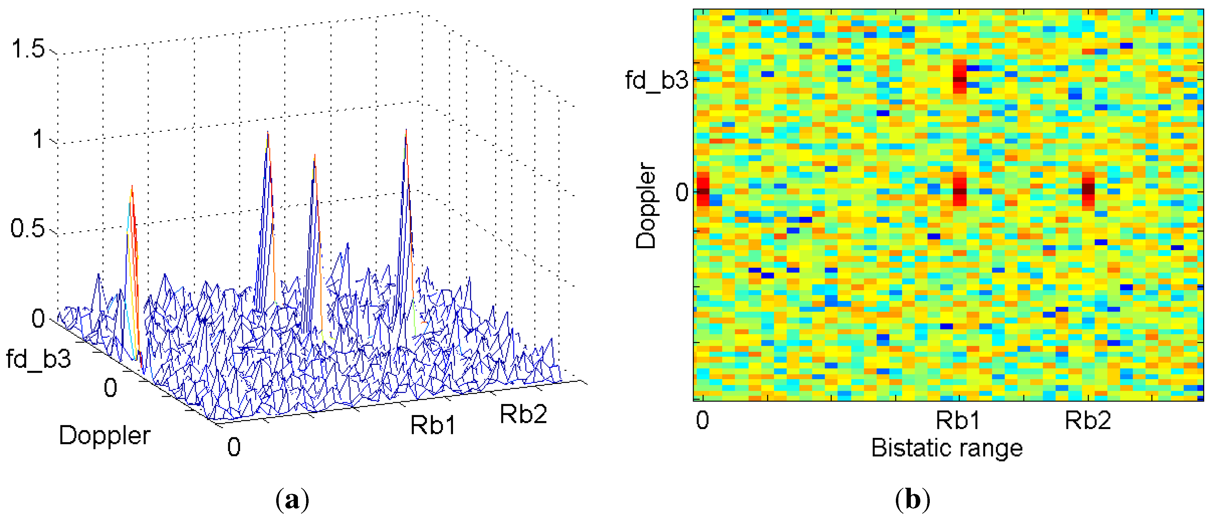
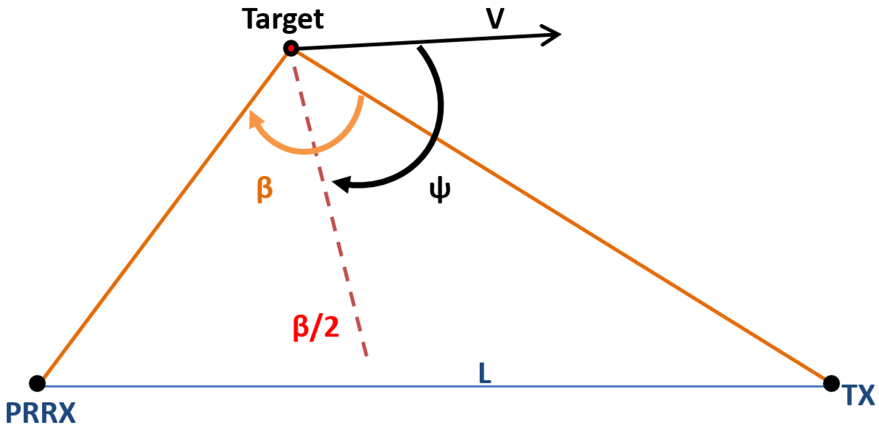
- Two stationary targets are at bistatic ranges and . These bistatic ranges are calculated as , where is the bistatic delay calculated in Equation (2) as a function of the target-OI, the target-PR and the OI-PR or baseline distances, denoted as and L, respectively. c is the velocity of light. Stationary targets appear in the zero Doppler line of the range-Doppler map.
- One moving target is detected at a bistatic range . Its echo appears in the range-Doppler map at , where is the bistatic Doppler generated by target movement relative to the OI and the PR.
- The direct signal transmitted by the OI is captured by the reference and surveillance channels. The surveillance antenna is designed for rejecting this direct signal, but as it can be 100–80 dB higher than the target radar echoes, the level captured by the surveillance antenna can be significant compared to the target echo ones. This signal, known as the direct path interference (DPI) signal, correlates perfectly with the reference antenna signal, and as a result, a peak appears in the range-Doppler map of the CAF, located at zero bistatic range and zero Doppler.
2.1. Bistatic Range Resolution

2.2. Bistatic Doppler Resolution

2.3. Bistatic Radar Equation
2.4. System Coverage Limited by Sensitivity

2.5. Bistatic Radar Cross-Section
- Some target aspect angles that generate a low monostatic RCS and a high bistatic specular RCS at specific bistatic angles.
- Targets that are designed for low monostatic RCS over a range of aspect angles.
- Shadowing that sometimes occurs in a monostatic geometry and not in a bistatic one.


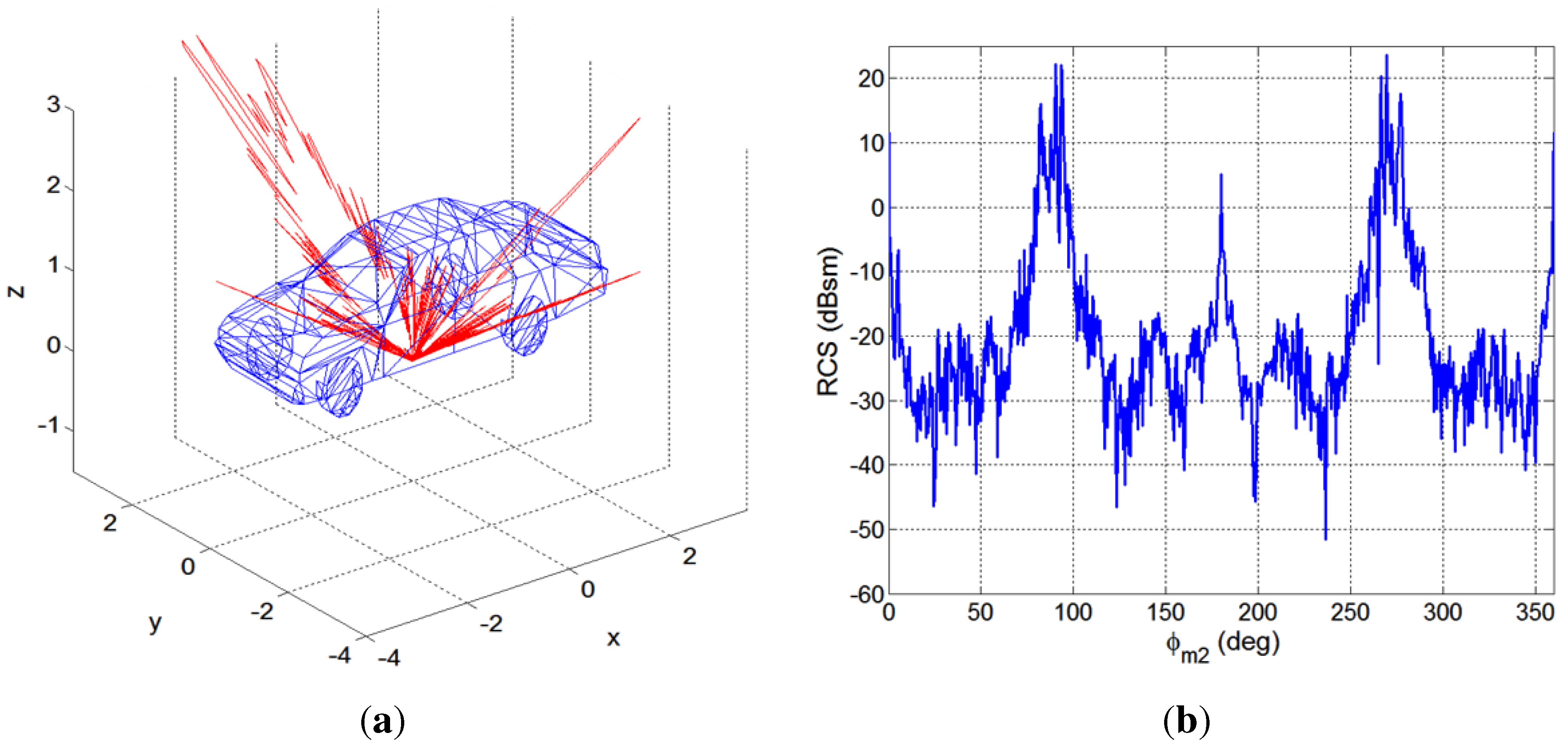
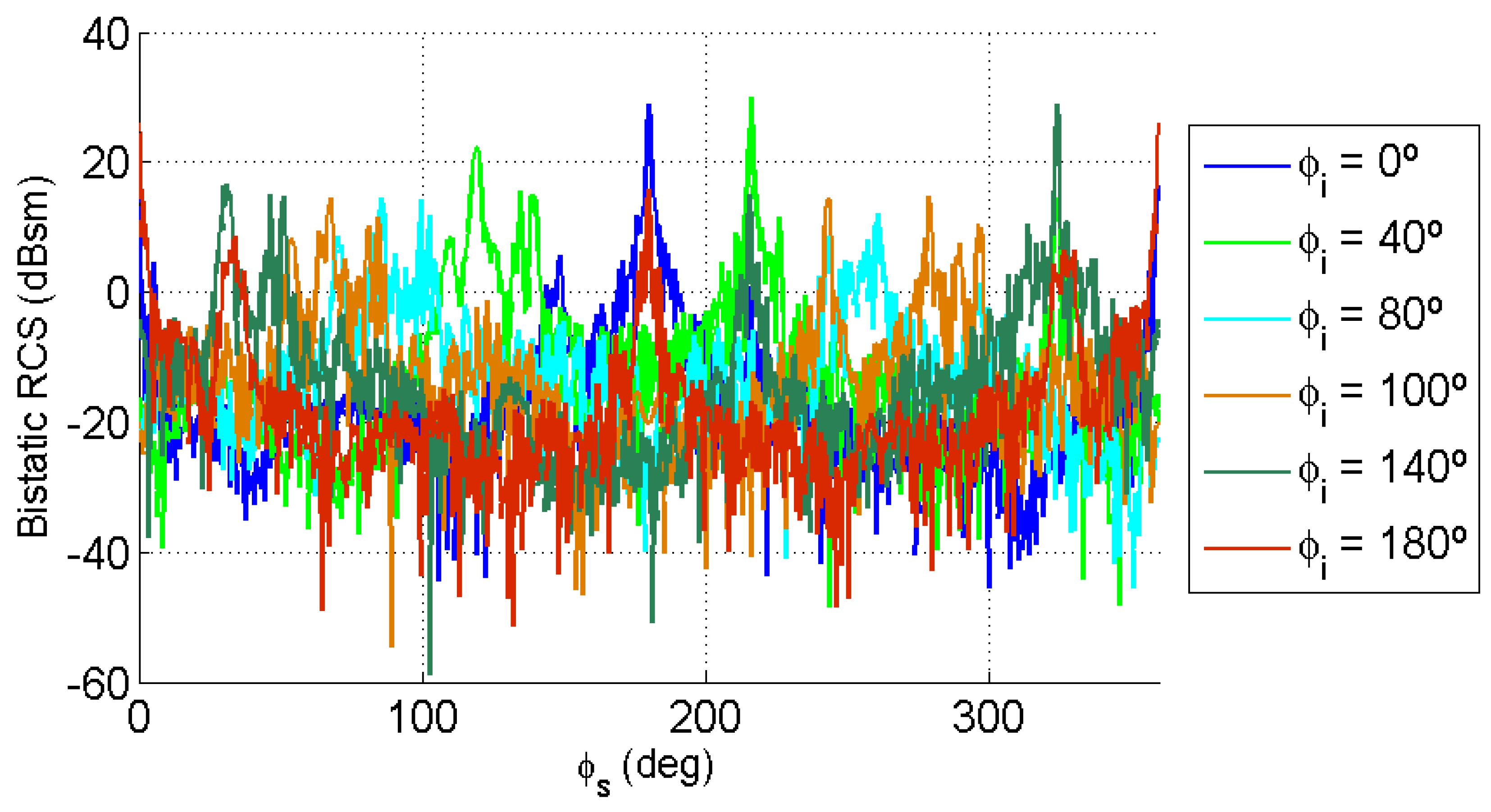
- For each value of incidence elevation angle, and , the incidence azimuth angle, , was varied from to , taking into consideration the symmetry of the car in the XY plane.
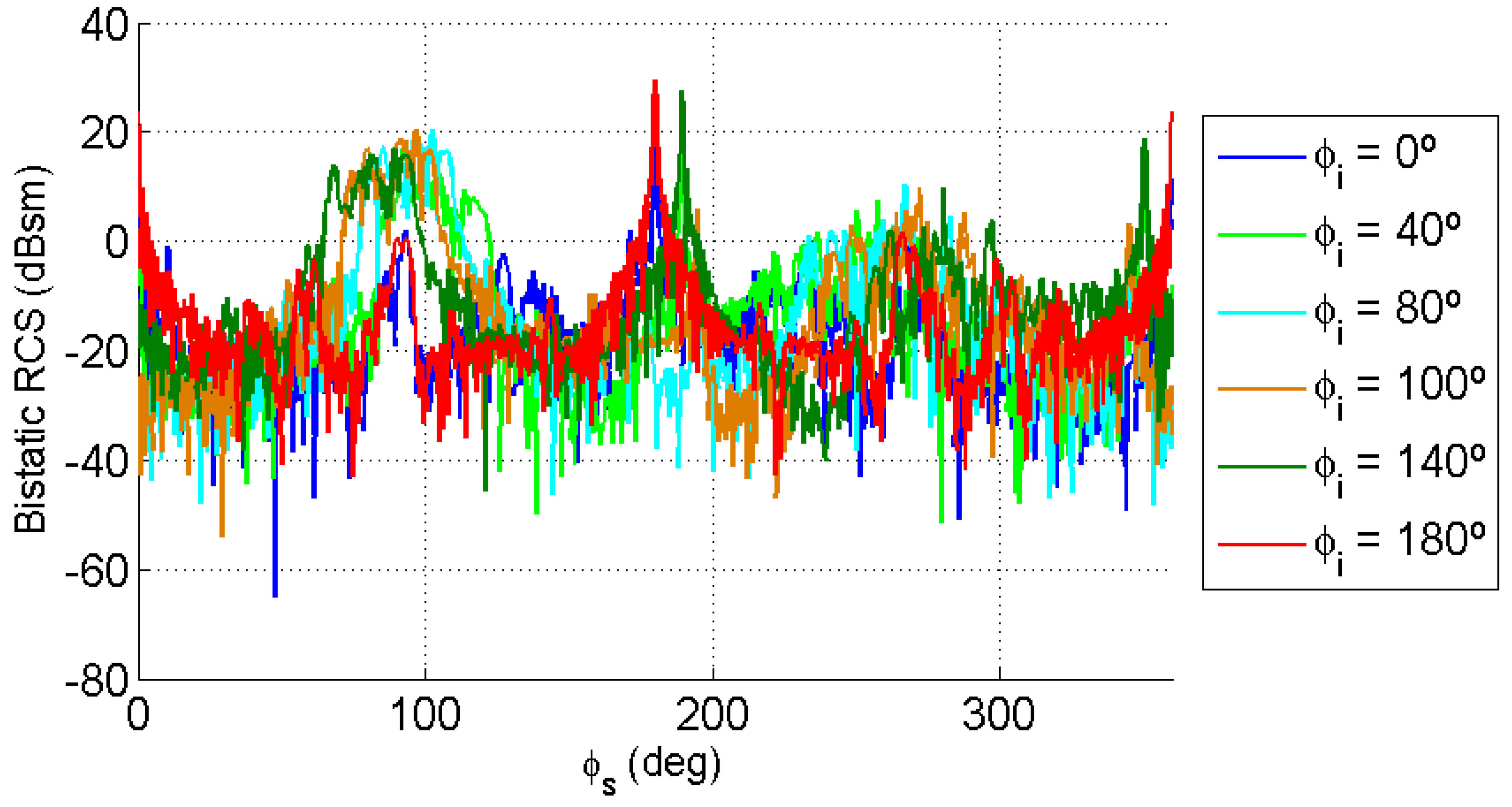

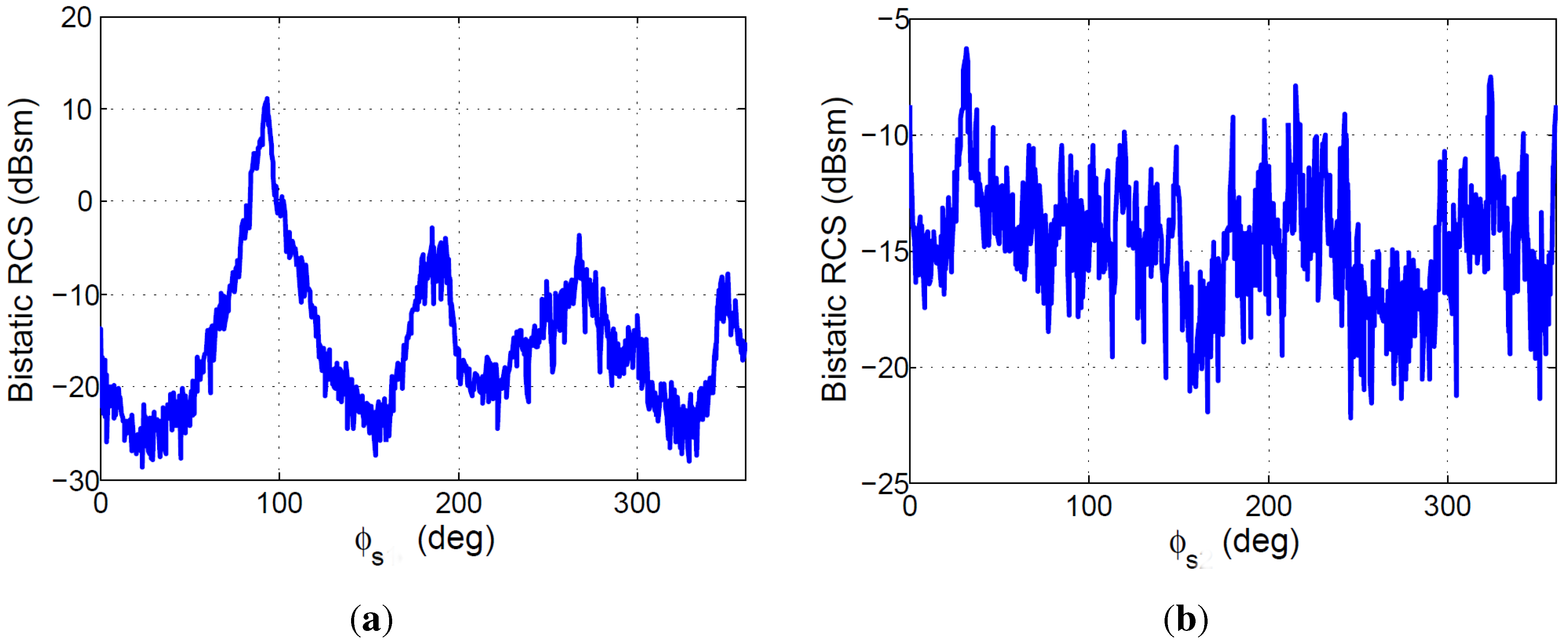
- For each scattering direction, , and incidence elevation angle , an average bistatic RCS was calculated as the mean value of the bistatic RCSs estimated for the set of values ranging from to . The study carried out for was denoted as Bistatic-1 and the study for was denoted as Bistatic-2. Results are presented in Figure 12.


| RCS | Monostatic 1 | Bistatic 1 | Monostatic 2 | Bistatic 2 |
|---|---|---|---|---|
| Maximum | 37.385 dBsm | 11.074 dBsm | 23.611 dBsm | −6.293 dBsm |
| Minimum | −50.229 dBsm | −28.678 dBsm | −51.619 dBsm | −22.193 dBsm |
| Average | −3.331 dBsm | −15.522 dBsm | −20.532 dBsm | −14.658 dBsm |
3. PAZ Description
- To identify areas of interest considering the Spanish environment and compromises.
- To provide data to the scientific community for educational, scientific and technological purposes.
- To research SAR systems’ characterization and calibration, operating modes’ definition, multi-static configurations and multi-sensor developments.
- To collaborate with high level SAR institutions.
- To develop a set of research-based demonstrators to prove SAR technology capabilities in different applications.
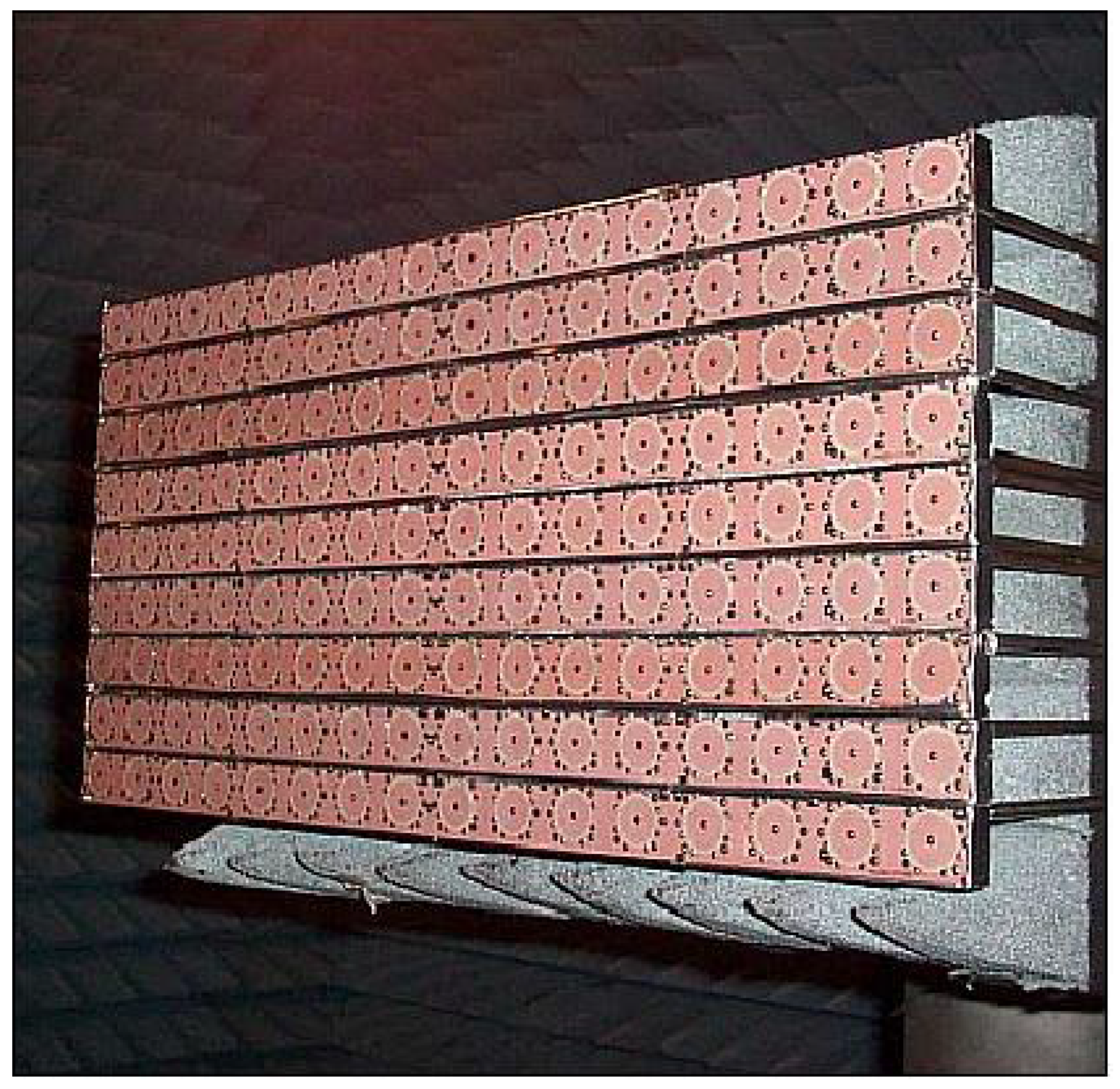
3.1. PAZ Antenna

- Subarray directivity higher than 20.1 dB for vertical and horizontal polarizations.
- Losses lower than 1 dB.
- Peak power equal to 2.26 kW.
- is the element efficiency term due to possible mismatching effects.
- represents the scan loss effect, which is typically modeled as a function of , being the main beam pointing direction with respect to the array broadside direction.
- represents the directivity of each single radiating element.
- N is the number of single radiating elements in the array.
3.2. Transmitted Signal
| Central frequency | 9.65 GHz |
| Maximum bandwidth | 300 MHz |
| Peak power | 1.9 kW |
| Pulse length | 15 µs–67 µs |
| Service factor | – |
| Pulse repetition frequency | 2 kH– kH |
3.3. Orbit Parameters
| Nominal height | 514 km |
| Orbits per day | 15 + 2/11 |
| Incidence angle | 20–45 (full perf.) 15–60 (accessible) |
3.4. PAZ Imaging Modes
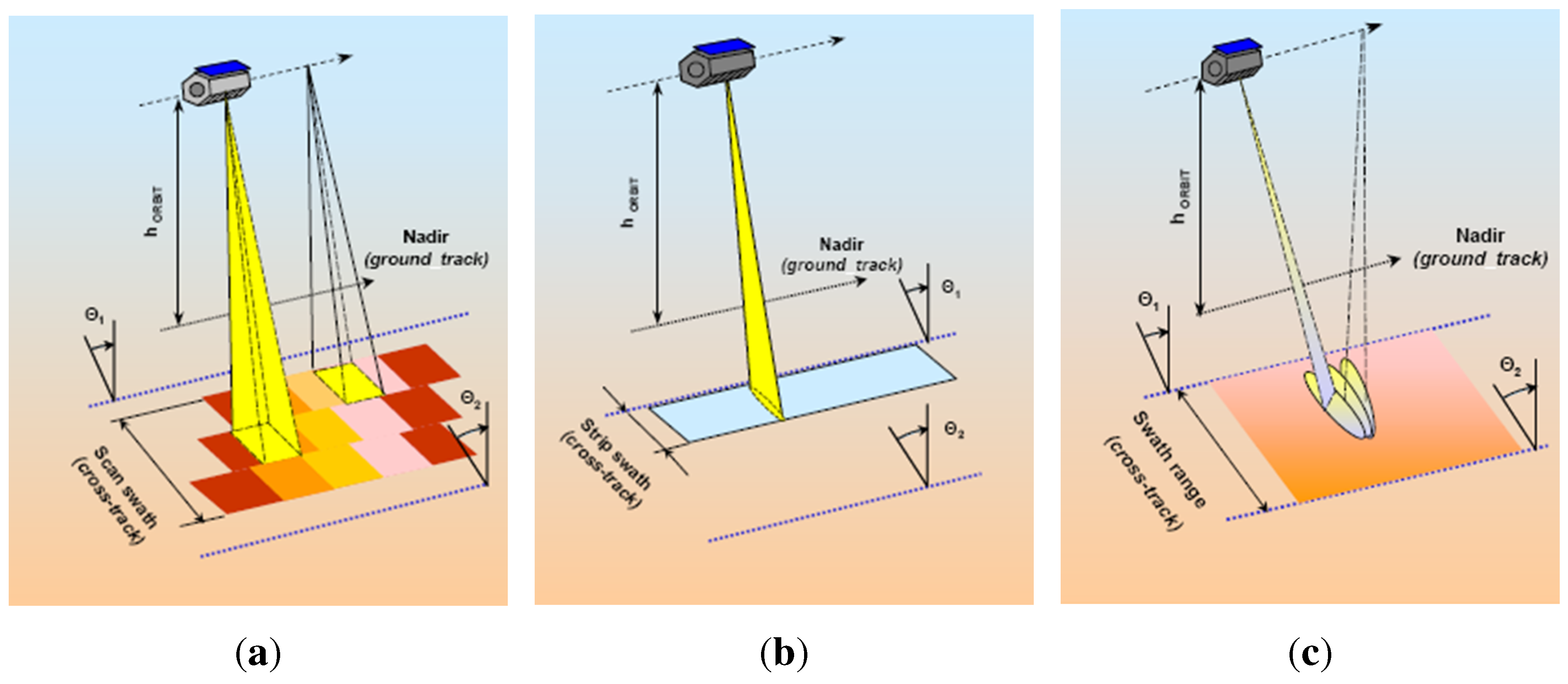
- Stripmap: The antenna beam is pointed to a fixed angle in elevation and azimuth, resulting in a strip with constant quality in azimuth (azimuth resolution up to 3 m, scene size up to 30 km × 50 km). Single (HH, VV) and dual (HH/VV, HH/HV, VV/VH) polarization modes are possible.
- ScanSAR: The electronic antenna elevation steering is used to switch after bursts of pulses between swathes with different incidence angles. This mode has an azimuth resolution up to 18 m, with a scene size of 100 km × 150 km. It can only acquire images with single polarization (HH, VV).
- Spotlight: Azimuth phased array beam steering is used to increase the illumination time and the azimuth resolution, at the cost of azimuth scene size (azimuth resolution up to 2 m, scene size of 10 km × 10 km). Single (HH, VV) and dual polarization (HH/VV) operating modes are possible.
- High resolution spotlight: this mode has an azimuth resolution up to 1 m, with a scene size of 10 km × 5 km and is able to operate with single (HH, VV) and dual polarization (HH/VV).
4. Feasibility of PAZ as an Opportunity Illuminator in a Passive Bistatic Radar System
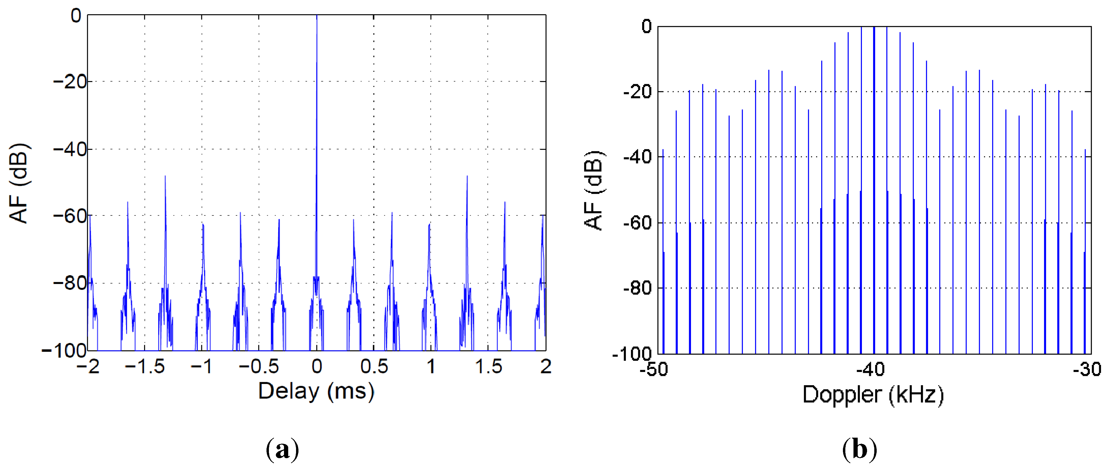
4.1. OI Signal Waveform
- Pulse repetition frequency, PRF = 3.03886 kHz
- Duty cycle, .
- Pulse duration, T = 62.523 µs.
- Modulation factor, Hz/s
- Bandwidth, MHz
- Number of Linear Frequency Modulation (LFM) pulses, 50.
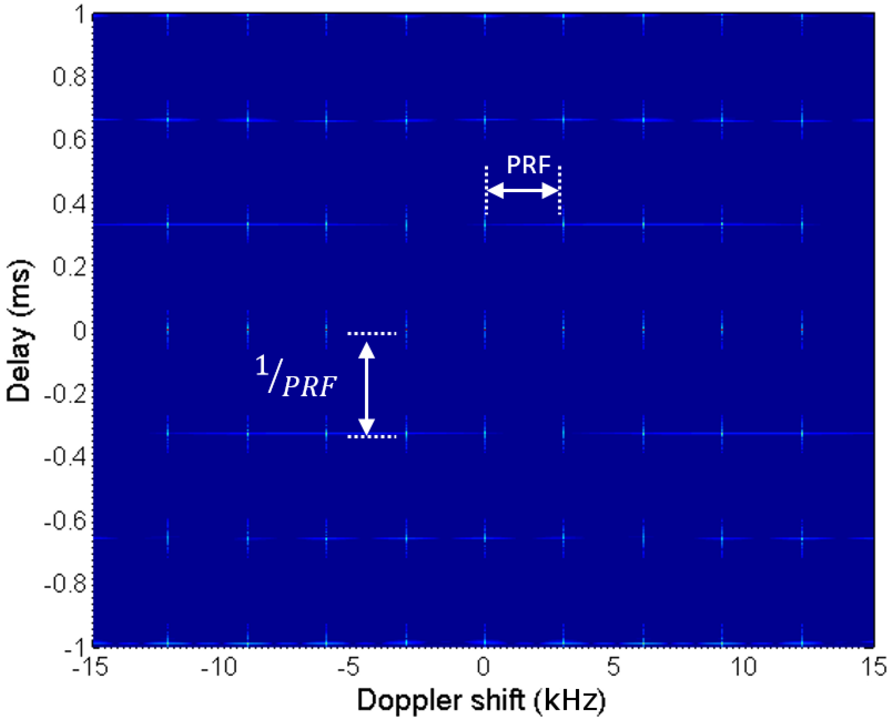
- Periodic ambiguity peaks appear along the time delay dimension, with a period equal to .
- Periodic ambiguity peaks appear along the Doppler shift dimension, with a period equal to .


4.2. OI Availability
- The time availability: determined by the sensor orbit parameters and the scheduled data acquisition processes. This study is directly related to the knowledge of the OI position that is studied in Section 4.3.
- The instrumented spatial coverage: determined by the EO satellite footprint, which depends on the sensor movement and acquisition mode. It is studied in Section 4.4.
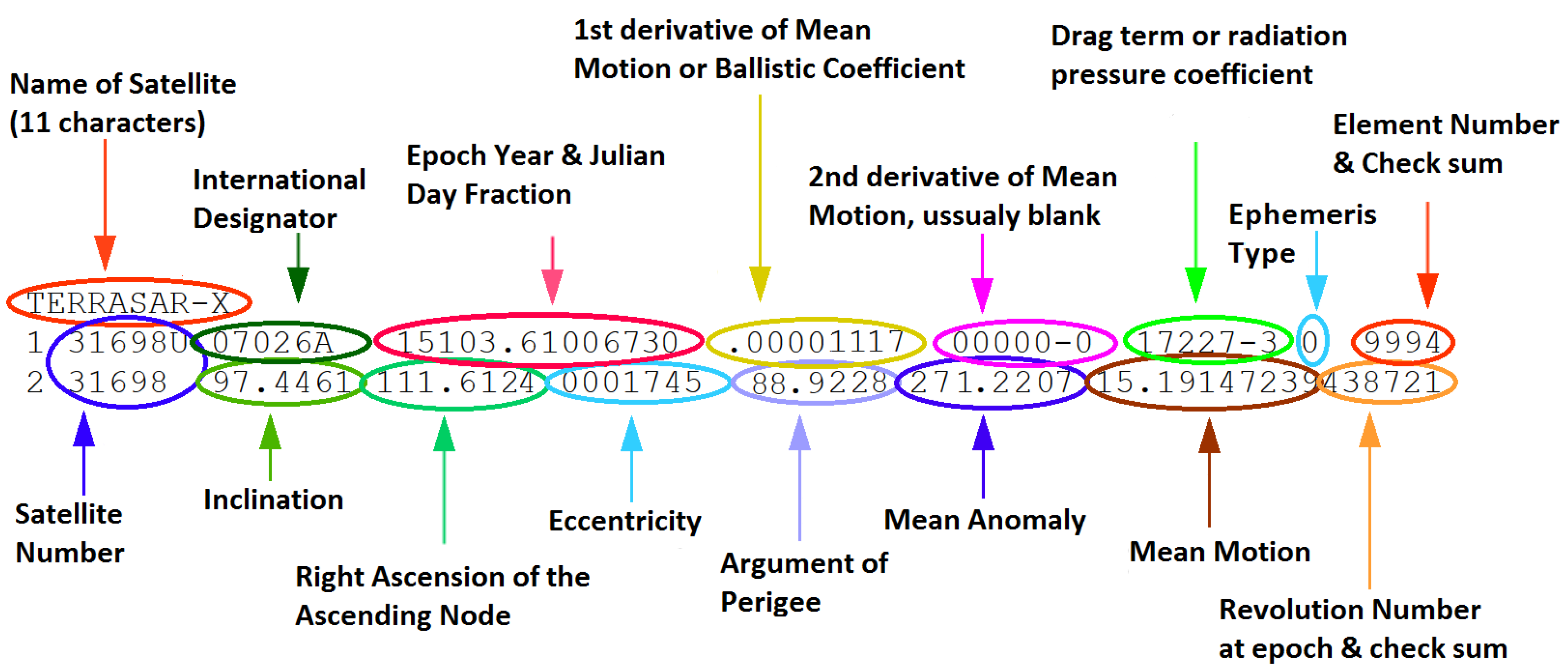
4.3. Knowledge of the OI Position

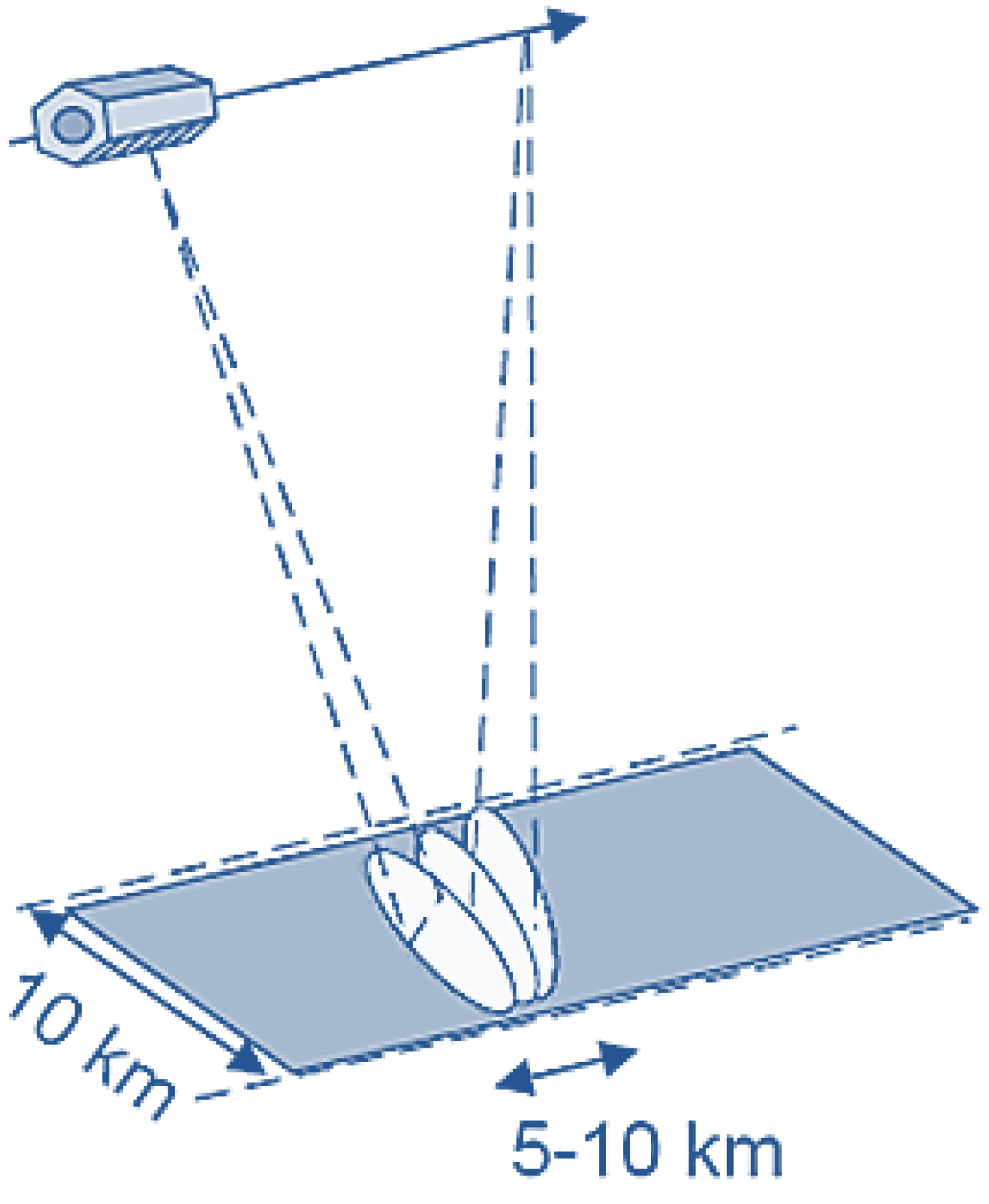
4.4. Instrumented Coverage Area
- The reference channel must include tracking techniques to guarantee the reference signal reception.
- The surveillance channel must reject the OI direct signal (direct path interference (DPI)) as the OI beam moves. The PR receiver and the area of interest are in the same coverage oval, so both are illuminated by the OI. Targets to be sought are on the surface or at low altitudes compared to the OI position, making the rejection of the direct OI signal feasible (incidence angles in ). The DPI rejection requires a surveillance antenna system capable of generating notches toward the satellite elevation and a receiver with properly-designed filtering techniques.
- If the OI antenna beam cannot be considered stationary or quasi-stationary during the acquisition time (stripmap or ScanSAR imaging modes), the coverage area will vary with the footprint movement.

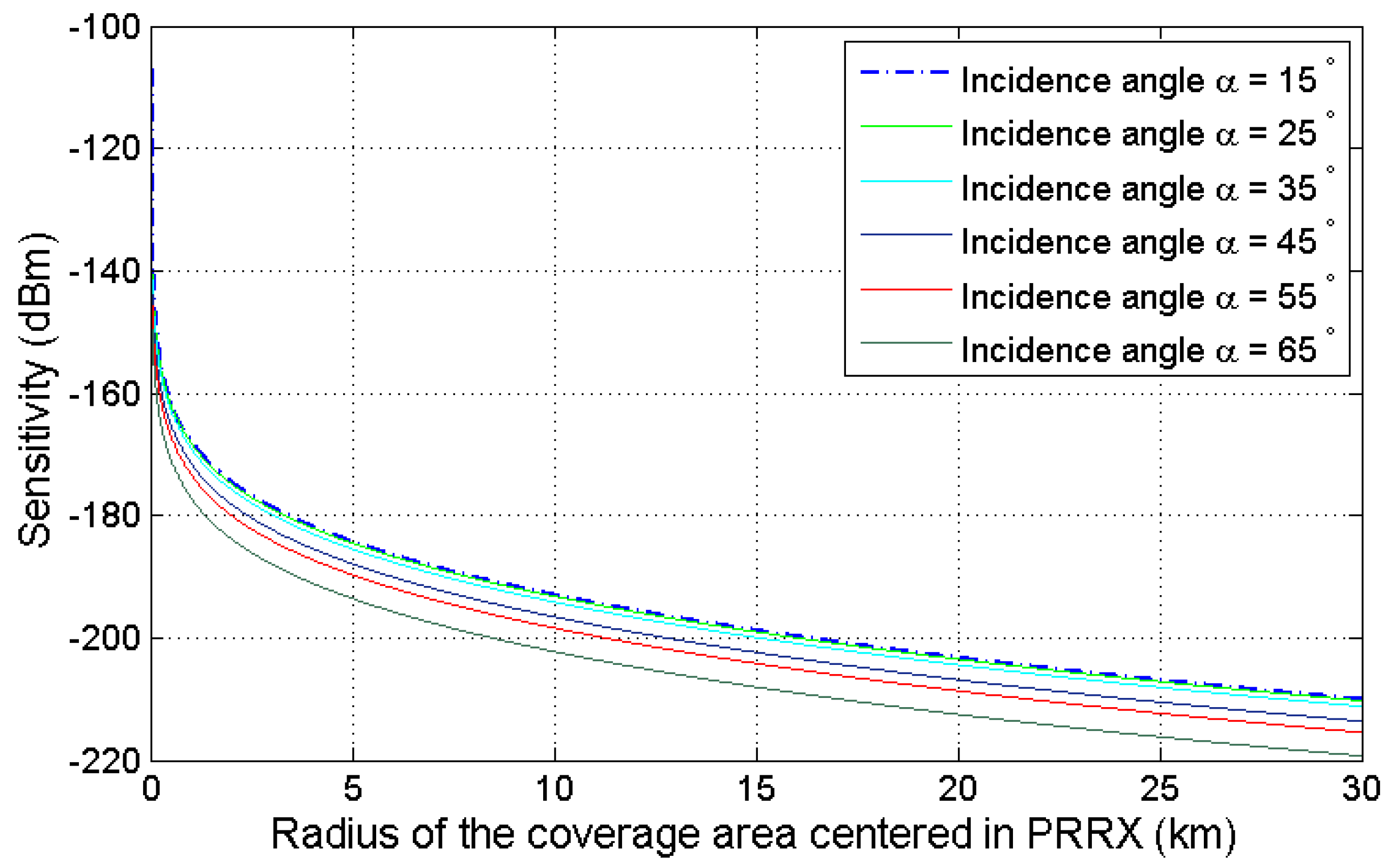
4.5. Incident Power Density and Required Sensitivity
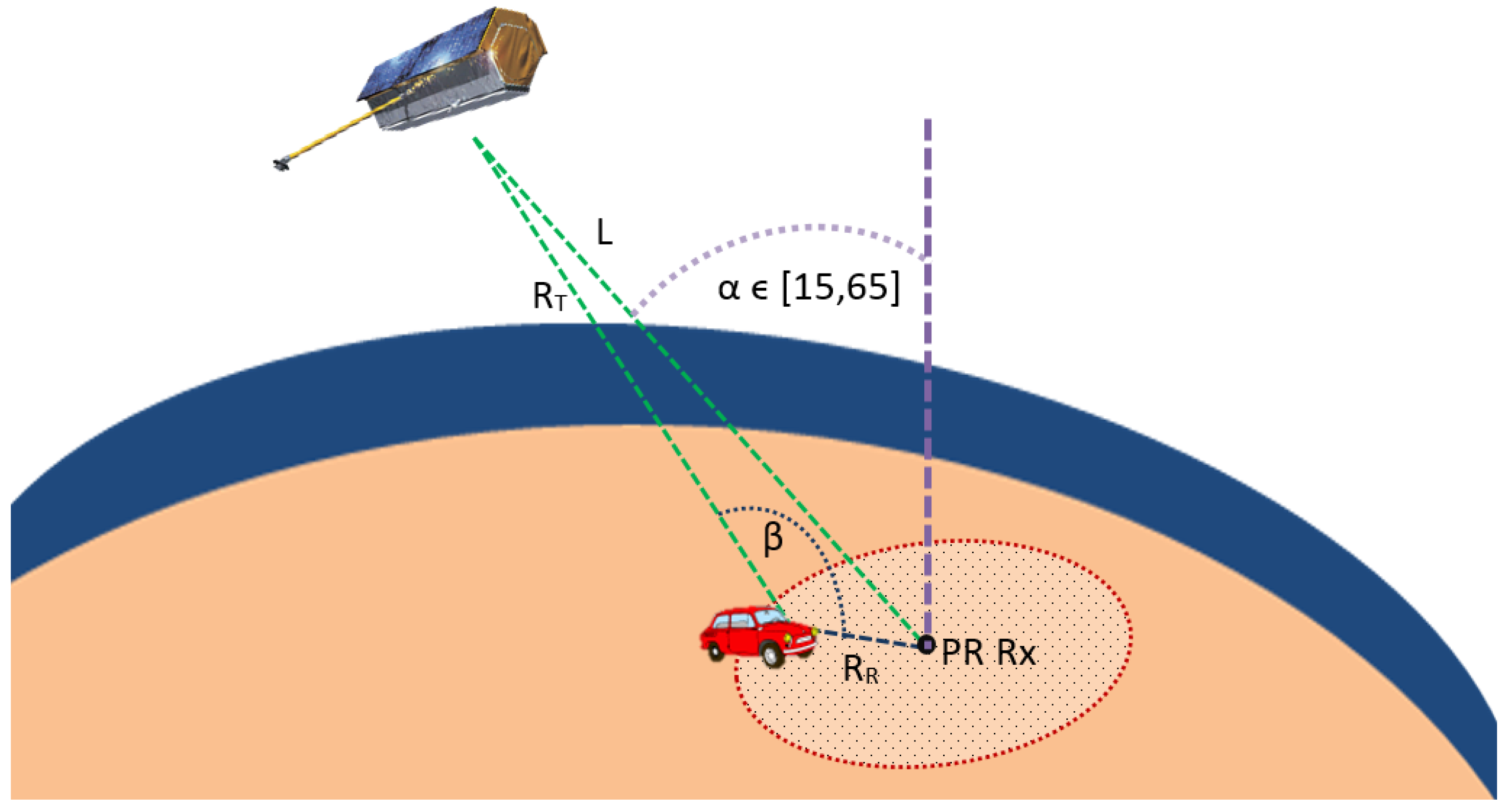
- The incidence angle of the PAZ antenna beam, α, can vary in (Figure 6). This parameter determines the baseline, the OI-target distances and the associated propagation losses.
- The estimated values of Equivalent Isotropic Radiated Power (EIRP) calculated in Section 3.1 range from dBm for , to dBm for .
- A receiver gain () of 23 dB was considered. Average bistatic RCS values were calculated for each incidence angle following the methodology explained in Section 2.5. Estimated values for the car model used in Section 2.5 are presented in Table 4.
- The PR receiver was located at N and W.
| RCS | ||||||
|---|---|---|---|---|---|---|
| Maximum | 11.074 dBsm | −0.046 dBsm | −5.539 dBsm | −7.631 dBsm | −8.385 dBsm | −6.293 dBsm |
| Minimum | −28.678 dBsm | −29.317 dBsm | −28.164 dBsm | −26.995 dBsm | −26.685 dBsm | −22.193 dBsm |
| Average | −15.522 dBsm | −15.912 dBsm | −15.897 dBsm | −16.729 dBsm | −16.132 dBsm | −14.658 dBsm |
5. Case Study Example
- The satellite moved from N, W to N, W.
- Satellite altitude remained approximately constant and equal to 513.4 km.
- The acquisition started at the time when the elevation angle of the satellite with respect to the PR receiver location was maximum. The elevation variations were of some hundredths of degree around .
- The azimuth of the satellite with respect to the North varied , from to . This variation was higher due to the polar orbit of the sensor.
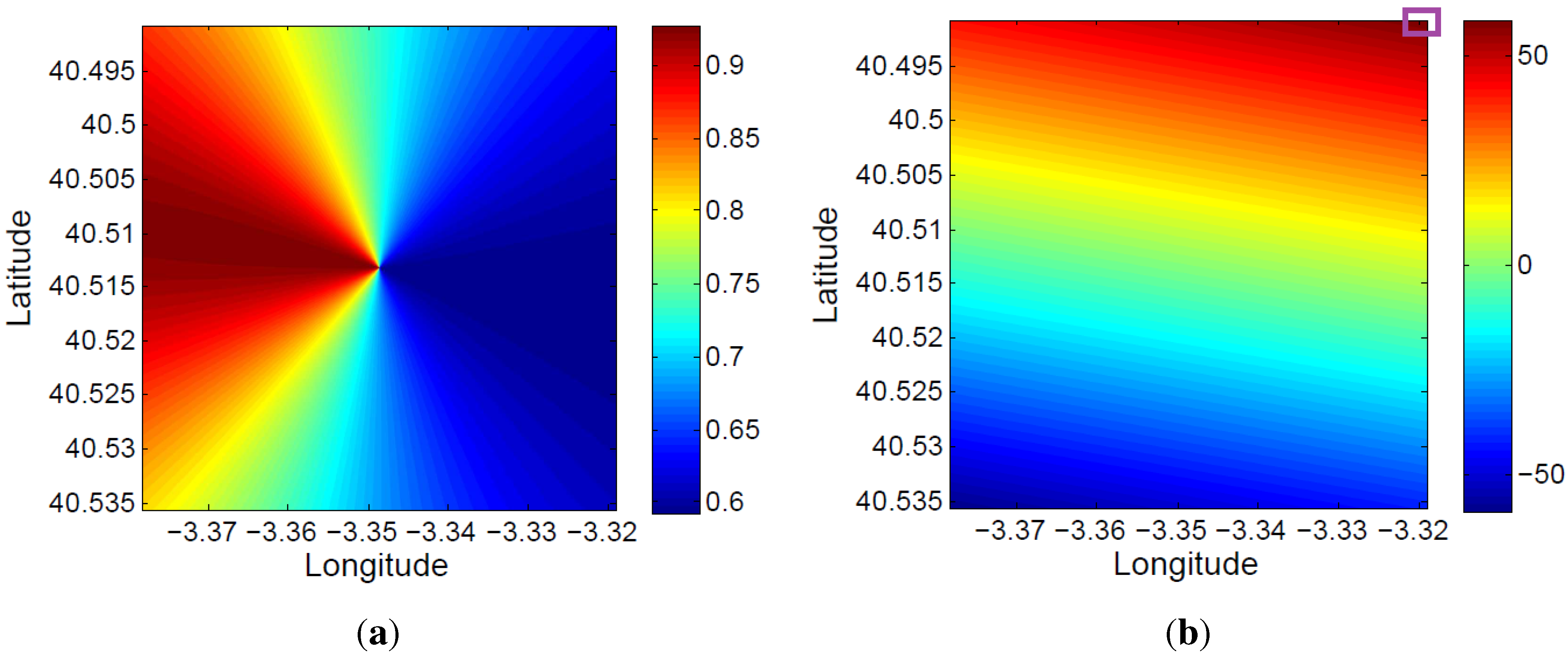
- The area of interest was divided into m cells.
- The system geometry was calculated assuming that a non-moving ground target was located at the center of each cell.
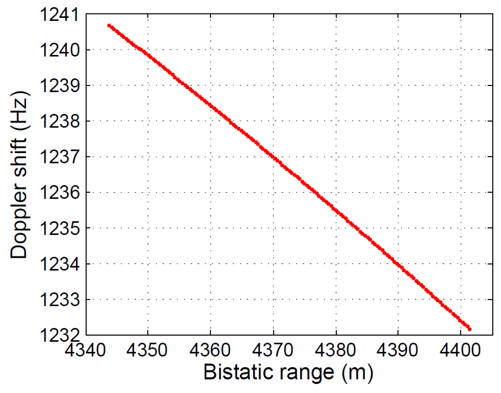
- The system geometry was recalculated each 0.01 s (150 time slots were analyzed) in order to take into account the satellite dynamics.


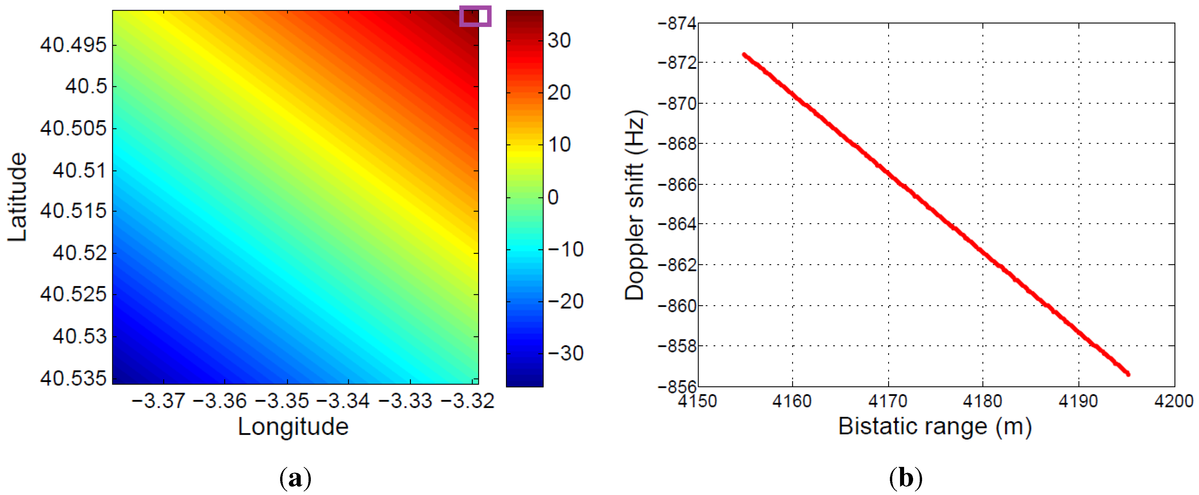
- Virtual movement analysis for a bistatic radar scenario using the same satellite, but assuming a different acquisition date: The new date and time parameters are: 3 June 2015, 17:34:15. Figure 24 shows the total variation of the bistatic range and the virtual movement of the same stationary target as in the previous study, during the same acquisition time. In this case, the maximum magnitude of the bistatic range variation is approximately 35 m, lower than the approximated 55 m obtained in the previous study.

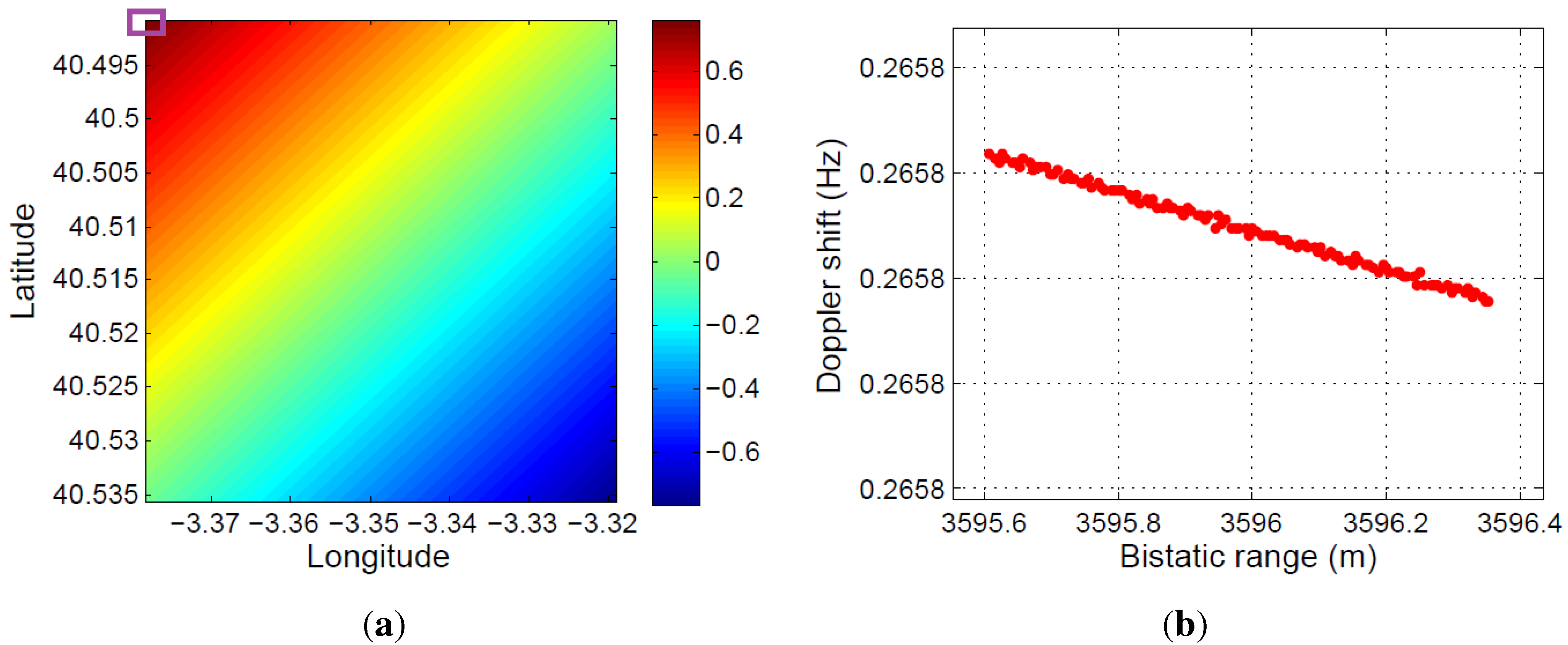
- Virtual movement analysis for a bistatic radar scenario using a GPS satellite: A new study case is considered exploiting the signal transmitted by Navstart 59 (USA 192). This is a medium-orbit satellite. The date and time parameters are: 25 May 2015, 12:20:00. The characteristics of the orbit and the transmitted signal parameters used in the study are summarized in Table 5 and Table 6, respectively. Results are presented in Figure 25. In this case, the stationary target is assumed to be located on the upper left corner of Figure 25a, in order to perform the analysis for a case characterized by a big variation of the considered parameters. For the same acquisition time used in previous examples, the obtained virtual displacement is significantly lower, less than 1 m.
| Central frequency | 1557 MHz |
| Bandwidth | 2 MHz |
| Power | 27 W |
| Modulation | Spread spectrum |
| Transmission rate | 50 bps |
| Nominal height | 20,200 km |
| Orbits per day | 2 |

6. Conclusions
- The transmitted signal is characterized by periodic ambiguity peaks that limit the coverage area and the target dynamics. After a study of instrumented coverage and system sensitivity, the limits imposed by the signal AF are beyond the limits imposed by these other factors, so the ambiguity peaks have no practical effect on system performance.
- OI availability: A study of potential bistatic geometries was carried out in order to determine the time availability and the instrumented spatial coverage. The orbital parameters, the acquisition modes and the operation schedule impose critical limitations on the OI availability. Taking into consideration these limitations, the following potential applications are proposed:
- −
- A PR system exploiting the signal emitted by PAZ can be used as a low-cost, easily deployable and configurable calibration tool in the commissioning phase of the SAR sensor or in posterior maintenance processes. The cost associated with the PR receiver is expected to be reduced due to the availability of commercial systems for direct receiving of sensor X-band data.
- −
- PR based on PAZ can also provide additional information, especially that related to the speed and trajectory of moving targets, to improve the information extraction from the acquired SAR images in the operational phase. This application can be really important in areas of special interest for monitoring specific phenomena.
- −
- As a PR can exploit the signal transmitted by other SAR sensors, GNSS and communication satellites, BSAR images can be generated to fill time gaps during which PAZ is not available.
- Instrumented coverage area: This is determined by the OI antenna footprint. The spotlight acquisition mode simplifies the geometry of the system, because it allows the definition of a constant coverage area during SAR sensor operation. For stripmap or ScanSAR operation, the knowledge of the sensor position makes it possible to study the movement of the coverage area, providing an increase of the achievable coverage.Different study cases were defined to analyze the impact of OI orbit: two study cases based on TerraSAR-X with different orbit parameters and a study case based on a GPS satellite.
- Incident power density and required sensitivity: The available power at the PR antenna was estimated as a function of the target-to-PR distance, proving the feasibility of PAZ as an IO from this point of view, allowing coverages of 15 km with affordable system sensitivities.
Acknowledgments
Author Contributions
Conflicts of Interest
References
- Willis, N.J. Bistatic Radar; Scitech Publishing Inc.: Raleigh, NC, USA, 2005. [Google Scholar]
- Cristallini, D.; Caruso, M.; Falcone, P.; Langellotti, D.; Bongioanni, C.; Colone, F.; Scafe, S.; Lombardo, P. Space-Based Passive Radar Enabled by the New Generation of Geostationary Broadcast Satellites. In Proceedings of the IEEE Aerospace Conference, Big Sky, MT, USA, 6–13 March 2010; Volume 1, pp. 1–11.
- Glennon, E.; Dempster, A.; Rizo, C. Feasibility of Air Target Detection Using GPS as a Bistatic Radar. J. Glob. Position. Syst. 2006, 1–2, 119–126. [Google Scholar] [CrossRef]
- Barcena-Humanes, J.L.; del Rey-Maestre, N.; Jarabo-Amores, M.; Mata-Moya, D.; Gomez-del Hoyo, P. Passive radar imaging capabilities using space-borne commercial illuminators in surveillance applications. In Proceedings of the Signal Processing Symposium (SPSympo), Debe, Poland, 10–12 June 2015; pp. 1–5.
- Pierdicca, N.; De-Titta, L.; Pulvirenti, L.; Della-Pietra, G. Bistatic Radar Configuration for Soil Moisture Retrieval: Analysis of the Spatial Coverage. Sensors 2009, 9, 7250–7265. [Google Scholar] [CrossRef] [PubMed]
- Copernicus. European Earth Observation Program. Available online: http://www.copernicus.eu/ (accessed on 27 October 2015).
- Maillard, P.; Alencar-Silva, T.; Clausi, D. An Evaluation of Radarsat-1 and ASTER Data for Mapping Veredas (Palm Swamps). Sensors 2008, 8, 6055–6076. [Google Scholar] [CrossRef]
- Earth-Observation-Portal. eo Sharing Earth Observation Resources. “PAZ SAR Satellite Mission of Spain”. Available online: https://directory.eoportal.org/web/eoportal/satellite-missions/p/paz (accessed on 4 September 2015).
- Breit, H.; Fritz, T.; Balss, U.; Lachaise, M.; Niedermeier, A.; Vonavka, M. TerraSAR-X SAR Processing and Products. IEEE Trans. Geosci. Remote Sens. 2010, 48, 727–740. [Google Scholar] [CrossRef]
- Rodriguez-Cassola, M.; Prats, P.; Schulze, D.; Tous-Ramon, N.; Steinbrecher, U.; Marotti, L.; Nannini, M.; Younis, M.; Lopez-Dekker, P.; Zink, M.; et al. First bistatic spaceborne SAR experiments with TanDEM-X. IEEE Geosci. Remote Sens. Lett. 2012, 9, 33–37. [Google Scholar] [CrossRef] [Green Version]
- Dubois-Fernandez, P.; Cantalloube, H.; Vaizan, B.; Krieger, G.; Horn, R.; Wendler, M.; Giroux, V. ONERA-DLR bistatic SAR campaign: Planning, data acquisition, and first analysis of bistatic scattering behavior of natural and urban targets. IEE Proc. Radar Sonar Navig. 2006, 153, 214–223. [Google Scholar] [CrossRef]
- Antoniou, M.; Cherniakov, M. GNSS-based bistatic SAR: A signal processing view. EURASIP J. Adv. Signal Process. 2013, 2013, 1–16. [Google Scholar] [CrossRef]
- Chai, S.; Chen, W.; Chen, C. Sparse Fusion Imaging for a Moving Target in T/R-R Configuration. Sensors 2014, 14, 10664–10679. [Google Scholar] [CrossRef] [PubMed]
- Walterscheid, I.; Espeter, T.; Klare, J.; Brenner, A. Bistatic Spaceborne-Airborne Forward-looking SAR. In Proceedings of the 2010 8th European Conference on Synthetic Aperture Radar (EUSAR), Aachen, Germany, 7–10 June 2010; pp. 1–4.
- Rodriguez-Cassola, M.; Baumgartner, S.V.; Krieger, G.; Moreira, A. Bistatic TerraSAR-X/F-SAR spaceborne-airborne SAR experiment: Description, data processing, and results. IEEE Trans. Geosci. Remote Sens. 2010, 48, 781–794. [Google Scholar] [CrossRef] [Green Version]
- Sanz-Marcos, J.; Lopez-Dekker, P.; Mallorqui, J.J.; Aguasca, A.; Prats, P. SABRINA: A SAR bistatic receiver for interferometric applications. IEEE Geosci. Remote Sens. Lett. 2007, 4, 307–311. [Google Scholar] [CrossRef]
- Lopez-Dekker, P.; Mallorqui, J.J.; Serra-Morales, P.; Sanz-Marcos, J. Phase synchronization and Doppler centroid estimation in fixed receiver bistatic SAR systems. IEEE Trans. Geosci. Remote Sens. 2008, 46, 3459–3471. [Google Scholar] [CrossRef]
- Lombardo, P.; Sedehi, M.; Colone, F. Multi-Channel SAR Experiments from the Space and from Ground: Potential Evolution of Present Generation Spaceborne SAR; ESA Special Publication: Frascati, Italy, 2007; Volume 644. [Google Scholar]
- Yarman, C.; Yazici, B. Synthetic Aperture Hitchhiker Imaging. IEEE Trans. Image Process. 2008, 17, 2156–2173. [Google Scholar] [CrossRef] [PubMed]
- Wang, L.; Yarman, C.; Yazici, B. Doppler-Hitchhiker A Novel Passive Synthetic Aperture Radar Using Ultranarrowband Sources of Opportunity. IEEE Trans. Geosci. Remote Sens. 2011, 49, 3521–3537. [Google Scholar] [CrossRef]
- Maslikowski, L.; Samczynski, P.; Baczyk, M.; Krysik, P.; Kulpa, K. Passive bistatic SAR imaging-Challenges and limitations. IEEE Aerosp. Electron. Syst. Mag. 2014, 29, 23–29. [Google Scholar] [CrossRef]
- Maslikowski, L.; Samczynski, P.; Baczyk, M. X-band receiver for passive imaging based on TerraSAR-X illuminator. In Proceedings of the Signal Processing Symposium (SPS), Serock, Poland, 5–7 June 2013; pp. 1–4.
- Krysik, P.; Maslikowski, L.; Samczynski, P.; Kurowska, A. Bistatic ground-based passive SAR imaging using TerraSAR-X as an illuminator of opportunity. In Proceedings of the 2013 International Conference on Radar (Radar), Adelaide, SA, USA, 9–12 September 2013; pp. 39–42.
- Behner, F.; Reuter, S. HITCHHIKER—Hybrid Bistatic High Resolution SAR Experiment using a Stationary Receiver and TerraSAR-X Transmitter. In Proceedings of the 2010 8th European Conference on Synthetic Aperture Radar (EUSAR), Aachen, Germany, 7–10 June 2010; pp. 1–4.
- Behner, F.; Reuter, S.; Nies, H.; Loffeld, O. Synchronization and Preprocessing of Hybrid Bistatic SAR Data in the HITCHHIKER Experiment. In Proceedings of the EUSAR 2014 10th European Conference on Synthetic Aperture Radar, Berlin, Germany, 3–5 June 2014; pp. 1–4.
- Reuter, S.; Behner, F.; Nies, H.; Loffeld, O.; Matthes, D.; Schiller, J. Development and experiments of a passive SAR receiver system in a bistatic spaceborne-stationary configuration. In Proceedings of the 2010 IEEE International Geoscience and Remote Sensing Symposium (IGARSS), Honolulu, HI, USA, 25–30 July 2010; pp. 118–121.
- Skolnik, M. Radar Handbook, 3rd ed.; Electronics Electrical Engineering, McGraw-Hill Education: Columbus, OH, USA, 2008. [Google Scholar]
- Jenn, D.C. Radar Cross Section Calculations Using the Physical Optics Approximation, POFACETS. Available online: http://faculty.nps.edu/jenn/ (accessed on 4 September 2015).
- Sanchez Palma, J.; Solana Gonzalez, A.; Martin Hervas, I.; Monjas Sanz, F.; Labriola, M.; Martinez Cengotitabengoa, J.; Garcia Molleda, F.M.; Moreno Aguado, S.; Saameno Perez, P.; Closa Soteras, J.; et al. SAR Panel Design and Performance for the PAZ Mission. In Proceedings of the 2010 8th European Conference on Synthetic Aperture Radar (EUSAR), Aachen, Germany, 7–10 June 2010; pp. 1–4.
- Astium, C.E.E.P.T. Paz Instrument Front-End. Description and performance. In Proceedings of the INTA Conference on SAR Technologies and Applications, Torrejón de Ardoz, Spain, 30 May 2011.
- Mailloux, R.J. Phased Array Antenna Handbook; Artech House: Boston, MA, USA, 2005. [Google Scholar]
- Primo, M.C. Programa PAZ. Solución Española Observación todo Tiempo PAZ program. Anytime Observation Spanish Solution. In Technology and Applications of Synthetic Aperture Radar (SAR); INTA: Torrejón de Ardoz, Spain, 2011; Volume 1, pp. 1750–1752. [Google Scholar]
- Gómez, B.; Gonzalez, M.J.; Braeutigam, B.; Vega, E.; Garcia, M.; Casal, N.; del Castillo, J.; Cuerda, J.M.; Alfaro, N.; Alvarez, V. PAZ Mission: CALVAL Centre Activities. In Proceedings of the European Synthetic Aperture Radar Conference, Nuremberg, Germany, 23–26 April 2012; pp. 433–436.
- Levanon, E.M. Radar Signals; John Wiley and Sons Inc.: Hoboken, NJ, USA, 2004. [Google Scholar]
- Vallado, D.A.; Crawford, P. SGP4 orbit determination. In Proceedings of the AIAA/AAS Astrodynamics Specialist Conference and Exhibit, Galveston, TX, USA, 27–31 January 2008; pp. 18–21.
- Celestrak. Center for Space Standards and Innovation. Available online: https://celestrak.com (accessed on 4 September 2015).
© 2015 by the authors; licensee MDPI, Basel, Switzerland. This article is an open access article distributed under the terms and conditions of the Creative Commons Attribution license (http://creativecommons.org/licenses/by/4.0/).
Share and Cite
Bárcena-Humanes, J.-L.; Gómez-Hoyo, P.-J.; Jarabo-Amores, M.-P.; Mata-Moya, D.; Del-Rey-Maestre, N. Feasibility Study of EO SARs as Opportunity Illuminators in Passive Radars: PAZ-Based Case Study. Sensors 2015, 15, 29079-29106. https://doi.org/10.3390/s151129079
Bárcena-Humanes J-L, Gómez-Hoyo P-J, Jarabo-Amores M-P, Mata-Moya D, Del-Rey-Maestre N. Feasibility Study of EO SARs as Opportunity Illuminators in Passive Radars: PAZ-Based Case Study. Sensors. 2015; 15(11):29079-29106. https://doi.org/10.3390/s151129079
Chicago/Turabian StyleBárcena-Humanes, Jose-Luis, Pedro-José Gómez-Hoyo, Maria-Pilar Jarabo-Amores, David Mata-Moya, and Nerea Del-Rey-Maestre. 2015. "Feasibility Study of EO SARs as Opportunity Illuminators in Passive Radars: PAZ-Based Case Study" Sensors 15, no. 11: 29079-29106. https://doi.org/10.3390/s151129079
APA StyleBárcena-Humanes, J.-L., Gómez-Hoyo, P.-J., Jarabo-Amores, M.-P., Mata-Moya, D., & Del-Rey-Maestre, N. (2015). Feasibility Study of EO SARs as Opportunity Illuminators in Passive Radars: PAZ-Based Case Study. Sensors, 15(11), 29079-29106. https://doi.org/10.3390/s151129079